Dynamic Vehicle Pose Estimation with Heuristic L-Shape Fitting and Grid-Based Particle Filter

Abstract

Vehicle pose estimation with LIDAR plays a crucial role in autonomous driving systems. It serves as the fundamental basis for functions such as tracking, path planning, and decision-making. However, the majority of current vehicle pose estimation techniques struggle to produce satisfactory results when faced with incomplete observation measurements, such as L-shaped point cloud clusters without side contours or those including side-view mirrors. In addition, the requirement for real-time results further increases the difficulty of the pose estimation task. In this paper, we present a vehicle Pose Estimation method with Heuristic L-shape fitting and grid-based Particle Filter (PE-HL-PF). We design a geometric shape classifier module to divide clusters into symmetrical and asymmetrical ones according to their shape features. Furthermore, a contour-based heuristic L-shape fitting module is introduced for asymmetrical clusters, and a structure-aware grid-based particle filter is used to estimate the pose of symmetrical clusters. PE-HL-PF first utilizes a heuristic asymmetrical module that selects dominant contours fitting orientation in a heuristic manner, thereby avoiding the need for a complex traversal search. Additionally, a symmetrical module based on particle filtering is incorporated to enhance the stability of orientation estimation. This method achieves significant improvements in both the runtime efficiency and pose estimation accuracy of incomplete point clouds. Compared with state-of-the-art pose estimation methods, our PE-HL-PF demonstrates a notable performance improvement. Our method can estimate the pose of thousands of objects in less than 1 millisecond, a significant improvement over previous methods. The results of experiments performed on the KITTI dataset validate the effectiveness of our approach.

1. Introduction

The field of autonomous driving has gained significant attention worldwide, leading to extensive research efforts in recent years [1,2]. The autonomous driving system consists of several components, including environmental perception, decision-making and planning, and control execution [3]. A critical aspect of a safe autonomous driving system is accurate vehicle tracking, which enables the ego-car system to plan an appropriate path and avoid collisions with other vehicles. As a critical pre-processing step for object tracking, vehicle pose estimation has recently become a hot area of research.

Light Detection and Ranging (LIDAR) scanners have been spotlighted as one of the most important sensors in autonomous driving systems. Over the past few years, numerous studies have been conducted on vehicle pose estimation using LIDAR data due to its unique advantages, e.g., range field of view, lighting invariance, and high data accuracy. In general, the methods used for vehicle pose estimation can be classified into three categories: deep-learning-based methods [4,5], model-based methods [6,7], and feature-based methods [8,9].

Deep-learning-based methods for vehicle pose estimation are similar to those widely applied in computer vision [10]. These methods extract features from a vast amount of labeled data to train the model, which can then output the estimated pose in an end-to-end manner. Although the effectiveness of these methods has been verified in certain situations, achieving satisfactory performance requires substantial computational resources and large-scale labeled datasets. These limitations limit the scalability of this kind of method for large-scale commercial applications.

In contrast to deep-learning-based methods that use an end-to-end approach, several studies have proposed step-by-step methods to process LIDAR data [7,11,12]. These methods first remove the ground points from the point cloud using the ground segmentation algorithm [11], then cluster the remaining points that belong to the same targets, and finally employ either model-based or feature-based pose estimation methods to fit the pose of targets. Unlike deep-learning-based methods, these methods do not require handcrafted labeled data, and the computational loads are usually low, making them widely used by industry.

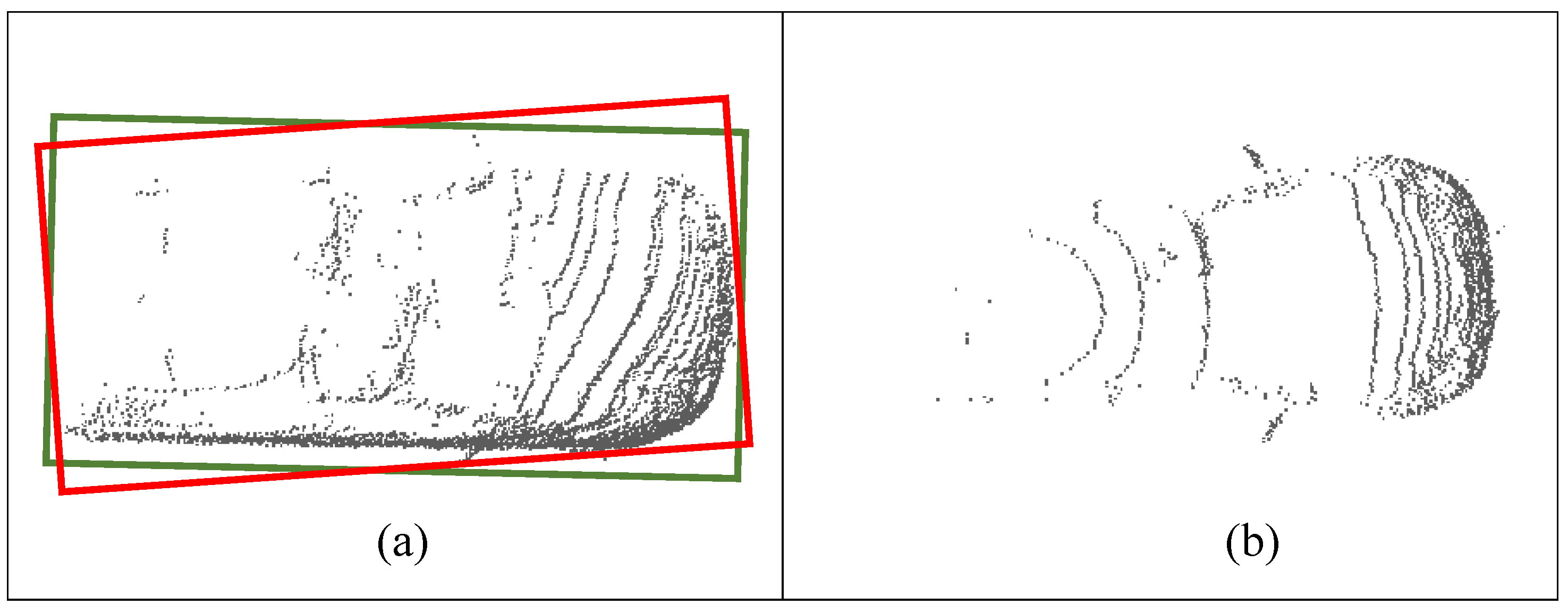
Model-based vehicle pose estimation methods [6,7,12,13] typically use rectangles or cuboids to represent vehicles, and then employ optimization or sampling techniques to generate the most probable pose of the vehicle. As shown in Figure 1, the side-view mirror of (a) causes a skew when estimating the orientation of the vehicle, where the orange rectangle is the predicted bounding box with model-based methods and the red rectangle denotes the ground truth.

Feature-based vehicle pose estimation methods typically rely on edge features and line fitting algorithms, such as L-shape fitting or Principal Component Analysis (PCA).

However, these methods rely heavily on the features of the side edge. When the side-edge is displayed incompletely, they struggle to accurately regress the orientation. As shown in Figure 1, the boundaries of the side-edge in target (b) are unclear, and measurements are approximately symmetrical about a certain ray of LIDAR. Hence, a single treatment for all measurements could encounter ambiguities if the estimated targets are of various shapes. In addition, it is crucial to ensure the limits of real-time performance for vehicle pose estimation, which can help save time for highly computational tasks such as tracking and path planning.

We present a novel solution, named the Pose Estimation Algorithm with Heuristic L-Shape Fitting and grid-based Particle Filter (PE-HL-PF), to address the challenges encountered in vehicle pose estimation in real-world traffic scenarios. PE-HL-PF leverages the divide-and-conquer approach to classify the shape of targets into symmetrical-like and asymmetrical-like types. For targets that are symmetrical to a LIDAR ray from the ego-car, we regress the orientation using a structure-aware weighted sum of the grid-wise velocity, which is achieved using the verified particle filter algorithm. Otherwise, asymmetrical-like ones are processed with the contour-based heuristic L-shape fitting method (HL). It extracts length-aware contours with visible constraints. Furthermore, it then selects the dominant contours and fit orientation with RANSAC. The proposed approach tackles the challenge of incomplete edge features that can lead to ambiguity in existing methods while also ensuring real-time performance, which is essential for computational tasks such as tracking and path planning. Our source code can be found at https://github.com/sunjingnjupt/PE-HL-PF (accessed on 27 February 2023).

We summarize our contributions as follows.

(1)

We propose a novel pose estimation method in this paper that combines heuristic L-shape fitting and grid-based particle filter techniques for the first time.

(2)

For symmetrical clusters, the target’ heading is derived by applying a structure-aware weighted average of grid-wise velocities. This manner improves the stability of pose estimation for sparse measurements.

(3)

For asymmetrical targets, we propose a contour-based heuristic L-Shape fitting module, which heuristically learns the length-aware contours and heading of the target. It enhances the model’s robustness to outliers while reducing its running time.

(4)

We conduct extensive experiments on the KITTI dataset to assess the performance of our PE-HL-PF model. Our PE-HL-PF model outperforms existing methods in terms of both runtime speed (10-fold increase) and accuracy (51% reduction in orientation estimation error and 27% decrease in position estimation error).

2. Related Works

In autonomous driving systems, both the ego vehicle pose estimation and the pose estimation of surrounding dynamic vehicles are important components of the perception system, and they interact with each other. In this section, we will first introduce the relevant work on ego vehicle pose estimation. Furthermore, we then review the dynamic vehicle pose estimation methods in termsof deep-learning-based vehicle pose estimation methods and traditional machine-learning-based vehicle pose estimation methods.

2.1. Ego Vehicle Pose Estimation Methods

In the field of vehicle pose estimation, determining the ego vehicle pose is of utmost importance. To achieve this, numerous scholars [14,15,16,17,18] have resorted to integrating various systems, such as the Global Navigation Satellite System (GNSS), cameras, and Inertial Measurement Unit (IMU) systems.

In [14], the authors proposed an integrated localization system that combines the GNSS, IMU, and wheel speed sensor (WSS). By using the Kalman filter to integrate various information, the localization accuracy is greatly improved. Ref. [15] utilizes the IMU and automotive onboard sensors to estimate the yaw misalignment. Thus, the measurement deviation of the IMU can be reduced, and the accuracy of state estimation can be improved. Ref. [16] fuses the information from the GNSS and an IMU and proposes a new vehicle slip angle (VSA) estimation method. Ref. [17] proposes a sideslip angle estimation that incorporates a dynamic model and visual information while considering acceleration error and camera measurement error. In ref. [18], authors proposed an algorithm for estimating the sideslip angle of an autonomous vehicle, which uses consensus and vehicle kinematics and dynamics synthesis. All the above methods have improved the estimated accuracy of ego vehicle pose estimation.

2.2. Deep-Learning-Based Vehicle Pose Estimation Methods

Recently, many famous deep-learning-based vehicle pose estimation methods have been proposed, which can be assigned to LIDAR-based methods or fusion-based methods.

Lots of LIDAR-based vehicle pose estimation methods have been proposed. PointPillars [19] converts the raw point data into a stacked pillar tensor and a pillar index tensor, then the features that can be learned from the pillars are put into a convolutional neural network (CNN), and the features from the last step are used by the detection head to predict 3D bounding boxes for objects. In order to reduce the computational cost, ref. [4] proposes a task-oriented and instance-aware down-sampling strategy to sample the interesting foreground points and perform the task of object detection. Similarly, Chen et al. [20] also designed a semantic-guided point sampling algorithm to help retain more useful foreground points. PillarNet [19] can reduce noise in depth estimation tasks by discarding redundant voxels and mapping sparse voxels back to the image space. It can effectively suppress noise and improve accuracy. Furthermore, VoxelNeXt [21] is a 3D object detection and tracking method that directly predicts objects based on sparse voxel features without relying on hand-crafted proxies. BTCDet [22] predicts the probability of occupancy in these regions. Therefore, with the learned occlusion information, the detection model can generate high-quality 3D proposals and refine the final bounding box.

Besides the LIDAR-based methods, other researchers aim to fuse the RGB data and the 3D point cloud data to improve the detector’s performance. Wang et al. [23] proposed sliding Frustums to aggregate local point-wise features for the task of 3D object detection. Liang et al. [24] designed a learnable architecture that mainly includes two streams: one for extracting image features, and another for extracting features from LIDAR Bird’s Eye View (BEV). They then designed the continuous fusion layers to bridge multiple intermediate layers on both streams. The detection header was used to generate the final detection results in BEV space. Yang et al. [25] proposed a map-aware detector to detect 3D point cloud objects. They exploited information on the road layout from the High-Definition (HD) maps and rasterized it onto the BEV, and then they connected the road mask representation with the LIDAR representation to produce the input representation. After that, they adopted a Fully Convolutional Network (FCN) to detect the point cloud objects. In order to handle the inferior image conditions, Bai et al. [26] proposed a soft-association mechanism with the famous transformer technology to fuse the LIDAR point and image pixel, which can adaptively fuse the object queries with useful image features. DeepFusion [27] designs the inverseAug and learnableAlign to align the transformed features from the LIDAR and camera data. InverseAug projects the key points obtained after the data augmentation via inversing geometric-related augmentations and fuses the LIDAR and camera data. Meanwhile, learnableAlign leverages cross-attention to dynamically capture the correlations between the image and LIDAR feature during fusion.

In general, deep-learning-based methods do well in vehicle detection with sufficient labeled point cloud data. As we all know, the precision of the deep-learning-based methods depends heavily on the training dataset [28]. However, it is hard to provide a wealth of training data sets for all kinds of scenarios with various complex obstacles in the actual scene, which is a main limitation for the wide applications of deep-learning-based methods. Another critical issue that exists in deep-learning-based methods is the high computational complexity. Highly computational resources are needed to meet the real-time constraint, limiting the broader application in the real world.

2.3. Traditional Machine-Learning-Based Vehicle Pose Estimation Methods

Traditional machine-learning-based methods can extract usable information about the object, such as trajectory and orientation, without considerable labeled training data. Due to their ease of deployment on the vehicle side, they have received increasing attention from industry and academia. These methods can be grouped into two separate directions: the first one is the model-based method, and the other one is the feature-based method.

2.3.1. Model-Based Methods

Model-based methods typically parameterize the rectangle of point cloud objects, and the most likely vehicle pose is determined through model iteration. Ref. [6] employs a likelihood field model to construct rectangles representing the vehicles, followed by using the Scaling Series algorithm to sample the estimated pose. On the other hand, Ding et al. [29] proposed an efficient convex hull-based pose estimation model that uses the minimum occlusion area as the criterion for deciding the best orientation.

The convex-hull-based methods usually calculate the 2D convex hull of the top-view projection of the objects. They then derive the 2D bounding boxes directly from the convex hull with various strategies, such as the minimum distance-based strategy [30] and the minimum area-based strategy [29]. The prior strategy chooses the optimal bounding box by minimizing the average distance between the points of the convex hull and the fitted rectangle with the convex hull edges. The other strategy selects the optimal bounding box by minimizing the area of the rectangle fitted with the convex hull edges. He et al. [31] presented a 3D pose estimation model based on the heuristic rules. It considers both the edge length and edge visibility to filter the convex hull-based orientations, and the tracking results are also used to smooth the orientation estimates. Benjiamin Naujoks et al. [13] proposed an orientation-corrected bounding box fitting method that uses rotating calipers to construct the minimum area rectangle of a convex hull. Then it fits the orientation of the rectangle with a heuristic search approach, and the computational time is significantly reduced. Liu et al. [32] used the convex-hull model to acquire a rectangle of the vehicular point clouds and then inferred the center position and the visible sides of the object rectangle, and they estimated the pose with the bounding box and position inference. In addition, ref. [33] proposes a novel orientation normalization vehicle modeling method containing an orientation normalization bounding box fitting model and a view-dependent orientation normalization model.

While model-based methods have achieved encouraging results in vehicle pose estimation, they are prone to being highly sensitive to noise and outliers in the data. Additionally, overfitting of the convex hull can lead to inaccurate or unstable results. For instance, side view mirrors can significantly influence the convex hull of a vehicle, especially when they extend beyond the main body. Therefore, there is a need for more accurate pose estimation models that can account for these issues and provide reliable and robust results.

2.3.2. Feature-Based Methods

The other common type of pose estimation approach is the feature-based method [34,35,36], they rely on the edge features to deduce the pose of the objects. The most famous type among the feature-based methods is the method based on the L-shape fitting. [34] partitions a cluster into two disjoint sets optimally using the least square error and then fits them with two perpendicular lines. Zhang et al. [35] proposed an efficient search-based L-shape fitting method to produce the bounding box of the vehicle detection. Firstly, they iterated through all the possible directions of the rectangle; for each rectangle oriented in that direction, they calculated the distance of all points to the rectangle’s edges as the corresponding square errors. They can find the optimal direction with the least squared error and fit the rectangle based on this direction. This method reaches a state-of-the-art performance in pose estimation. The method in [9] innovatively decomposes the L-shape fitting problems into two steps: L-shape vertex searching and L-shape corner point locating with 2D laser data, which can significantly reduce the computational complexity. Darms et al. [36] extracted the edge feature of the target from the raw data and estimated the target as a box, which is used in the tracking process. The aforementioned research has shown that these methods perform effectively when using laser data. With the development of the LIDAR, some researchers applied the feature-based method to fit the 3D point cloud objects.

Himmelsbach et al. [37] proposed a method that fits the dominant line of the point cloud segments in the $xy$-plane with random sampling consistency detection (RANSAC) to determine the orientation of the vehicle. In [38], a corner-edge-based algorithm is designed to fit the pose of the vehicle. It first finds the nearest corner of the target and uses the RANSAC to fit the L-shape-based orientations. The LIDAR-based 3D object perception method proposed in [39] compresses the 3D LIDAR data into a 2.5D occupancy grid and fits the bounding box of the point cloud objects by finding connected components of grid cells. Lalonde et al. [40] used covariance analysis to capture the spatial distribution of points and derived the orientation of the point cloud object with principal components analysis.

In order to improve the efficiency of the model, Ye et al. [41] extracted the points on the border and used an L-shape algorithm to fit these points into a polyline. Finally, it selects the longest line of polylines as the orientation of the cluster with the multi-layer laser. A fast RANSAC-based approach [8] maps the 3D points into the 2D grids and selects the boundary cells of the targets, then selects the visible cells and fits every possible orientation line with the selected cells by the RANSAC. Finally, it validates the best orientation from the all-fitted oriented lines.

When most feature-based methods deal with targets with specific geometric shapes, such as an L-shape, they have certain effectiveness. However, the performances become unsatisfactory when dealing with complex real-world traffic scenes that involve various shapes of point cloud targets. For instance, the L-shape-based methods [38,41] are limited to L-shaped targets and may not perform well with targets of other shapes, such as symmetrical ones. Besides, the L-shape-based methods [38,41] are also sensitive to noise and outliers when fitting the orientation.

Both model-based and feature-based methods for vehicle pose estimation have demonstrated promising results in certain scenarios. However, they may not be able to handle point cloud targets of various shapes simultaneously, which can lead to overfitting or underfitting of the models and result in inaccurate or unstable results. Moreover, most methods are susceptible to the presence of noise and outliers in the data, which can affect the accuracy and consistency of the results. Meanwhile, they are computationally expensive, especially for large datasets, and may require tuning of various parameters to obtain optimal results. To address these limitations, there is an urgent need for a robust and efficient pose estimation method that can handle point cloud targets of various shapes simultaneously, is resistant to noise and outliers, and has a reduced computational burden.

3. A Pose Estimation Algorithm with Heuristic L-Shape Fitting and Grid-Based Particle Filter (PE-HL-PF)

Given a point cloud cluster $P=\left\{p_1,p_2,\dots ,p_i,\dots ,p_N\right\}$ where N denotes the number of the cluster, and the ${\mathit{p}}_{\mathit{i}}$ = ${\left(x_i,y_i,z_i\right)}^T$ denotes the Euclidean coordinate with regard to the ego-coordinate system, we will firstly fit a bounding box to estimate the vehicle pose in $xy$-plane. Afterward, we use the z value of the points to fit a 3D bounding box for the object. The overall diagram of the proposed Pose Estimation algorithm with Heuristic L-shape fitting and a grid-based particle filter (PE-HL-PF) are shown in Figure 2. Adopting the thought of divide and conquer, PE-HL-PF introduces a geometric shape classifier to divide clusters into symmetrical-like or asymmetrical-like ones for the first time. Furthermore, for asymmetrical-like ones, a contour-based heuristic L-shape fitting method (HL) is introduced. It extracts the length-aware contours and regresses orientation with dominant contours. Furthermore, the symmetrical clusters regressed the orientations with a verified particle filter algorithm (PF). The details about our PE-HL-PF are given in the following subsections.

3.1. Geometric Shape Classifier & Symmetrical Estimation Model for Vehicles

In real-world autonomous driving scenes, there exist a number of point cloud clusters with various shapes. Such as clusters in Figure 2, the symmetrical point cloud clusters that are labeled with orange ellipses, are rightly symmetrical about a specific LIDAR ray from ego-car. Additionally, the L-shape clusters, which are marked with rectangles in Figure 2, are asymmetrical relative to the ego-car. Many of the currently available methods treat all measurements with a uniform approach, such as convex-hull-based or L-shape-based pose estimation methods, which may result in inaccuracies when attempting to estimate the pose of clusters with varying shapes. To alleviate this, we introduce the Geometric Shape Classifier (GSC) to categorize clusters as either symmetrical or asymmetrical. Subsequently, we develop separate modules for estimating symmetrical and asymmetrical poses to process these clusters.

3.1.1. Geometric Shape Classifier

Clusters are categorized as symmetrical if they meet two criteria: the calculated width falls within a predefined threshold and the number of symmetrical contours exceeds a specified threshold. It should be noted that the symmetrical designation refers to approximate symmetry rather than strict symmetry and is employed for the purpose of point cloud processing by type. Figure 3 provides an illustration of the Geometric Shape Classifier. Further details regarding the Geometric Shape Classifier and symmetrical pose estimation model are provided in this subsection.

To calculate the width of the cluster in the first criteria, we define two endpoints $p_{max}$ and $p_{min}$ in a cluster according to the observation azimuths described with Equation (1).

$${\theta }_{obz}\left(p_i\right)=atan2\left(y_i,x_i\right)$$

(1)

We define $p_{max}$ and $p_{min}$ as the points that produce the maximum observation azimuth ${\theta }_{obz}\left(p_{max}\right)$ and the minimum observation azimuth ${\theta }_{obz}\left(p_{min}\right)$ on the target, respectively. Besides, the angle covered by the point cloud cluster is defined as $\Delta {\theta }_{vehicle}={\theta }_{obz}\left(p_{min}\right)-{\theta }_{obz}\left(p_{max}\right)$. As shown in Figure 3a, the $\frac{1}{2}$ width of the cluster is obtained by selecting the longer distance between the endpoints and the angle bisector $l_b$ of $\Delta {\theta }_{vehicle}$. If the width of the cluster falls within the predefined range $\left[widt{h}_s,widt{h}_l\right]$, we proceed to the second step of selecting symmetrical clusters by calculating the number of symmetrical contours, as demonstrated in Figure 3b.

To extract the contours of cluster P, the GSC algorithm divides P into a set of segments $S_{Symmetric}=\left\{s_1,s_2,s_3,\dots ,s_j,\dots ,s_M\right\}$ evenly, where M represents the number of segments. The contour is then obtained by selecting the point in each segment that has the smallest distance to the origin point. Once the contours have been extracted, their distances are compared with determine if the cluster is symmetrical about the $l_b$. For instance, we compare the distance values of the contour points in $s_j\left(i=1,2,\dots ,M\right)$ and $s_{M-j+1}\left(j=1,2,\dots ,M\right)$ separately. If the distance difference between the corresponding contour points is less than the predefined threshold $D_{sym}$ we will define the two contours as symmetrical. If the number of symmetrical contours on the cluster exceeds a specified threshold $N_{sym}$, we will define the cluster as symmetrical.

3.1.2. Symmetrical Estimation Model

For the symmetrical clusters, the LIDAR measurements are modeled as a dynamic occupancy grid with particles, as proposed in [42]. Specifically, the point cloud scene is represented by 2-D discrete grids, and the vehicles are represented by a set of particles $T=\left\{t_i\left|t_i=\left(x_i,y_i,v_{xi},v_{yi},a_i\right),i=1,\dots ,N_T\right.\right\}$, where $x_i$ and $y_i$ denote the position of particle $t_i$ along $x$-axis and $y$-axis, $v_{xi}$,$v_{yi}$ denotes the velocity along $x$-axis and $y$-axis, $a_i$ denotes the age of the particle existence, and the $N_T$ denotes the number of particles. By utilizing the coordinate mapping function $f\left(·\right)$, the particle’s position and velocity on the occupancy grid can be denoted as $T=\left\{t_i\left|t_i=\left(c_i,r_i,v_{ri},v_{ci},a_i\right),i=1,\dots ,N_T\right.\right\}$. The dynamic occupancy grid map can be represented as a binary grid, where grids occupied by particles are assigned a value of 1, while unoccupied grids are set to 0.

Subsequently, the particles are transferred from the previous frame $t-1$ to the current frame t, utilizing the estimated velocity and motion parameters of the ego vehicle. As a result, the set ${\widehat{O}}_G$ can be used to represent the index of predicted occupied grids in the current frame. In addition, the index of measured occupied cells of the vehicles on the current frame can be represented as ${\overline{O}}_G$. The particles within overlapping grids in $O_G$ are resampled, while those in non-overlapping cells are destroyed. The overlapping map can be represented with Equation (2):

$$O_G={\widehat{O}}_G\cap {\overline{O}}_G$$

(2)

Upon completion of a cycle of estimation for each particle, the velocity of each grid can be estimated as the average velocity of the particles whose position coincides with the position of the grid. The grid-wise velocity can be computed with Equation (3). Where $v_{c_g}and{v}_{r_g}$ denote the velocity of the grid along column and row, and $(r_g,c_g)$ represents the index for the grid along row and column.

$$\left(v_{c_g},v_{r_g}\right)=\frac{{\displaystyle \sum _{t_i\in T,f\left(x_i\right)=r_g,f\left(y_i\right)=c_g}}\left(v_{c_i},v_{r_i}\right)}{\left|\left\{t_i\in T\left|r_i=r_g,c_i=c_g\right.\right\}\right|}$$

(3)

Next, the velocity of the vehicles is computed using a structure-aware weighted average of velocities for the corresponding grid. Specifically, greater weight is assigned to the velocity of contour grids relative to that of inner grids, based on statistical findings indicating that the speed predicted by the edge grid more closely approximates the true value. Furthermore, we apply the direction of the velocity as the estimated heading of symmetrical clusters. Lastly, the oriented bounding box of symmetrical clusters is fitted, referring to the work in [13].

3.2. Asymmetrical Pose Estimation Model for Vehicle

Asymmetrical clusters are typically characterized by the following geometric features in contrast to symmetrical clusters. (a) Asymmetrical clusters usually have two visible sides with different lengths, whereas symmetrical clusters have one or two sides with symmetrical lengths. (b) On the side view of asymmetrical clusters, there are many irregularly raised points, such as a side view mirror on the side surface, making it difficult to use all contours fitting orientation with traditional L-shaped-based methods directly.

Regarding characteristic (a), the asymmetrical model extracts contours based on the visible sides’ length. Specifically, it divides the clusters into multiple segments with different coverage angles, where the coverage angles correspond to the length of the located sides. This approach allows for learning more geometric features around the longer sides.

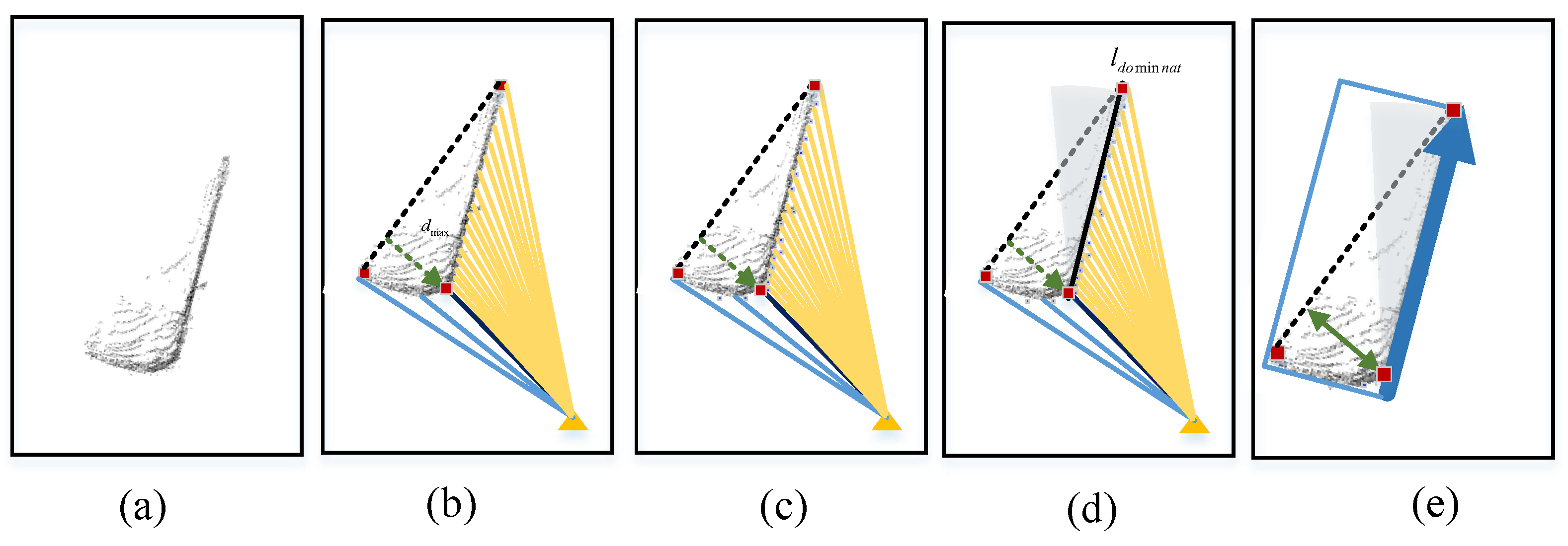
For the characteristic of (b), the asymmetrical model has conducted itself in the following two manners. Firstly, it directly selected the optimal contours around the rotated longer side instead of dealing with the L-shape fitting problem as a complex optimization problem. Secondly, the asymmetrical model fits the orientation line with RANdom SAmple Consensus (RANSAC) algorithm, which is robust when coping with irregular raised contours on the side-view. The illustration of the process for the asymmetrical model is shown in Figure 4. The details of the asymmetrical model are discussed in the following subsections, which contain two parts: length-aware contour extraction and orientation fitting with optimal contours.

3.2.1. Length-Aware Contours Extraction

As mentioned above, the asymmetrical clusters contain two visible sides with different lengths, and we extract contours according to the length of the visible sides. The first step is to find the corner point of the asymmetrical cluster and obtain two visible sides by connecting the line between the endpoints and the corner point. Specifically, the process of acquiring the corner point is shown as follows.

Firstly, as shown in Figure 4, we utilize $\mathit{l}$ to indicate the vector between endpoints ${\mathit{p}}_{max}$ and ${\mathit{p}}_{min}$, then, the foot point $foo{t}_{\mathit{l}}\left({\mathit{p}}_{\mathit{i}}\right)$ of ${\mathit{p}}_{\mathit{i}}$ corresponding to $\mathit{l}$ can be calculated through Equation (4)

$$foo{t}_{\mathit{l}}\left({\mathit{p}}_{\mathit{i}}\right)={\mathit{p}}_{\mathit{max}}-\frac{〈{\mathit{p}}_{\mathit{max}}-{\mathit{p}}_{\mathit{i}},\mathit{l}〉}{〈\mathit{l},\mathit{l}〉}·\mathit{l}$$

(4)

where $〈·〉$ denotes the inner product. Consequently, the relative distance $d\left({\mathit{p}}_{\mathit{i}},\mathit{l}\right)$ between point ${\mathit{p}}_{\mathit{i}}$ and vector $\mathit{l}$ is obtained using Equation (5)

$$d\left({\mathit{p}}_{\mathit{i}},\mathit{l}\right)=〈\tilde{\mathit{n}},{\mathit{p}}_{\mathit{i}}-{\mathit{p}}_{\mathit{max}}〉$$

(5)

where $\tilde{\mathit{n}}$ is the normal vector of $\mathit{l}$. We design two constraints for corner point $p_c$ extraction: The distance $d\left({\mathit{p}}_{\mathit{c}},\mathit{l}\right)$ should be the maximum among $\left\{d\left({\mathit{p}}_{\mathit{i}},\mathit{l}\right),i=1,2,\dots ,N\right\}$, where N is the number of points in the cluster.

To cope with the outliers and ensure the validity of the ${\mathit{p}}_{\mathit{c}}$, ${\mathit{p}}_{\mathit{c}}$ and the origin $O_e$ of ego-car coordinate system should be on the same side of $\mathit{l}$. The process of finding the corner point can be formulated using the following Equation (6).

$$\left\{\begin{array}{c}\underset{{\mathit{p}}_{\mathit{i}}\in P}{max}d\left({\mathit{p}}_{\mathit{i}},\mathit{l}\right)\hfill \\ s.t.d\left({\mathit{p}}_{\mathit{i}},\mathit{l}\right)·d\left(O_e,\mathit{l}\right)>0\hfill \end{array}\right.$$

(6)

Having found the corner point ${\mathit{p}}_{\mathit{c}}$, we connect the corner point ${\mathit{p}}_{\mathit{c}}$ and ${\mathit{p}}_{\mathit{max}}$ with the ${\mathit{l}}_{\mathit{max}}$, and connect the ${\mathit{p}}_{\mathit{min}}$ and ${\mathit{p}}_{\mathit{c}}$ with ${\mathit{l}}_{\mathit{min}}$.

Contours are obtained in different sector segments with different angular resolutions around the longer side and shorter side, based on the lengths of ${\mathit{l}}_{max}$ and ${\mathit{l}}_{min}$. Specifically, the contour point is the point nearest to the ego-car among all points within a segment.

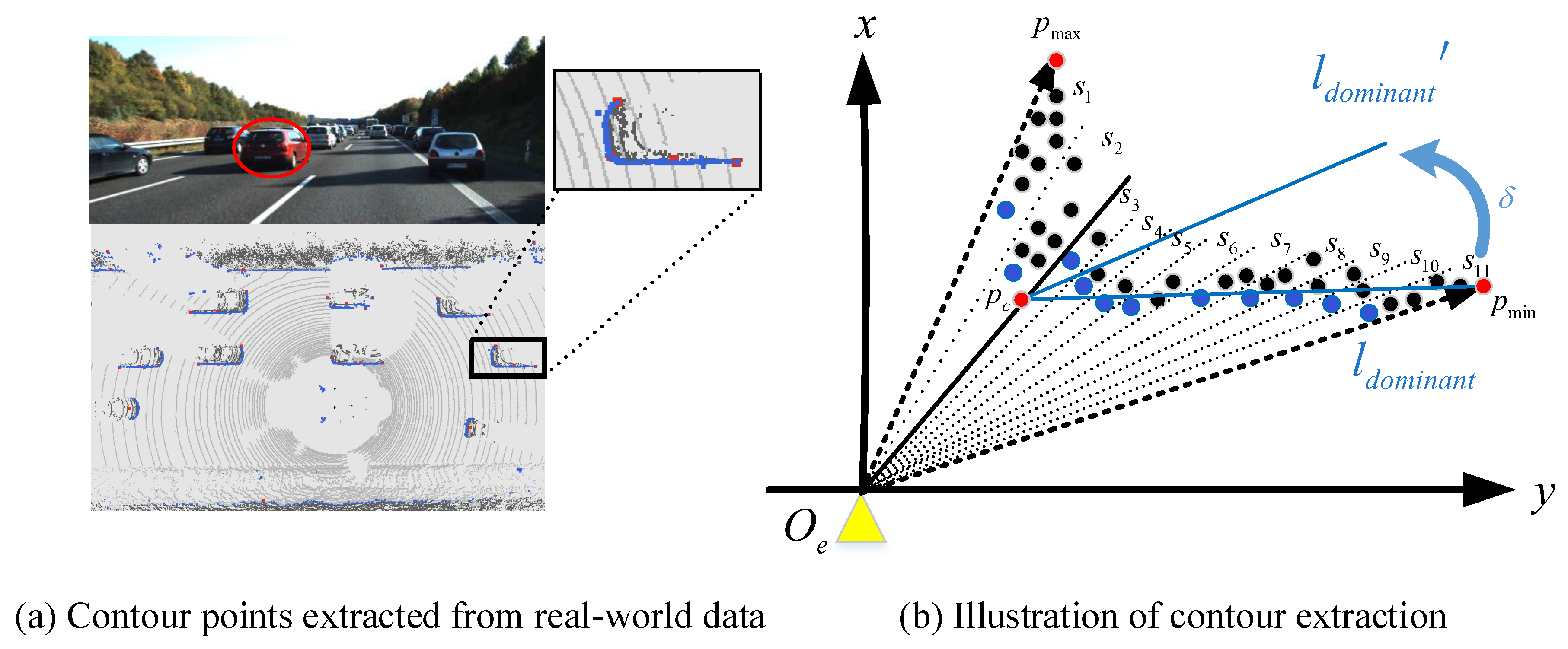
3.2.2. Orientation Fitting with the Optimal Contours

In general, the orientation line of a vehicle is often parallel to its longest side. According to this common sense, we heuristically choose the contours around the longer side of the edges to fit the orientation of the target. Nevertheless, apart from that, there are lots of contours that stay away from the outline, such as the contour point in segment $s_3$ in Figure 5, which may result in skewing of predicted orientation lines. We overcome this issue by selecting optimal contours in a range that excludes unqualified contours.

Specifically speaking, we use the longer edge ${\mathit{l}}_{max}$ as the dominant line ${\mathit{l}}_{dominant}$. Furthermore, the rotated dominant ${{\mathit{l}}_{dominant}}^{\prime }$ can be achieved by rotating ${\mathit{l}}_{dominant}$ around $p_c$ from the direction of ${\mathit{l}}_{dominant}$ to the direction away from the ego-car with the angle $\delta$, as shown in Figure 5b. The slope value ${k_{dominnat}}^{\prime }$ of ${{\mathit{l}}_{dominant}}^{\prime }$ can be calculated with Equation (7)

$${k_{dominnat}}^{\prime }=tan\left({\theta }_l+\delta \right)=\frac{tan\left({\theta }_l\right)+tan\delta }{1-tan\left({\theta }_l\right)tan\delta }$$

(7)

where ${\theta }_l$ represents the slope observation angle of ${\mathit{l}}_{dominant}$. The optimal contours $c_j^{*}$ can be obtained with the following constraint:

$$d\left({\mathit{c}}_{\mathit{j}}^{*},{{\mathit{l}}_{dominant}}^{\prime }\right)·d\left({\mathit{p}}_{\mathit{dominant}},{{\mathit{l}}_{dominant}}^{\prime }\right)>0$$

(8)

where ${\mathit{p}}_{\mathit{dominant}}$ denotes the other endpoint of the ${\mathit{l}}_{dominant}$ except ${\mathit{p}}_{\mathit{c}}$.

Figure 5 shows the schematic illustration for optimal contours extraction. As we can see, the points around the shorter edge ${\mathit{l}}_{min}$ are divided into two segments $\left\{s_1,s_2\right\}$, and the points around the longer edge ${\mathit{l}}_{max}$ are divided into nine segments $\left\{s_3,s_4,s_5,\dots ,s_{11}\right\}$. We select the contour points in each segment, which are marked with blue.

The RANSAC [8] algorithm is used to fit the orientation line $l_v$ of the vehicle because it is robust to outliers and has a lower computational load. After obtaining the yaw angle of orientation, the position of the target is inferred according to the method in [13]. The obtained tight bounding box is shown as the black rectangles in Figure 4. To handle occlusions, such as objects in front of or behind the ego-car, the width and length of the estimated bounding box are inferred by setting a predefined length.

Since the above processes are based on the $XY-$ plane, In order to acquire the height of the estimated bounding box, we use the following Equation (9)

$$h=z_{max}-z_{min}$$

(9)

where $z_{max}$ denotes the maximum value in the $z-$ dimension of the original $XYZ$ coordinate system. Similarly, $z_{min}$ indicates the minimum value of the $z-$ dimension of the original $XYZ$ coordinate system.

4. Experimental Results and Analysis

The details of the dataset and evaluation metrics are given in Section 4.1, we also give the implementation details and compare methods in Section 4.2. Then we report and analyze the experimental results with aspects of estimated results (angle error and position error) and running time. The example video can be found online (https://youtu.be/FMX1Pya6qwg (accessed on 27 February 2023)).

4.1. Dataset and Evaluate Metrics

To evaluate the performance of our proposed method, PE-HL-PF, we conducted experiments using the KITTI object tracking evaluation dataset [43], which consists of 21 training sequences and 29 test sequences. Similar to [12], we selected the most common category, “car”, to evaluate our performance.

As the ground truth of the test sequences was unavailable, we utilized the training sequences for training and evaluating our methods. Specifically, following the standard protocol as outlined in [23], we partitioned the training data into two subsets in a 1:1.1 ratio. Specifically, one subset was utilized for adjusting the model’s parameters, while the other was used for evaluating its performance. The evaluation subset consisted of sub-dataset IDs 0000, 0002, 0006, 0007, 0008, 0009, 0010, 0013, 0019, and 0020. The selected sub-datasets comprise a wide range of complex scenarios, including highways, cities, and suburban areas. And the measurements exhibit various shapes due to different measurement views and mutual occlusion between objects in these datasets. Further details about the selected sub-datasets are provided in

Table 1. Detail of the selected sub-datasets.

ID of Sub-Dataset	Number of Frames	Number of Dynamic Objects
0000	153	535
0002	232	1142
0006	269	661
0007	799	2488
0008	389	1339
0009	803	3135
0010	293	673
0013	339	124
0019	1059	1413
0020	837	6259
Total	5173	17,769

.

We employed widely used evaluation metrics, including position error and angle error, to evaluate the accuracy of PE-HL-PF. Furthermore, the running time was also measured to verify that our PE-HL-PF is computationally efficient.

Position error is defined as the Euclidean distance between the center of the ground truth bounding box and the center of the estimated bounding box. And the ground truth is provided by the KITTI website. In light of the fact that the estimation model aims to accurately estimate the location of the center of the predicted bounding box, it is clear that a good estimate is reflected by a small position error.

Angle error refers to the deviation between the ground truth and the estimated orientation. PE-HL-PF pursues the precisely oriented bounding boxes for the surrounding clusters since a precise predicted orientation is crucial to downstream tasks such as tacking. Thus, a good estimated model has a small angle error.

4.2. Implementation Details and Compared Methods

We use a standard office computer with a 2.60 GHz Intel Core i5 CPU and 7.5 Gb of RAM. Our approach and comparison methods are implemented in the C++ framework on the Ubuntu system. In order to facilitate the visualization of the algorithm’s performance, we adopted the GUI library Qt5, open-source OpenGL library, and the QGLViewer library. Furthermore, we also added numerous interactive buttons to facilitate the parameter adjustment. Furthermore, there is no parallelization enabled.

In this paper, the segmentation and ground plane line extraction algorithm proposed in [11] is applied to remove the ground points, and residual obstacle points are clustered into many clusters with a seed-filling connected components labeling algorithm [44]. Moreover, we search a wide range of the following values and select those that yield the best estimation.

During learning the optimal parameters, we considered various optimization algorithms, such as the genetic algorithm [3], grid search method, etc. As in ref. [45], we determined the predefined values of each parameter based on the statistics of the training dataset. Subsequently, we performed an iterative optimization of individual parameters to achieve the best results. Specifically, the wide range for width threshold is $\left[widt{h}_s,widt{h}_l\right]$, which is determined as [1–2, 2–3] m, and we find the best value of the range to be [1.3, 2.3] meters. The value of $N_{sym}$ is in the range of 10, 20, 30, and 40, and we set it at 20. For compared segment groups, the threshold values $D_{sym}$ are set in the range of [0, 0.5]. Besides, the threshold value of the symmetrical segment number $N_{sym}$ is in the range of [5, 20]. The value of $\delta$ is in the range of [1, 60] degrees.

To verify the effectiveness of the PE-HL-PF algorithm, we compare its estimation performance with state-of-the-art vehicle pose estimation methods such as PE-CPD [12], PE-CHM [32]. PE-CPD [12] proposes a vehicle detection model that uses coherent point drift. It consists of two parts: a dynamic vehicle detection component with an adaptive threshold, and a dynamic vehicle confirmation component that employs the scaling series algorithm. PE-CHM [32] fits the point cloud object into a polygon with the convex-hull algorithm based on the minimum distance and finds the pose of the vehicle with a fixed side model. We compare our estimated angle error and location error with the above methods. Furthermore, we also evaluate the components of our PE-HL-PF with different settings.

4.3. Experimental Results

In this subsection, we evaluate the performance of the proposed PE-HL-PF with the compared vehicle pose estimation methods in terms of estimated orientation error, position error, and running time. Furthermore, we design ablation studies to verify the effectiveness of different components.

4.3.1. Estimated Performance of PE-HL-PF

As for the evaluation of pose estimation, we first show the estimated results of orientation and position errors. We show the angle errors (degree) for ten selected datasets in

Table 2. Comparison of the mean orientation errors with ground truth object (deg).

ID of Sub-Dataset	PE-CPD	PE-CHM	PE-HL-PF
0000	3.87	4.75	1.83
0002	4.31	4.04	2.87
0006	4.01	3.65	2.49
0007	5.32	4.97	2.85
0008	5.21	4.03	3.42
0009	4.59	3.69	3.59
0010	4.83	3.87	2.88
0013	4.62	4.47	1.82
0019	3.97	4.02	3.10
0020	4.51	4.31	2.89
Average	4.52	4.18	2.77

. In addition to angle errors, we also compare the estimated position error (meter) of our PE-HL-PF with that of the state-of-the-art methods in

Table 3. Comparison of the mean position errors with ground truth object (meter).

ID of Sub-Dataset	PE-CHM	PE-CPD	PE-HL-PF
0000	0.63	0.55	0.25
0002	0.70	0.61	0.42
0006	0.43	0.52	0.37
0007	0.54	0.63	0.36
0008	0.56	0.47	0.51
0009	0.59	0.55	0.52
0010	0.55	0.51	0.40
0013	0.51	0.42	0.30
0019	0.43	0.44	0.32
0020	0.40	0.50	0.34
Average	0.53	0.52	0.38

.

As shown in Table 2, the performance of orientation estimation for PE-CHM [32] is not as good as that of our PE-HL-PF method. The results indicate that the orientation error estimated by PE-HL-PF is 1.41 degrees lower than that of PE-CHM. PE-CHM requires polygon fitting before orientation fitting and iterates over all polygon edges to fit the orientation. However, this approach can lead to the over-fitting of convex hulls due to irregular objects on the vehicle surface, such as mirrors, resulting in inaccurate orientation estimation. In contrast, our PE-HL-PF method uses RANSAC to fit the orientation using optimal length-aware contours, ensuring that the fitting of the orientation is not affected by the irregular object. In this manner, our method reaches a robust performance in the orientation fitting when dealing with the asymmetrical measurements.

Additionally, we also compare the PE-HL-PF with the PE-CPD [12], which involves knowledge of motion coherence. By comparing the mean of the orientation error in 10 selected sequences, we find that our method improves by 1.75 degrees. Figure 6 illustrates the distribution of orientation error among the state-of-the-art pose estimation methods in dataset 19. As shown in Figure 6a, most results for objects are distributed from 0 to 3 degrees with PE-HL-PF. Conversely, there is a higher proportion of results between 3 and 20 degrees for PE-CPD and PE-CHM. These findings suggest that the performance of PE-HL-PF is more consistent and stable when compared with the other methods.

Except for angle errors, we also evaluate our methods with a center location error, which evaluates the accuracy of the estimated bounding box. The performance of our proposed PE-HL-PF method is compared with PE-CHM and PE-CPD in Table 2. The results indicate an improvement of at least 0.14 m (0.52-0.38) compared with the other methods. That is due to the fact that our PE-HL-PF derives position from the estimated orientation, and the combination of the L-shape fitting module and grid-based particle filter fitting module significantly improves the orientation estimation performance on point clouds with diverse shapes.

Besides, Figure 7 shows the position error distribution of the PE-HL-PF, PE-CPD, and PE-CHM. It can be observed that the position errors of most objects are less than 0.15 m. Based on the aforementioned observations, it is evident that our proposed PE-HL-PF method is more precise and stable in vehicle pose estimation when compared with PE-CPD and PE-CHM.

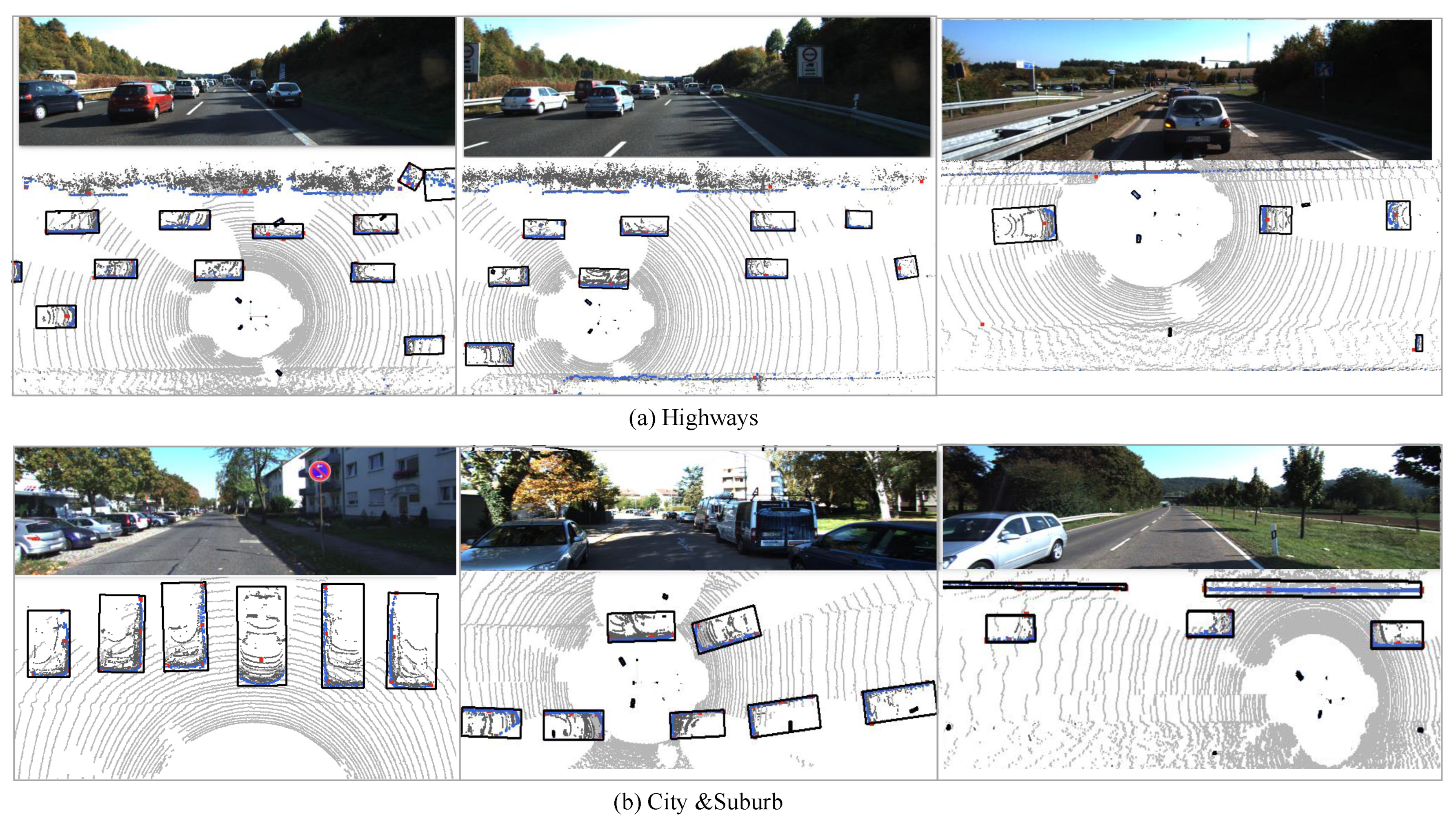
Qualitative results of PE-HL-PF are shown in Figure 8. It contains six roadway scenarios in the KITTI Vision Benchmark Suite. As for Figure 8, the upper three scenarios are on the highways, and the lower parts are the scenarios of the city and suburb. In addition, each scenario consists of an RGB image and a LIDAR point cloud image, where the black rectangles are the fitted bounding boxes of the objects. As shown in Figure 8, even for some difficult shapes of clusters, such as clusters with side-view mirrors or symmetrical-like clusters, an accurate estimation result can be achieved using our method. We can conclude that our method achieves an encouraging estimated performance in different scenarios.

4.3.2. Estimated Result of Different Components of PE-HL-PF

To analyze individual components of our proposed method, such as the geometric shape classifier and the asymmetrical and symmetrical pose estimation module, we also conduct ablation experiments to estimate the pose of vehicles without the three components. As the orientation error is directly influenced by the above components and the estimated orientation line determines the oriented bounding box, we apply angle error to estimate the effectiveness of the various components. All models are evaluated on the selected KITTI tracking datasets.

The results of mean angle errors with different individual components are shown in

Table 4. Mean angle error with different individual components of PE-HL-PF (deg).

	Classifier & Symmetrical Estimation Module	Asymmetrical Estimation Module		Angle Error
		Length-Aware Contours	Dominant Contours Extraction
1	✓	✓	✓	2.77
2		✓	✓	3.28
3	✓	✓		2.91
4	✓		✓	3.01

. Setting one verifies PE-HL-PF with all components, and setting two estimates the objects’ pose only with our asymmetrical estimation module. Upon comparing the results of setting one and setting two, it is evident that setting one yields a 0.51-degree improvement (3.28–2.77). This outcome could be attributed to the utilization of the particle filter algorithm in setting one, which employs the low-level velocity of grids to fit the orientation of the sparse symmetrical clusters. This manner is more robust than the shape of point cloud clusters.

Setting three extracts the visible length-aware contours and fits all possible perpendicular lines with RANSAC for the asymmetrical-like clusters. The processing manner for the symmetrical-like cluster is the same as setting one. By comparing setting one and setting three, we can find that the strategy of dominant contour extraction boosts a 0.14-degree improvement. That may be because the dominant contour extraction can cope with the outliers, such as points on the side-view mirror, thus improving the accuracy of the estimated orientation. In setting four, we extract contours with a regular angular resolution for asymmetrical-like clusters. The result of setting four illustrates that more detailed geometric feature extraction can assist the orientation fitting.

4.3.3. Running Time Comparison

Table 5. Comparison of the mean runtime for 100 objects (ms).

ID of Sub-Dataset	PE-CHM	PE-CPD	PE-HL-PF
0000	15.31	66.01	1.12
0002	15.2	64.98	1.11
0006	13.7	67.01	1.01
0007	9.85	65.32	0.97
0008	9.56	64.32	0.66
0009	13.56	63.80	0.93
0010	11.05	66.34	0.78
0013	14.21	66.21	1.31
0019	19.45	67.01	1.39
0020	16.03	65.31	1.22
Average	13.79	65.63	1.05

presents a comparison of the mean running time (in milliseconds) for 100 point cloud objects in various scenarios. PE-HL-PF has improved the running efficiency by dozens of times compared with existing models, such as PE-CHM and PE-CPD. This improvement is primarily due to the fact that our algorithm directly fits the orientation line using optimal dominant length-aware contours, as opposed to fitting all possible perpendicular lines to the object boundaries. This leads to a significant reduction in computational load.

Based on the data presented in Table 5, we can conclude that our PE-HL-PF algorithm is capable of estimating 100 objects in approximately 1 millisecond. In conclusion, the PE-HL-PF algorithm has demonstrated real-time performance in the estimation of the pose of point cloud objects in real-world scenarios.

5. Conclusions

This paper introduces a novel pose estimation algorithm, the PE-HL-PF, which employs heuristic L-shape fitting and a particle filter algorithm for bounding box fitting. To improve accuracy, a classification module is employed to distinguish between symmetrical and asymmetrical point cloud clusters. The algorithm includes separate modules for estimating the pose of symmetrical and asymmetrical clusters, taking advantage of the differential treatment of the two types. Additionally, the proposed method selects optimal contours around the longer edge to fit the vehicle’s orientation, thereby reducing computational complexity. The results show that the proposed method achieves high estimation performance compared with existing approaches.

The results of extensive experiments on the KITTI dataset have demonstrated the effectiveness of our proposed PE-HL-PF algorithm, enabling us to accurately generate an oriented bounding box for vehicle pose estimation while meeting real-time constraints. In our future work, we aim to further validate the effectiveness of our algorithm on additional datasets and explore its applicability to a broader range of scenarios.