Optimal Layout of Electric Vehicle Charging Station Locations Considering Dynamic Charging Demand

Abstract

This paper proposes an optimization method for electric vehicle charging station locations considering dynamic charging demand. Firstly, the driving characteristics and charging characteristics of the electric vehicle are obtained based on the driving trajectory of the electric vehicle, and the charging demand is predicted using a Monte Carlo simulation. Then a mathematical model with the goal of minimizing the overall cost is constructed, and the impact on carbon emissions is considered in the model. In order to better solve the location model, an improved whale optimization algorithm based on a hybrid strategy is proposed. Finally, the location problem of Shenzhen electric taxi charging stations is analyzed as an example. The results show that when the number of charging stations is set to 19, the comprehensive cost is the smallest and the energy saving and emission reduction effect is good. The improved whale optimization algorithm also has higher solution accuracy and convergence speed than other classical algorithms.

1. Introduction

Recently, the vigorous development of the automobile industry has also brought many problems to society, among which air pollution and energy consumption are the most prominent [1]. To reduce dependence on oil and other energy sources, road traffic becomes key [2,3]. At present, more and more people are choosing electric vehicles when buying vehicles [4,5]. Compared with traditional fuel vehicles, existing new energy vehicles can reduce carbon emissions by about 15 million tons per year. The electric vehicle industry has been further developed under the drive of a low-carbon economy and a new energy strategy. However, its travel reliability still needs to be improved [6,7].

Mileage anxiety has become a core concern for consumers. As the supporting facilities for new energy vehicles, charging piles are also in a rapid development stage. Before 2020, the advanced construction mode was adopted for the construction of charging stations. Although this mode can increase the number of charging piles rapidly, it is not a benign demand-driven construction mode. As of March 2022, the ratio of car piles in China was about 2.9:1. However, according to statistical data, in 2021 the average utilization rate of public charging piles in 22 cities in China was less than 10%. The main reason for the low service efficiency of public charging piles in big cities was uneven distribution.

At present, the cruising range of electric vehicles has increased, but it is still difficult to meet the needs of users. In particular, vehicles such as taxis and ride-hailing vehicles have a greater need for charging due to their long daily mileage [8,9]. Taxi travel is bound to have a close connection with the urban road network. The driving characteristics and charging behavior of taxis will be affected by passengers’ travel rules, urban road network structure, and the distribution of charging facilities [10,11]. Conversely, taxi drivers’ driving habits and vehicle battery life will also have a great impact on road traffic flow. Therefore, the establishment of an accurate charging demand model for electric vehicles will be beneficial to the prediction of charging load. It is also the premise of charging station site selection.

Previously, it was difficult to collect trajectory data on electric taxis. Therefore, some scholars used the trajectory of fuel vehicles to replace the trajectory of electric vehicles in research on charging demand forecasting [12,13,14]. Kontou et al. [14] studied the relationship between the coverage rate of public charging facilities and charging probability by using the trajectory data of oil-fired taxis. Due to the different types of vehicles, taxi drivers’ driving habits will change accordingly. Obviously, the results obtained by using the trajectory of fuel vehicles will not conform to the actual situation. With the continuous improvement of data, many scholars have also begun to use electric vehicle trajectory data for charging demand prediction and site selection planning [8,15,16,17].

To some extent, the charging demand forecasting model based on the trajectory data of electric vehicles describes the spatial and temporal distribution characteristics of the charging load. However, it only considers the load characteristics of electric vehicles and ignores the randomness of movement which is easily affected by traffic factors in the process of vehicle driving. To this end, Xu et al. [18] predicted the charging demand of charging stations by analyzing the dynamic driving process of vehicles. In the process of analysis, information such as traffic conditions and power grid status is also included in this study. Tang et al. [19] and Xing et al. [20] introduced the theory of the traffic travel chain into research on the charging demand predictions of electric vehicles.

The charging demand forecast is the basis for planning the location of charging stations. According to the spatiotemporal distribution characteristics of electric vehicle charging demand, it is possible to better discover charging hotspots and inappropriate sites. From the perspective of the facility location model, the classic facility location models include the median model [21], the central model, and the coverage model [22]. With the deepening of research, the extended location problem was developed from the classic location model. The extended location problem can be divided into many categories according to the different practical application problems, such as the asymptotic coverage model, the alternate coverage model, and the hierarchical location and competitive location model. The OD matrix is often used to describe the characteristics of vehicle travel distribution [23,24]. From the optimization goal, the location model is mainly divided into three categories. The first category is the model established from the user’s point of view, such as the model with the minimum charging cost of electric vehicles [25], the model with the highest charging satisfaction [26], etc. The second type is the model established from the perspective of the enterprise, such as the model with the smallest operating cost [27,28], and the model with the highest utilization rate of charging piles [29,30]. The third category is the model established by taking into account the interests of users and enterprises [31,32,33]. Further, according to the existing research, we can calculate the carbon dioxide emissions produced by this trip through the mileage of the vehicle [34,35,36,37]. This allows a better comparison of the environmental impact of using a gasoline vehicle versus using an electric vehicle.

The intelligent optimization algorithm is usually used to solve the location problem. The whale optimization algorithm (WOA) is a new intelligence optimization algorithm [38]. The WOA has the advantages of simple operation and fast convergence but also has the disadvantage of low solution accuracy, and it is easy to fall into local optimal solutions [31,39,40]. Zhang et al. [31] applied the WOA to the solution of the location model. After improving the WOA from many aspects, it was found that the convergence speed is improved. 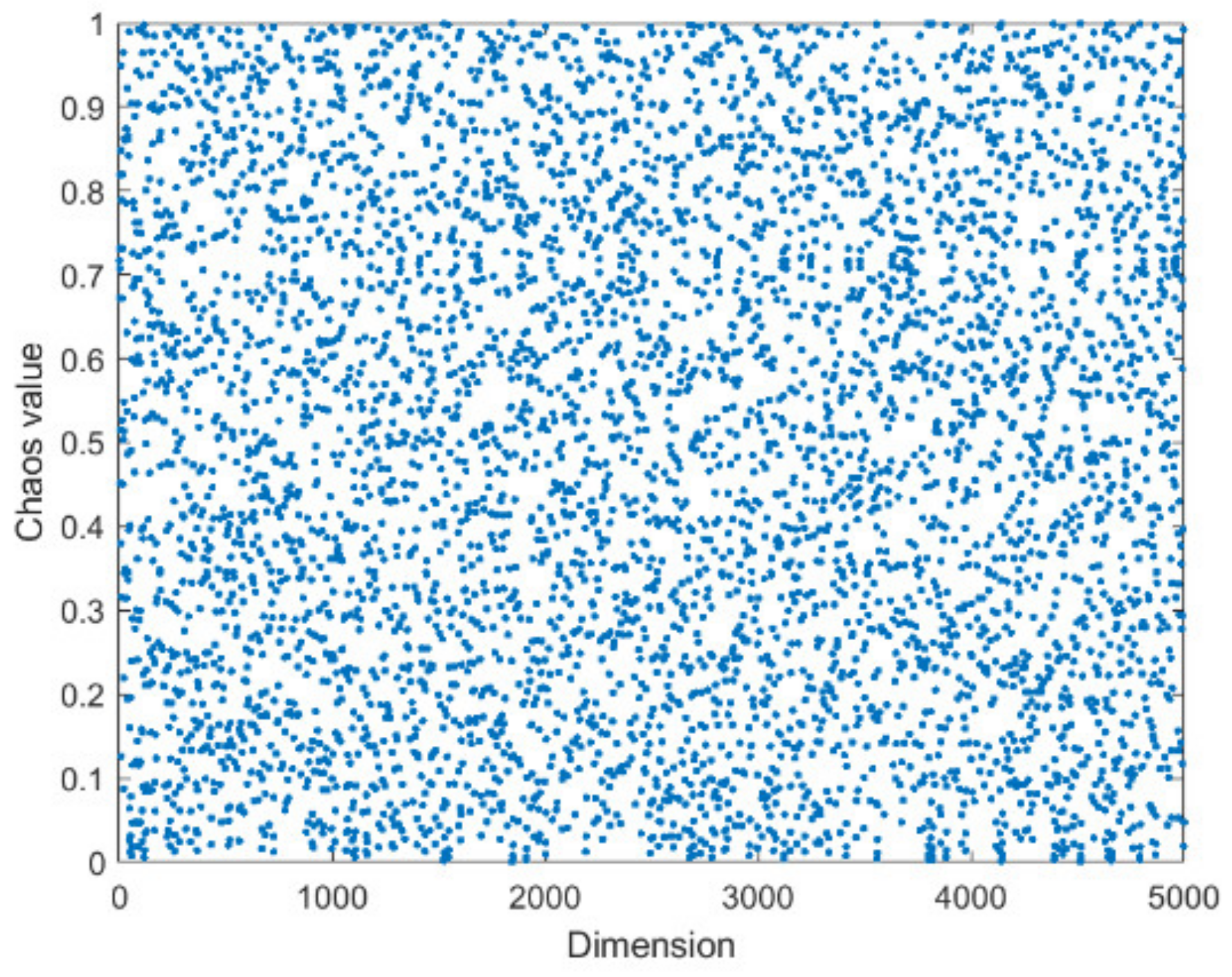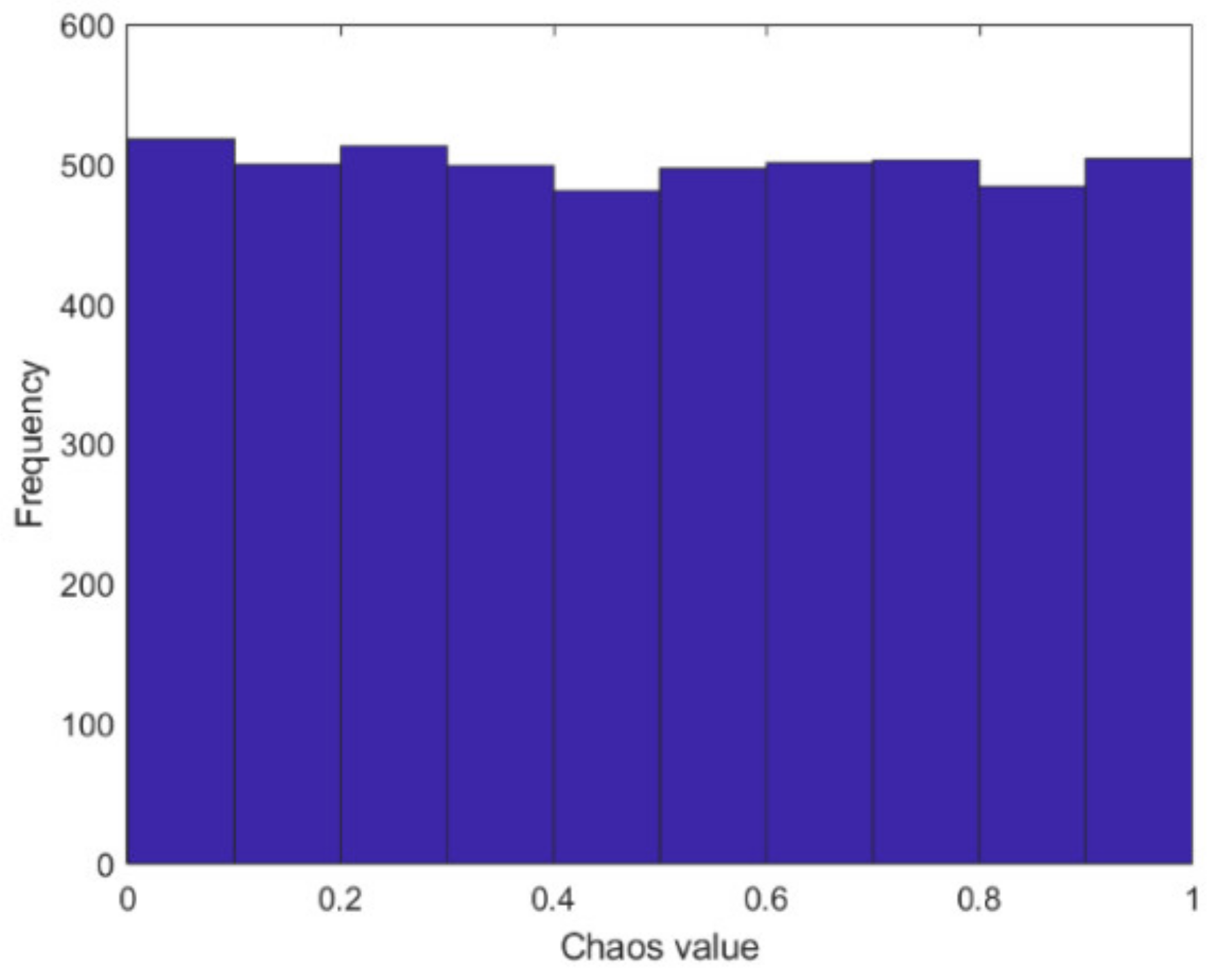Kaur and Arora [40] introduced chaos theory into the optimization process of the WOA. These improved strategies are mainly reflected in the aspects of population initialization, adaptive weights, and local variation. These improved strategies have improved the performance of the WOA to a certain extent, but their effectiveness in solving the location problem remains to be verified.

At present, although some progress has been made in the research on charging demand prediction and site selection, they are all based on their own characteristic parameters and assumptions. Too many assumptions can make the end result too idealistic.

Above all, this paper proposes a charging station location optimization model considering dynamic charging demand and carbon emissions. The contributions of this paper are as follows:

(1)

At present, most of the research on the location of charging stations does not fully understand the charging demand of each station, and it is difficult to satisfy the interests of all parties. Therefore, this paper considers the influence of dynamic charging demand on site selection when establishing the location model.

(2)

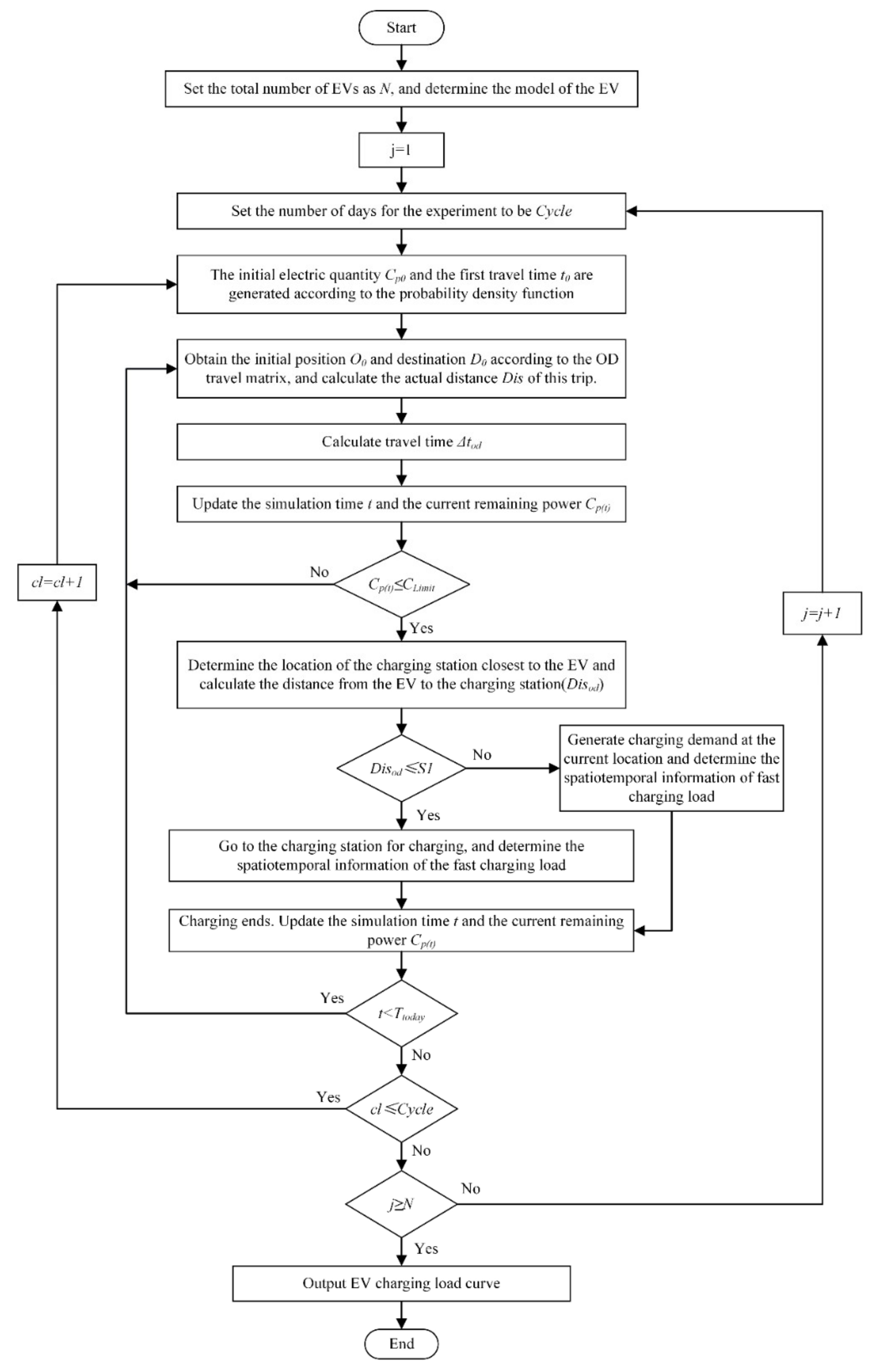
A forecasting model of electric vehicle charging demand based on travel chain data is constructed. Through the analysis of vehicle trajectory, the characteristic parameters of vehicle travel and charging are obtained, and the charging model of a single electric vehicle is constructed. In order to better simulate the daily driving state of the vehicle, this paper fully considers the influence of various uncertain real factors on the simulation.

(3)

A site selection model aiming at the minimum comprehensive cost was established. The impact of different siting options on carbon emissions was explored. We further analyzed the influence of replacing electric vehicles with fuel vehicles on carbon emissions under the same conditions.

(4)

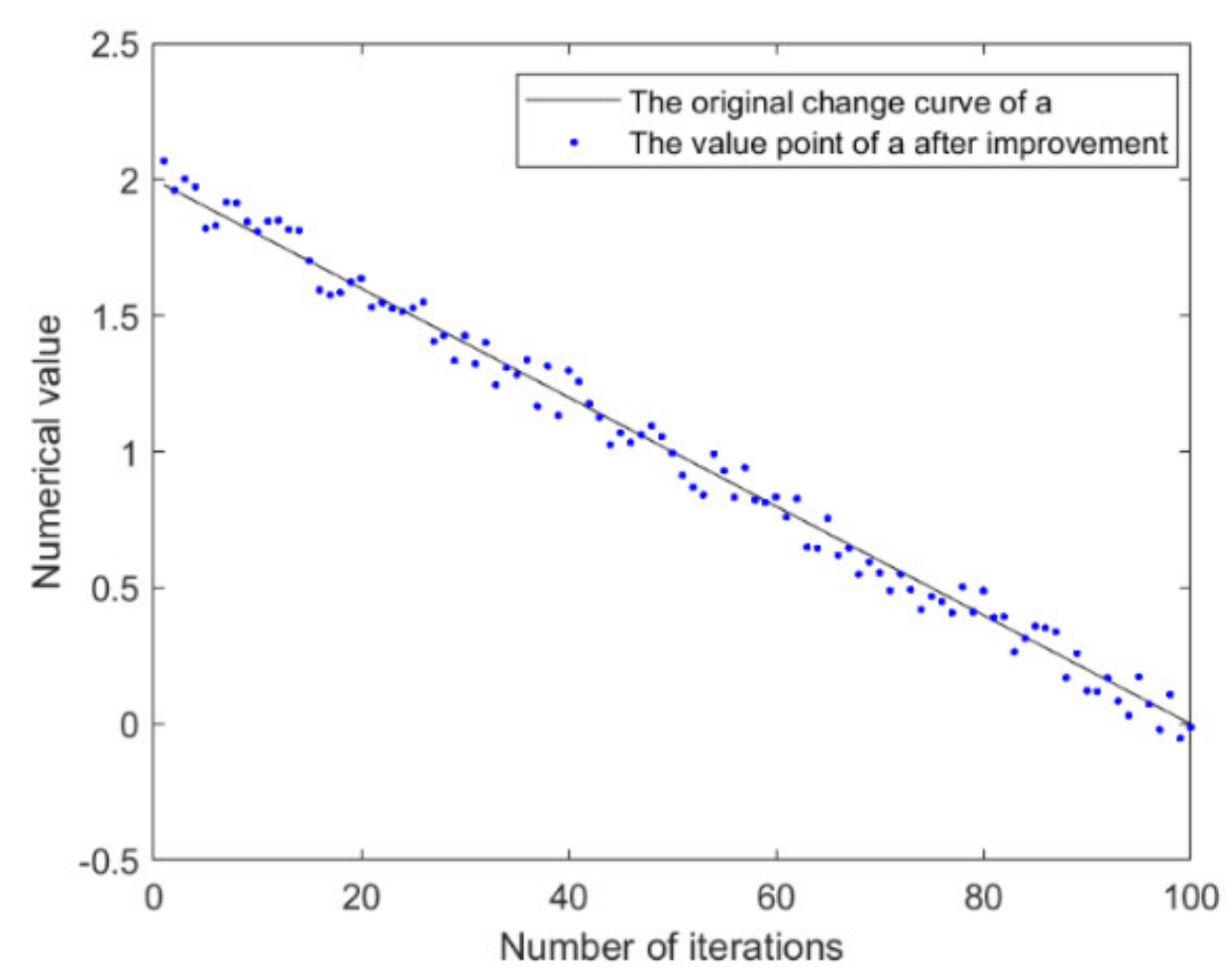
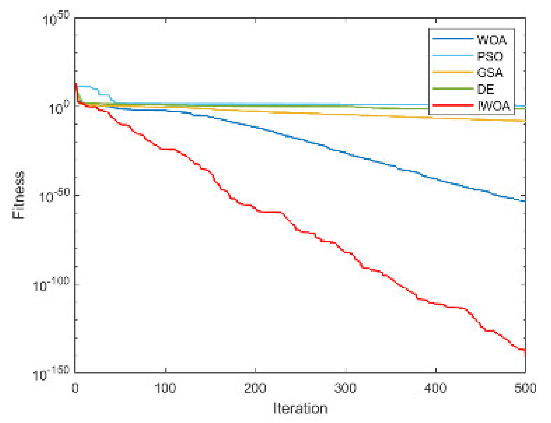
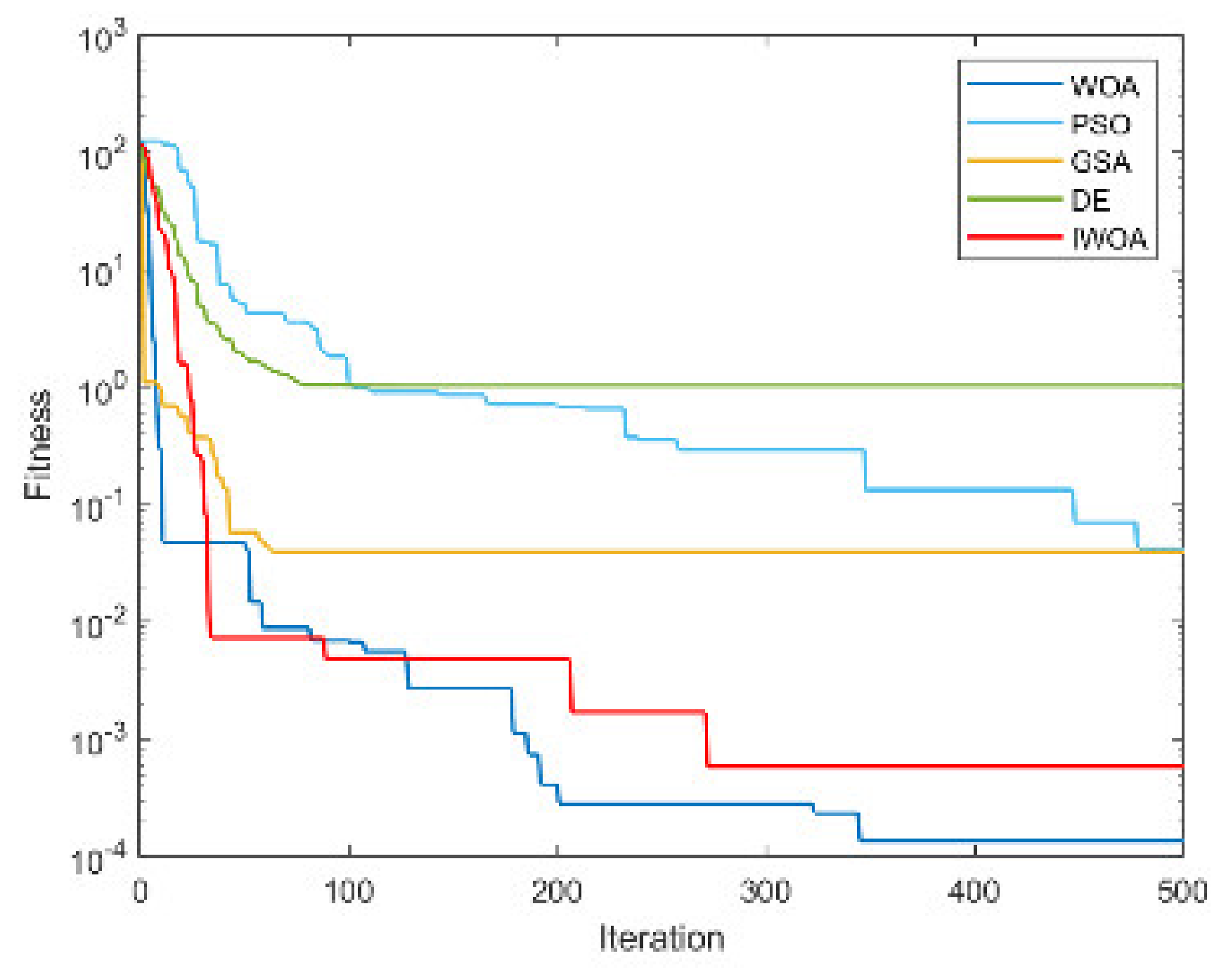
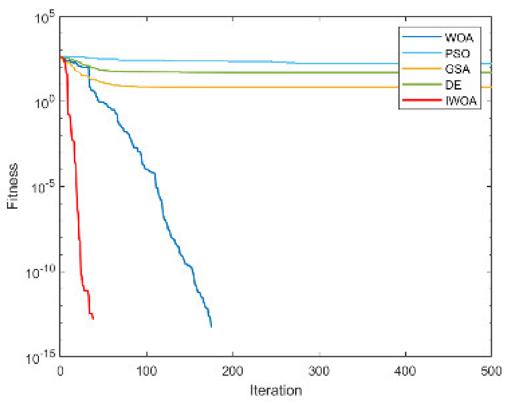
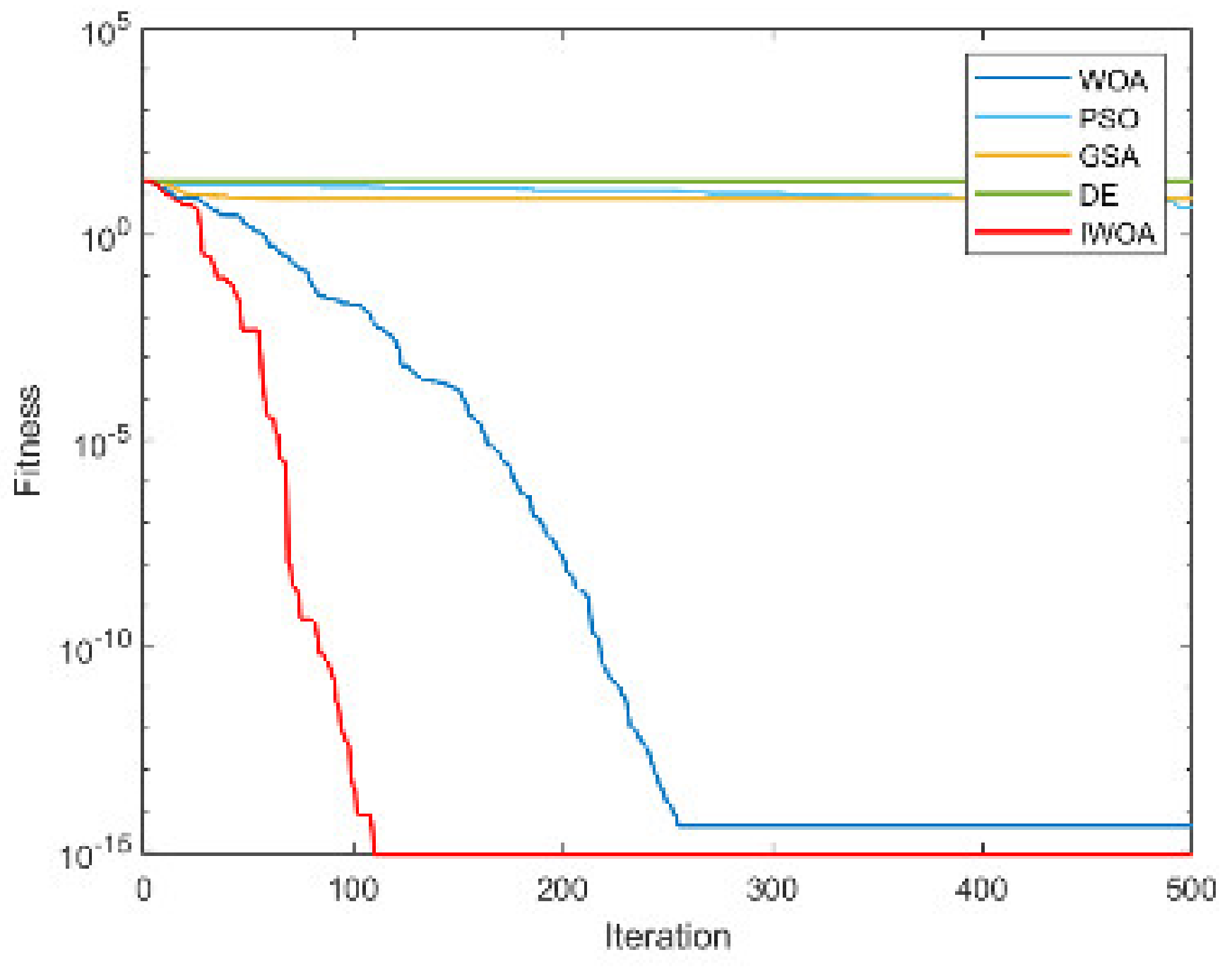
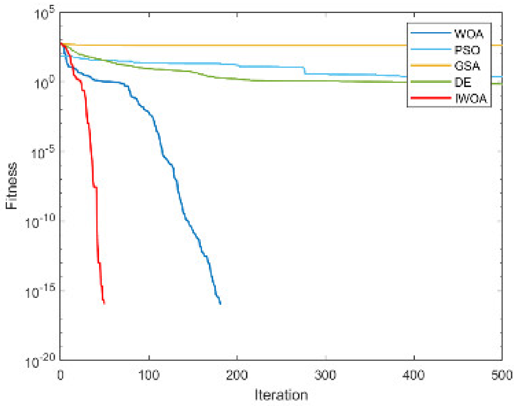
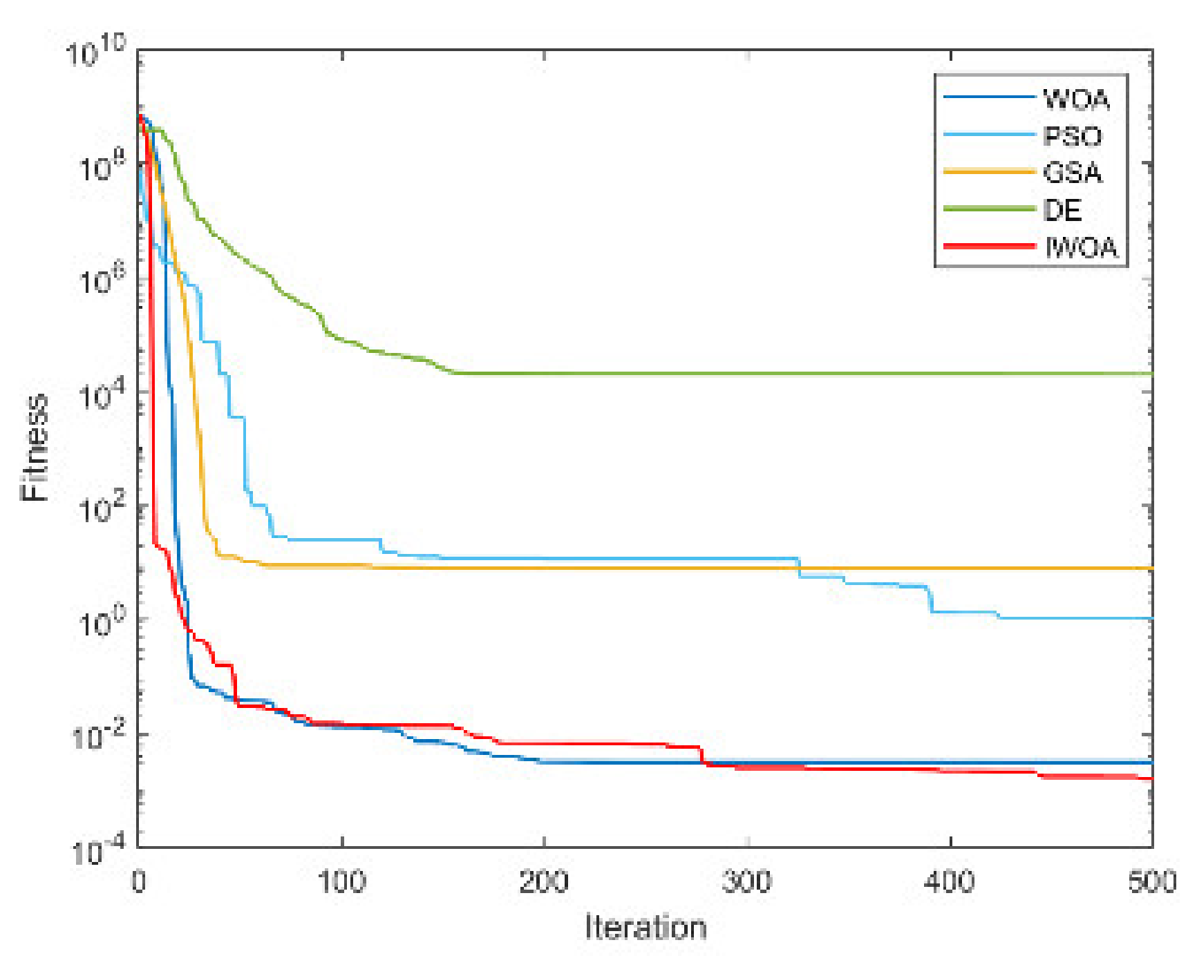
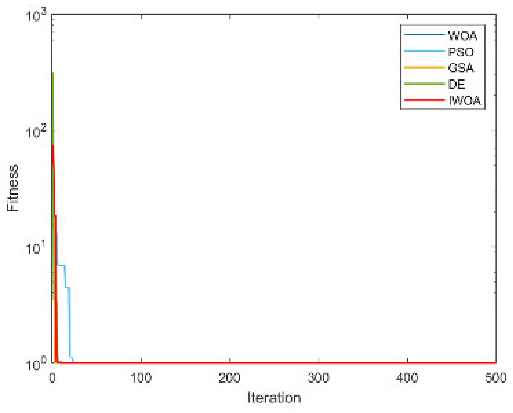
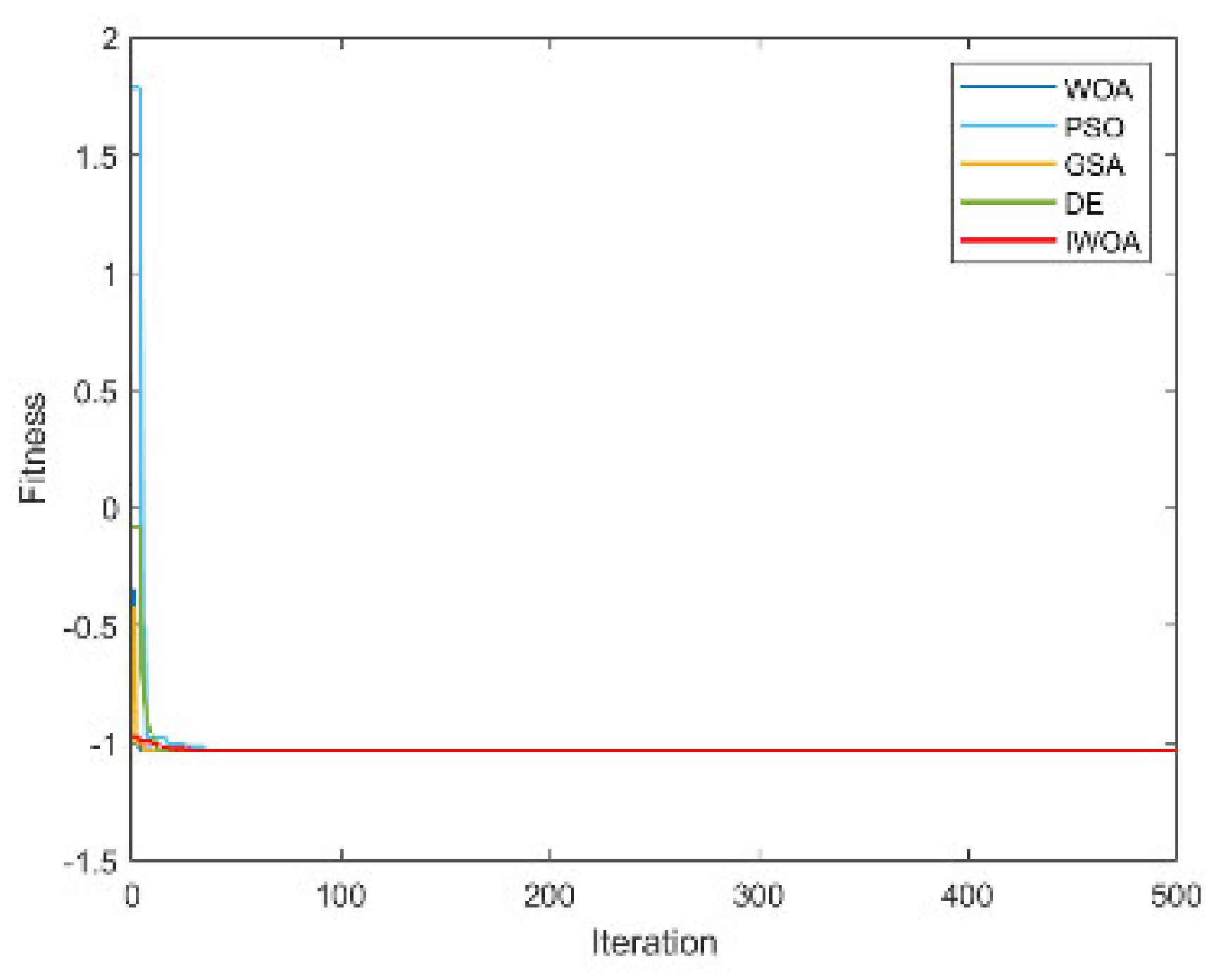
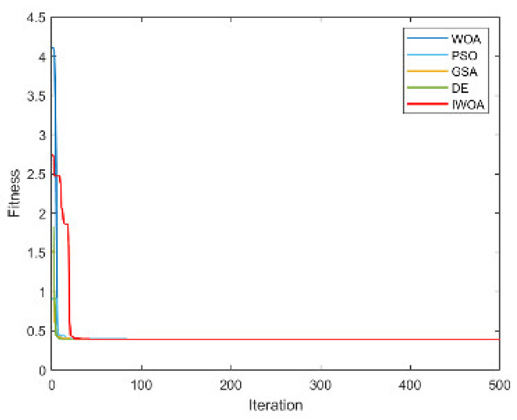
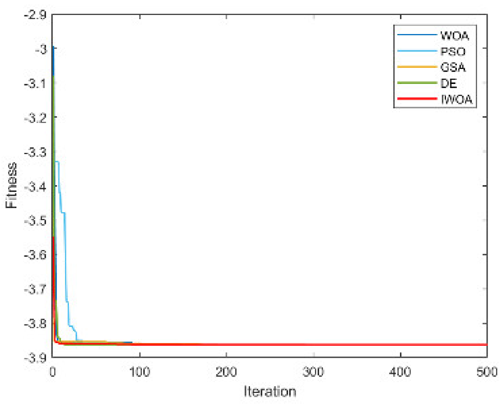
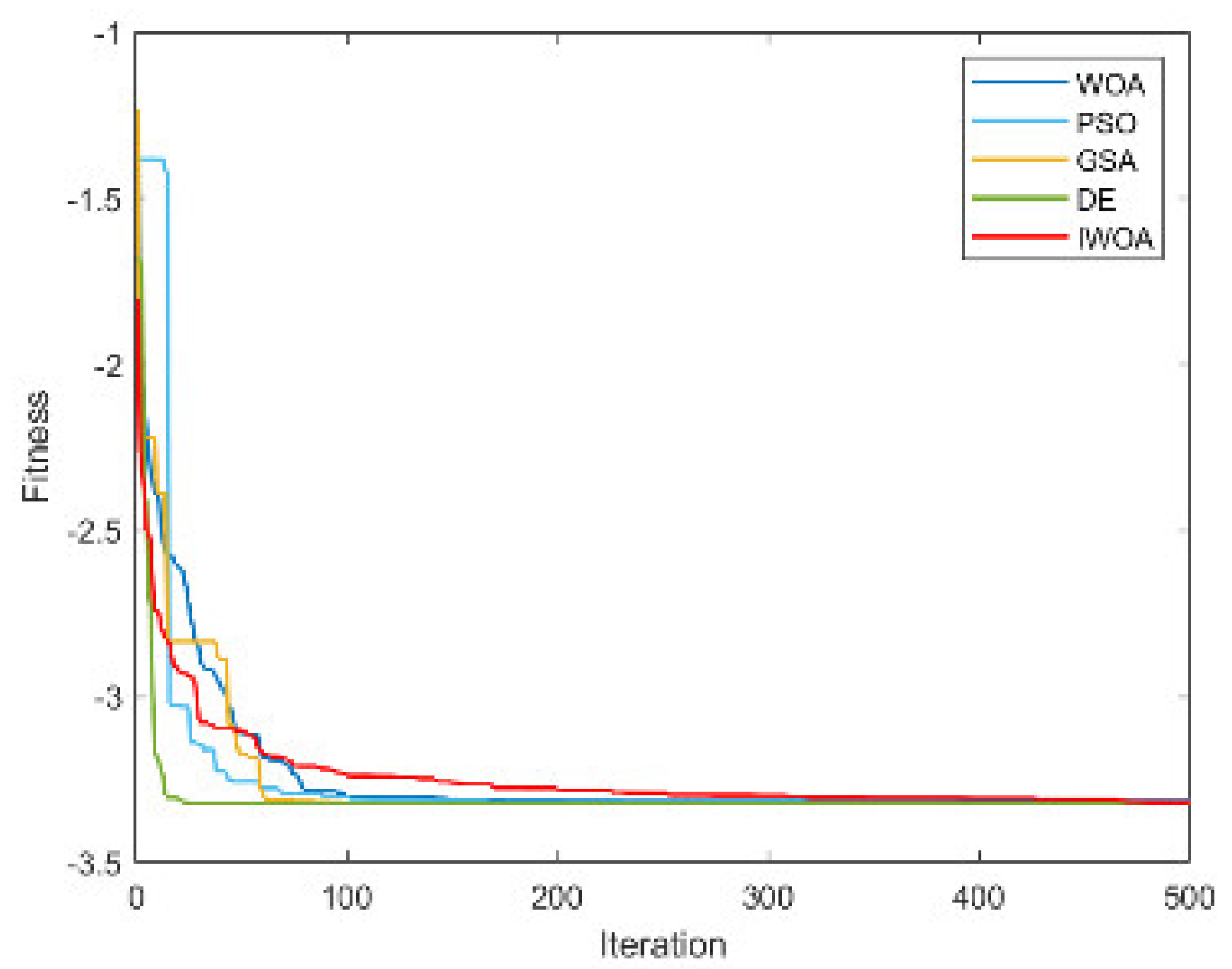
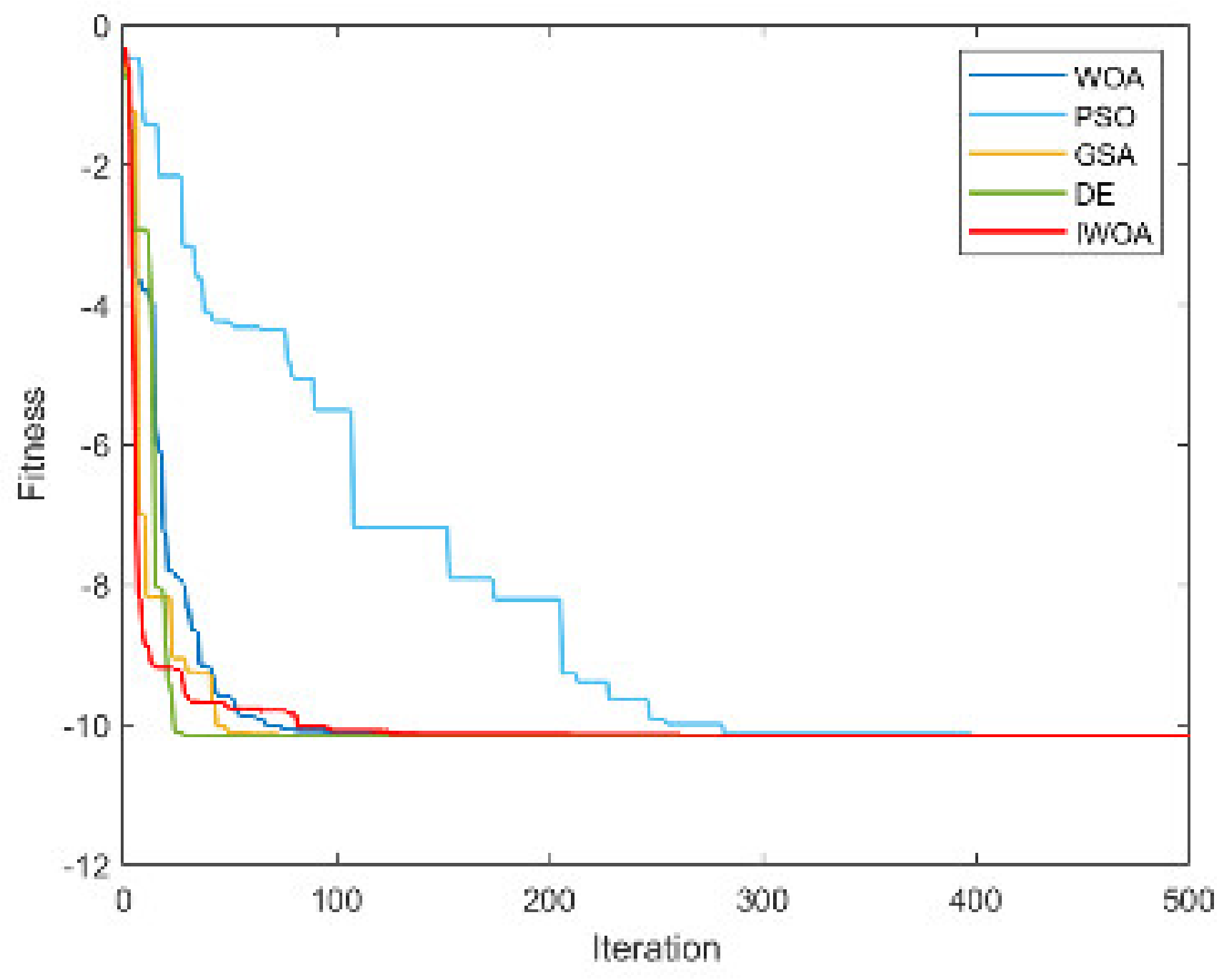
The whale optimization algorithm is improved from four aspects. The effectiveness of the improved algorithm is analyzed by reference test function and location model.

The paper is organized as follows. Section 2 introduces the data processing process and constructs the OD travel matrix; Section 3 introduces the charging station location optimization model; Section 4 introduces the solution method of the location model and the improvement of the whale optimization algorithm; and Section 5 contains the case analysis. The last section is a summary of the thesis.

2. Data Description and Preprocessing

2.1. Data Description and Preprocessing

This study uses open data provided by Rutgers University Assistant Professor Desheng Zhang’s research group for analysis and processing [41]. This dataset contains 1,155,654 GPS records of 664 electric taxis located in Shenzhen, China, on 22 October 2014.

Table 1. Description of the data format of electric taxi trips in Shenzhen.

Field Name	Field Type	Data Example
Vehicle Id	Varchar	0
Longitude	Flout64	114.031799°
Latitude	Flout64	22.524799°
Time	Datatime	2014-10-22T02:54:30.000Z
Speed	Int64	42 km/h

shows the data content:

In addition, the passenger-carrying state of the vehicle can be judged by the change in the driving speed and the track point time. Compared with the study of fuel vehicles trajectory, there are many advantages of using electric taxi trajectory analysis. Currently, electric taxi drivers in Shenzhen can also take orders online. Therefore, to a certain extent, the city’s taxis can be regarded as online car-hailing. Since most network car services can provide point-to-point services, the user’s travel purpose is relatively clear. Compared with traditional taxis, electric taxis that can take orders online will have a lower no-load rate and less redundant data in the data set. The origin-destination (OD) travel matrix constructed according to its trajectory is also more in line with the travel laws of modern residents.

In order to avoid the interference of the noise data in the original data set with the experimental results, the original data need to be preprocessed. Pre-processing includes two parts: time format conversion and cleaning of damaged data. The following data were mainly deleted: data with missing values, data not within the scope of Shenzhen, data with a passenger-carrying distance of less than 500 m, data with a stationary time of less than 60 s, etc.

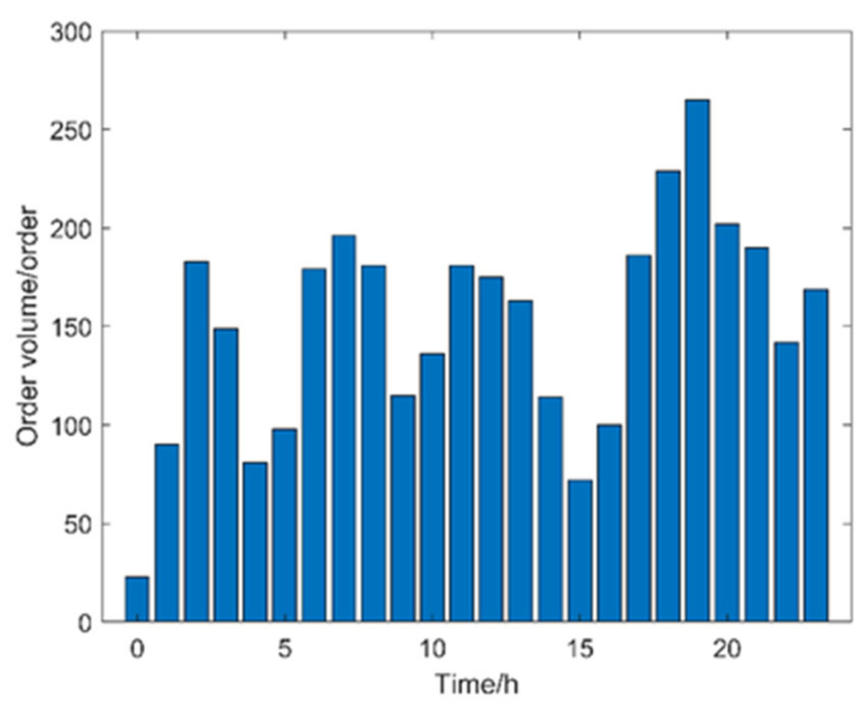
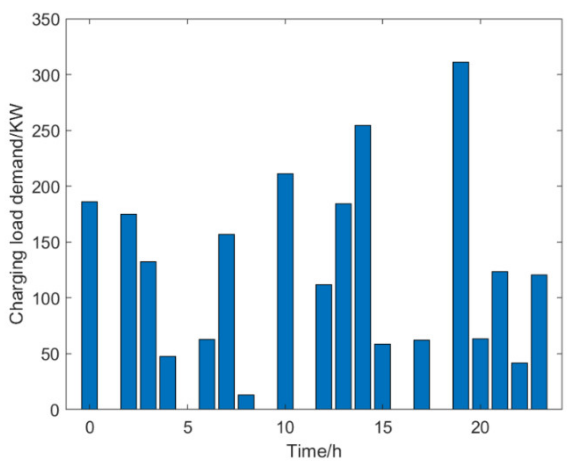
After the data preprocessing was completed, the data were visualized. Figure 1 shows the change in order volume at different times during the day. As can be seen from Figure 1, the order volume shows multiple peaks within a day, and the change curve shows a wavy distribution. At 0:00, the order volume is the least, with only 23 orders. We have analyzed this from two aspects: taxi drivers mostly change shifts at about 0:00, and the evening peak is about to end. At 19:00, the number of orders reached a peak of 269 orders due to the off-duty peak period and at night.

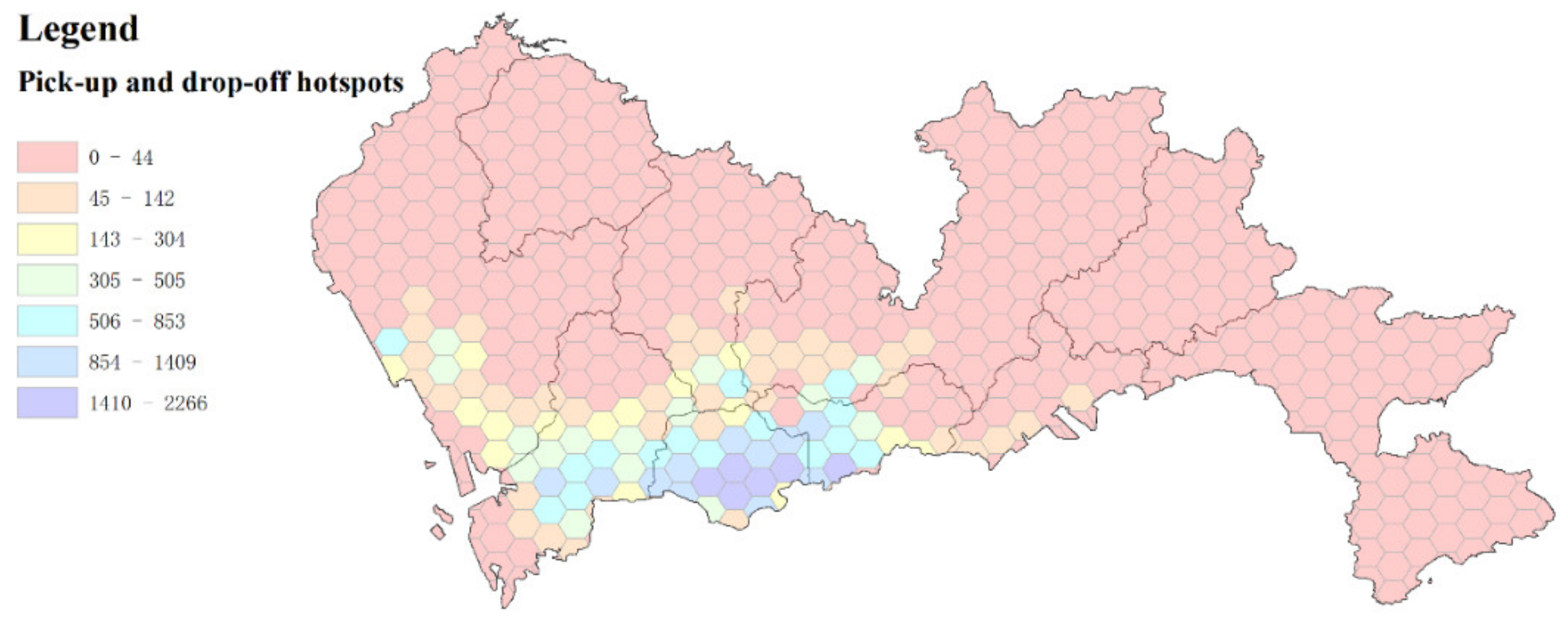
Next, we visualized the pick-up and drop-off points for passengers throughout the day.

As can be seen in Figure 2, hot spots are mainly concentrated in coastal areas such as Nanshan District. Luohu District is adjacent to Hong Kong. It can be seen that the geographical areas along the coast or near international cities are very attractive to tourists.

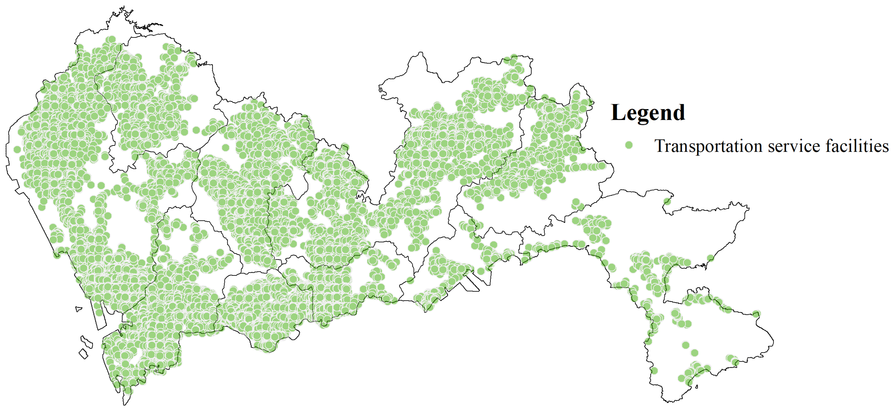
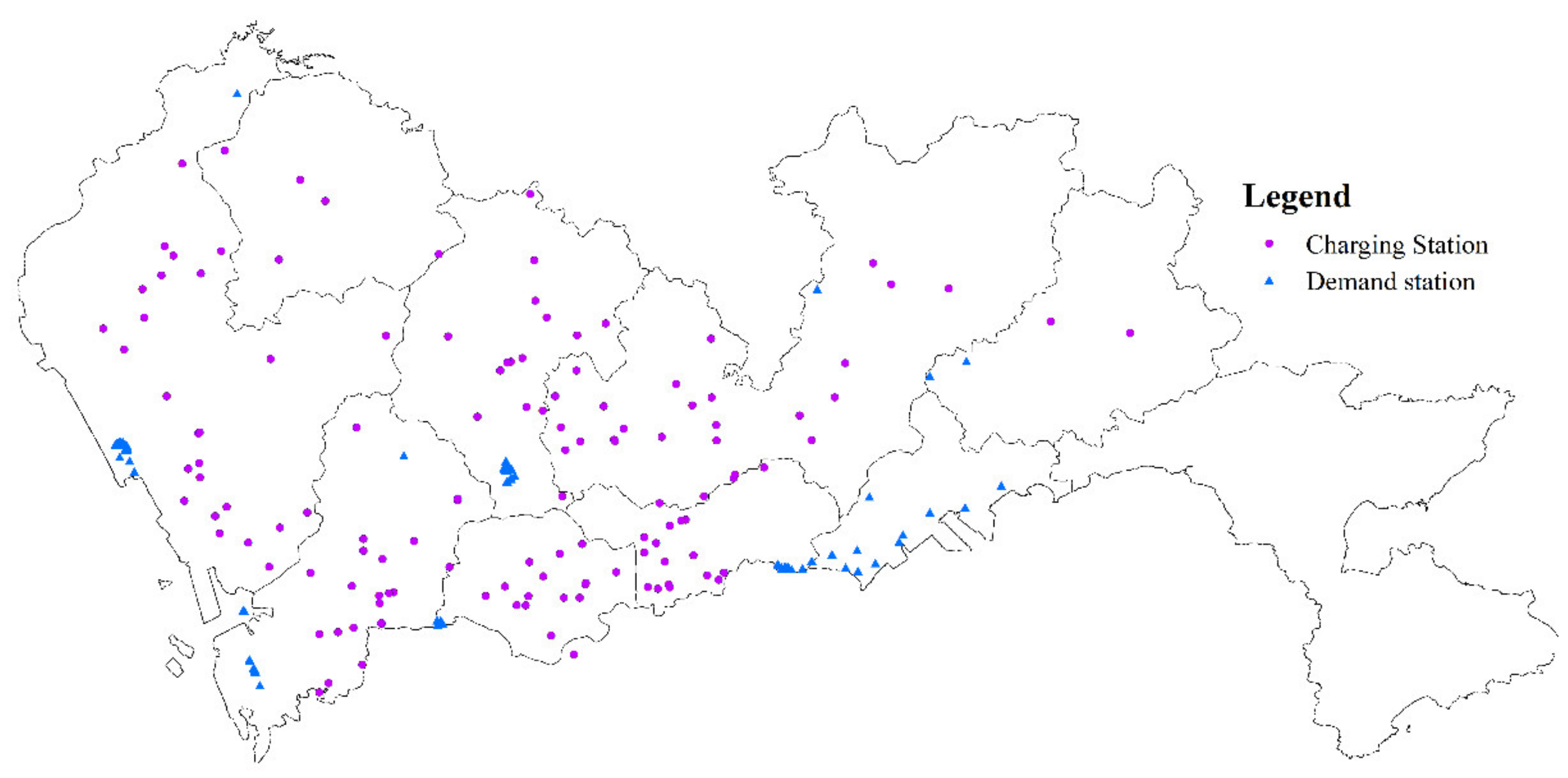
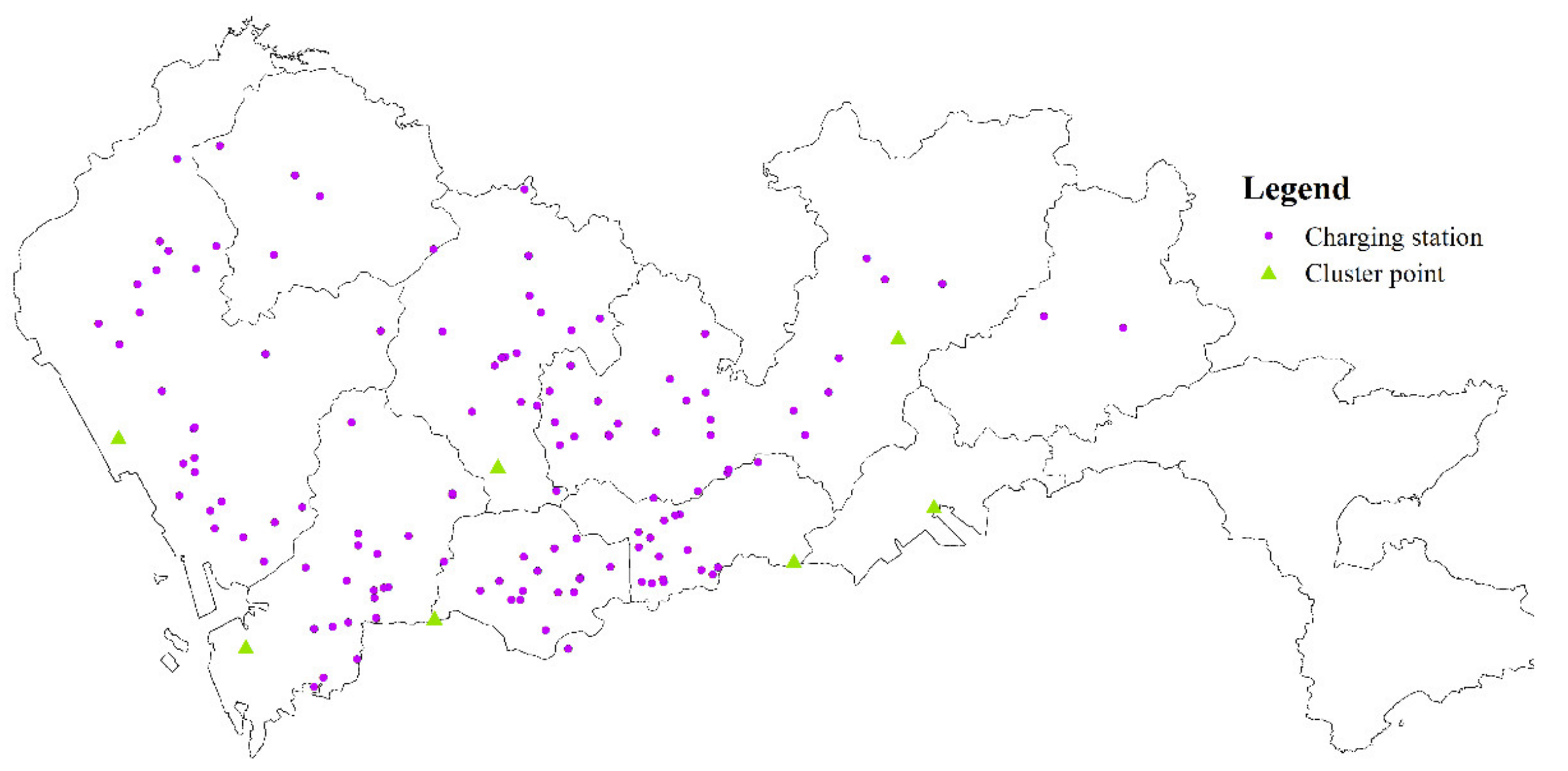
In order to have an intuitive understanding of Shenzhen’s traffic service level, we visualized the location distribution of Shenzhen’s traffic infrastructure, as shown in Figure 3. The green dots represent transportation infrastructure. As can be seen from the figure, more facilities are found in the west than in the east.

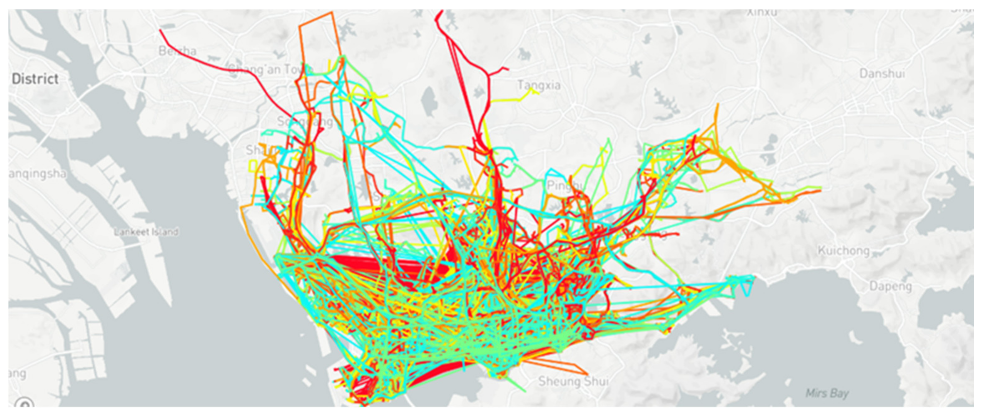
Figure 4 shows the driving tracks of 664 taxis in one day. It can be seen from the figure that the hot activity areas of electric taxis are basically the same as the hot spots for getting on and off.

2.2. The OD Travel Matrix

The origin-destination (OD) travel matrix reflects the travel information of residents or vehicles between the starting point and the ending point. The OD matrix is often used to describe the characteristics of vehicle travel distribution [42]. According to the OD matrix, the travel characteristics of various types of electric vehicles in the urban road network can be described.

The moving position data includes longitude, latitude, time, and other information [8]. In $\left(x_i,y_i,t_i\right)$, $x_i$ and $y_i$, respectively, represent the longitude and latitude of point i of the travel trajectory $\Omega$, and $t_i$ represents the time of point i, $i=1,2,\dots ,n$, then the trajectory $\Omega$ can be expressed as: $\Omega =\{\left(x_1,y_1,t_1\right),\left(x_2,y_2,t_2\right),\left(x_3,y_3,t_3\right),\dots ,\left(x_n,y_n,t_n\right)\}$.

In order to facilitate the rapid statistics of traffic demand in the grid, the longitude and latitude of traffic demand location points are converted into grid numbers. Through the analysis of the grid, the traffic demand in the grid can be calculated indirectly. The grid division method involved dividing the study area into equal squares at a certain interval. The partition interval is denoted by W. When W is 0.01, it means that the research area is divided into several grids of equal size with an interval of 0.01°. In the longitude direction, when the two points are separated by 0.01°, the actual distance is about 900 m. When the two points are separated by 0.01° in the latitude direction, the actual distance is about 1100 m.

$\left(X_{\min },Y_{\min }\right)$ is defined as the coordinates of the lower left corner node of the research area grid, $\left(X_{\max },Y_{\max }\right)$ is the coordinates of the upper right corner node of the research area grid, and $\left(X_i,Y_i\right)$ is the latitude and longitude coordinates of any node in the grid. $\left(Gri{d}_x,Gri{d}_y\right)$ is the number of the grid where $\left(X_i,Y_i\right)$ is located, and the grid node number is $G_{xy}$.

$$Gri{d}_x=\mathrm{int}((X_i-X_{\min })/W)$$

(1)

$$Gri{d}_y=\mathrm{int}((Y_i-Y_{\min })/W)$$

(2)

$$G_{xy}=Gri{d}_x+Gri{d}_y·72$$

(3)

The latitude and longitude range of the pre-processed taxi data: longitude from 113.68° to 114.4°, latitude from 22.46° to 22.88°.

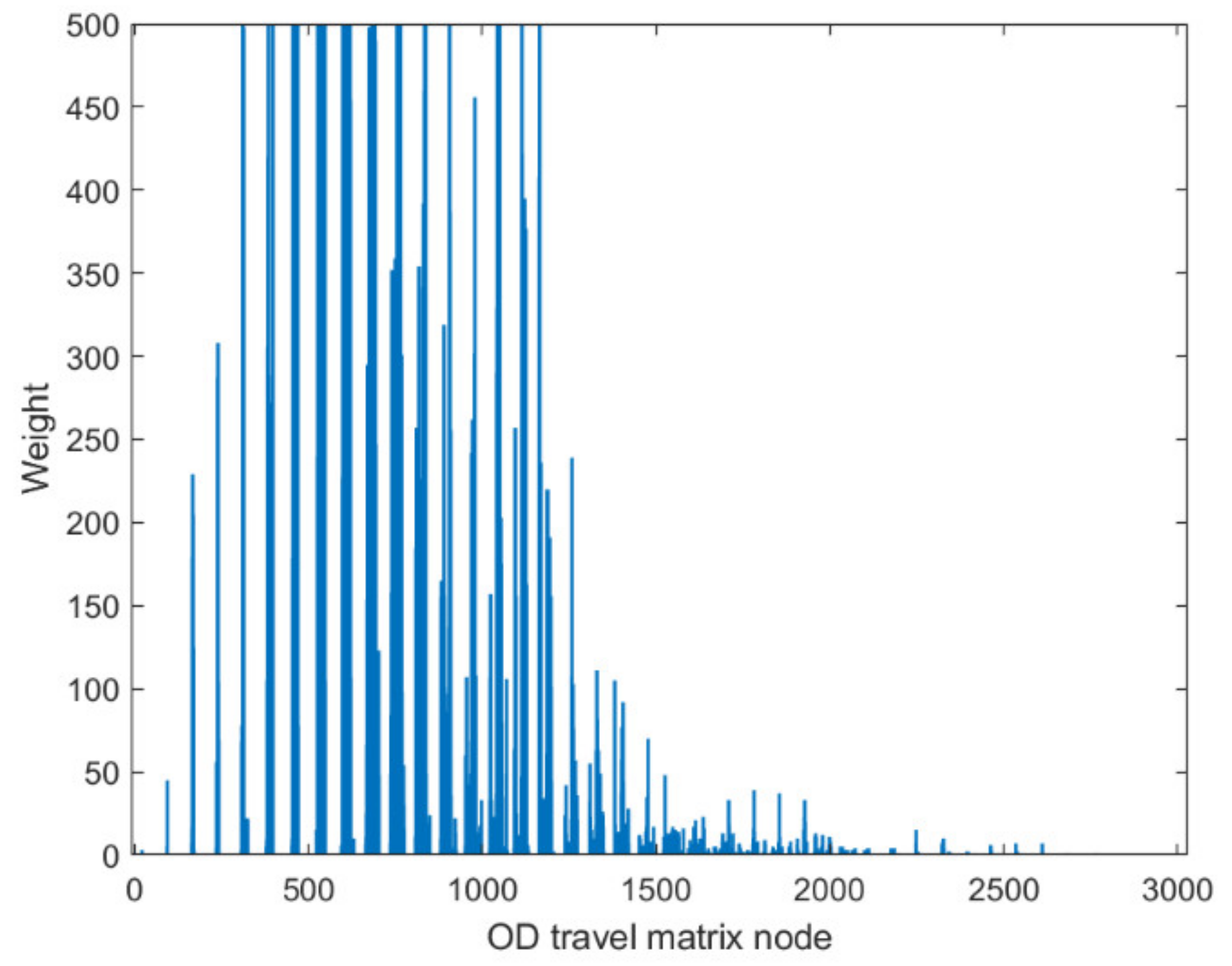
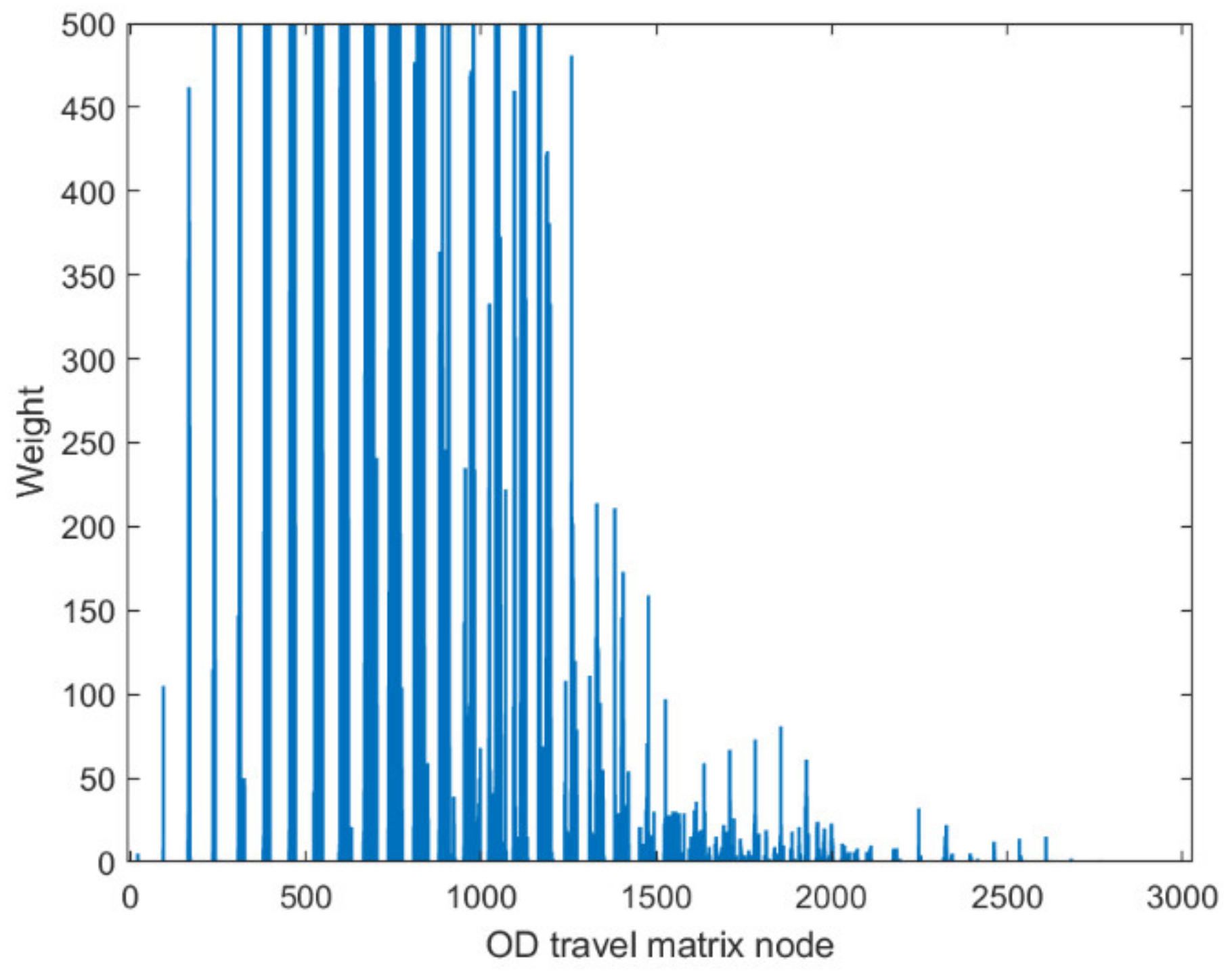
After the division of latitude and longitude, it can be seen that there are 3024 nodes in total. There are 11,328 OD pairs in total. The traffic volume between two nodes is calculated by:

$$tri{p}_{rs}={\displaystyle \sum _r{\displaystyle \sum _s{f}_{rs}}}$$

(4)

where $r$ is the starting point of a pair of OD pairs, and $s$ is the end point of an OD pair. $f_{rs}$ is the number of paths from the starting point to the ending point. $tri{p}_{rs}$ is the traffic volume between two nodes.

3. Electric Vehicle Charging Station Site Selection Model

3.1. Electric Vehicle Charging Demand Forecasting Model

3.1.1. Vehicle Parameters

In order to further implement the concept of green development, the Shenzhen Municipal Transportation Bureau steadily promotes the work of pure electric taxis and basically achieved the goal of full-electric electrification in 2018. Shenzhen has become the only city in China to realize pure electric taxis, and it is also the city with the largest number of pure electric cruisers operating in the world. The data shows that this city with a population of about 12 million has turned to electric transportation on a large scale. At present, the taxi model mainly used in Shenzhen is BYD e6. The vehicle parameters are shown in

Table 2. Basic parameters of BYD e6.

Vehicle Model	BYD e6
Pure electric cruising range (km)	400
Fast charge time (h)	1.5
Slow charge time (h)	8
Maximum power (kW)	120
Top speed (km/h)	140
Battery power (kWh)	82
Battery Type	Lithium iron phosphate battery
Motor type	DC

:

3.1.2. Start Travel Time and Initial SOC

Electric taxi charging demand is mainly influenced by the daily mileage and travel time of electric taxis. The starting travel time of electric taxis affects the charging demand at different times of the day. According to the statistical data provided by the National Cooperation Highway Research Program [43], the probability distribution curve of the starting travel time $t_0$ of electric vehicles can be obtained after fitting. The probability distribution curve of the initial travel time of electric taxis is shown in Figure 5.

This paper assumes that the state of charge (SOC) of the battery when the electric vehicle travels for the first time obeys the normal distribution $N_{SOC}(0.8,0.1)$. According to the parameters in Table 2, it can be seen that the battery capacity is $carPower=82kwh$. Through Equation (5), the amount of electricity at the first trip can be calculated as $C_{P0}$. Where $SO{C}_{Star}$ is the initial SOC.

$$C_{P0}=SO{C}_{Star}·carPower$$

(5)

The power consumption of electric taxis increases with the mileage. Using Equation (6), the remaining power of the electric taxi at the time t can be calculated.

$$C_{p(t)}=\eta ·(SO{C}_{t-1}-SO{C}_t)·carPower$$

(6)

Among them, $C_{p(t)}$ is the battery power at time $t$. $SO{C}_{t-1}$ is the state of charge of the battery at the time $t-1$. Considering the energy loss caused by braking and other factors during driving, the energy coefficient $\eta$ is introduced, and the value range is 0.9~1.

3.1.3. Charging Duration

At present, all the electric taxis in Shenzhen use fast charging [8]. When the power of the charging pile is 60 kW, it takes about 1 h and 22 min for an electric taxi with 0 remaining power to be fully charged. According to the driving characteristics of taxis, the minimum charging time is considered to be satisfied when the interval from the end of the last trip to the beginning of the next trip exceeds 15 min. According to the set parameters, charging for 15 min can supplement the electric vehicle with 15 kilowatts of electricity. With a range of 400 km, 15 kW would give an electric taxi a range of about 73 km.

The no-load time data of electric taxis are extracted from the preprocessed data. With the help of the MATLAB (R2020a) distribution fitter, we can quickly check the distribution of the data. When fitting the probability distribution of the data, we choose a non-parametric distribution. The result of its probability fitting distribution is shown in Figure 6. The data were fitted with the help of MATLAB’s cf tool. First, we select the type of fitting curve as Gaussian. Then we keep changing the number of terms and observe the data fitting observations. If the result is suitable, we fit it several times to reduce the error; if the result is not suitable, we choose another way to fit it. Finally, it was found that when the number of items is 2, the result is more reasonable, as shown in Figure 7:

From the fitting process, we can see that when Gaussian is used to fit the charging duration relationship, it conforms to the relevant criteria in data fitting: SSE = 0.003127, R−square = 0.9968. The expression is:

$$f(x)=0.004781·\exp (-{((x-73.84)/17.98)}^2)+0.01294·\exp (-{((x-62.26)/36.74)}^2)$$

(7)

In Equation (7), $x$ is the time when the electric taxi is in an empty state, and $f(x)$ is the corresponding probability value. As can be seen from Figure 7, the time when electric taxis are in an empty state is mainly concentrated in 15 min to 100 min, and the probability is highest at 70 min. When the taxi is fully charged, it takes an hour and 22 min. In Figure 7, the empty time of an electric taxi has a certain probability of obtaining a value greater than 1 h and 22 min. At this time, times exceeding 1 h and 22 min are invalid for charging electric taxis, so the actual charging time of an electric taxi is:

$$Act=\{\begin{array}{l}x/60\hspace{1em}\hspace{1em}\hspace{1em}{t}_{need}>x/60\\ t_{need}\hspace{1em}\hspace{1em}\hspace{1em}{t}_{need}\le x/60\end{array}$$

(8)

$$C_{use}=C_{p0}-C_{p(t)}$$

(9)

$$t_{need}=C_{use}/P_{ch\arg }$$

(10)

Among them, $C_{use}$ is the electricity consumed by the electric taxi. $P_{ch\arg }$ is the power of the charging pile, $P_{ch\arg }=60 kW$. $t_{need}$ is the time required for the electric taxi to be fully charged from the current charge.

3.1.4. Judgment of Charging Status

Generally speaking, electric taxi drivers will not wait until the remaining battery capacity of the vehicle is 0 before recharging. When the electric quantity of the taxi is lower than the set threshold electric quantity $C_{Limit}$ at a certain time, the charging demand is generated:

$$C_{p(t)}\le \epsilon ·C_{P0}$$

(11)

$\epsilon$ is the user’s mileage anxiety coefficient, which obeys uniform distribution, and its expression is as follows:

$$f(\epsilon )=\{\begin{array}{l}1/(b-a)\hspace{1em}a<\epsilon <b\\ 0\hspace{1em}\hspace{1em}\hspace{1em}\hspace{1em}\hspace{1em}else\end{array}$$

(12)

Figure 8 shows the charging process of a taxi. There are four taxis driving on the road in Figure 8. CS1, CS2, and CS3 are charging stations in Figure 8. CS1 is close to CS3. The circle represents the service range of the charging station. S1 represents the charging service range of a charging station. S2 represents the distance between two charging stations.

In the process of driving, when the driver finds that the cruising range of the taxi is small and it will be difficult to complete their next trip, there will be charging demand. Generally speaking, when the charging demand is triggered, the driver will choose to charge at the nearest charging station and generate the space-time information of a fast charging load. Figure 8 is a simulation analysis of the charging process of the vehicle. If taxis Car1 and Car2 want to be charged, they can choose to go to the charging station CS2 for charging because they are within the service range of the charging station CS2. If the taxi Car3 needs to be charged, we can see that the distance between Car3 and CS1 or CS2 is the same, so it can choose either CS1 or CS2 when choosing a charging station. When Car4 needs to be charged, we can see that the three charging stations in the figure are far away from Car4. From this, we find that the location of charging stations CS1 and CS2 is not reasonable and objective. Because CS1 and CS2 are close to each other, the intersection of the orange circle and blue circle in the figure is rich in charging resources, which greatly meets the charging demand of this place. However, it brings some problems, such as uneven distribution of charging resources, difficult charging for users, etc. This is not conducive to the charging of taxi Car4 and nearby vehicles. In order to improve this unreasonable situation, this paper sets that when a taxi needs charging, if the distance between the taxi and its nearest charging station is less than S1, it will go to the charging station to charge; otherwise, the current location of the taxi is considered as a potential charging demand point and the time-space information of fast charging load is determined. Meanwhile, the distance between charging stations should be no less than S2.

3.1.5. Charging Demand Forecasting Model Based on the Monte Carlo Method

The Monte Carlo method is used to calculate the charging load of electric taxis. The starting travel time $t_0$ and the initial SOC $SO{C}_{Star}$ are randomly generated according to the probability density function. According to the OD matrix, each electric vehicle is assigned an initial position $O_i$ and a destination $D_i$. Combined with the pre-set charging mode, electric vehicle type, and other data, it is possible to simulate the journey of an electric taxi for a day. Finally, the spatiotemporal distribution of the charging demand of electric taxis for one day is obtained. The electric taxi charging demand forecasting process is shown in Figure 9.

3.2. Charging Station Site Selection and Capacity Model

Electric vehicle charging stations are public service facilities. When planning a charging station, we should consider not only the interests of the enterprise but also the charging experience of users. In this study, considering the constraints of charging service range, charging coverage rate, and charging station scale, a mathematical model to minimize the comprehensive cost was established.

3.2.1. Objective Function

The objective function of the location model consists of three parts: annual construction and operation cost $F_{C1}$, time cost $F_{C2}$, and penalty term $F_{C3}$. In addition to cost considerations, we also consider the carbon footprint of electric taxis on the way to the charging station as an important consideration. $Carbo{n}_{ijk}$ is the carbon dioxide emissions generated by electric taxis during the trip, as shown in Equation (14). In order to understand the impact of different power systems on carbon emissions, this paper also compares the carbon emissions produced by electric vehicles and gasoline vehicles under the same driving range. $Carbo{n}_{ijk}^{fuel}$ is the carbon dioxide emissions generated by fuel taxis during the trip, as shown in Equation (15).

$$\min F=F_{C1}+F_{C2}+F_{C3}$$

(13)

$$Carbo{n}_{ijk}=\omega ·d_{ijk}·W_a$$

(14)

$$Carbo{n}_{ijk}^{fuel}=\zeta ·d_{ijk}$$

(15)

In Equation (14) and Equation (15), $d_{ijk}$ represents the distance of the vehicle $k$ from the starting point $i$ to the end point $j$. $W_a$ represents the power consumption rate of an electric vehicle. $\omega$ denotes the CO₂ emission rate of using electricity, and $\zeta$ is the CO₂ emission rate of using gasoline.

The $F_{C1}$ includes the annual construction cost $C\mathrm{on}$ and the annual operation cost $Cop$. Construction costs mainly include charging piles, land, transformers, etc., as shown in Equation (16).

$$C\mathrm{on}=\frac{r_0·{(1+r_0)}^{nyear}}{{(1+r_0)}^{nyear}-1}·(Cg+\phi ·ncha{r}^2+\epsilon ·nchar)$$

(16)

In Equation (16), $r_0$ is the discount rate. $nyear$ represents the depreciation life. $Cg$ is the fixed investment cost. $nchar$ represents the number of charging piles in the charging station. $\phi$ represents the equivalent investment factor for the cost of related equipment such as distribution transformers and transmission lines. $\epsilon$ is the price of a single charging pile.

Operating costs include labor costs, equipment maintenance costs, and other expenses, as shown in Equation (17). Where $\gamma$ is the conversion factor of running cost, $\gamma =0.1$. $F_{C1}$ can be obtained by Equation (18).

$$Cop=(Cg+\phi ·ncha{r}^2+\epsilon ·nchar)·\gamma$$

(17)

$$F_{C1}={\displaystyle \sum _{i\in M}(Co{n}_i+Co{p}_i)}$$

(18)

The time cost mainly considers the cost spent by the user on the way to the charging station. $F_{C2}$ can be obtained by Equation (19).

$$F_{C2}=365·\cos tF·\lambda$$

(19)

Among them, $\cos tF$ represents the distance from the demand point to the corresponding charging station. $\lambda$ is the amount spent by the electric vehicle to travel 1 km.

The penalty term $F_{C3}$ represents the cost incurred due to not satisfying the constraint. It can act as a disincentive for sites that do not satisfy the constraint.

$$F_{C3}=Cf1+Cf2+Cf3$$

(20)

$$Cf1=365·1.79·C_a$$

(21)

$$Cf2=C_b/2·15,000$$

(22)

$$Cf3=C_c·10,000$$

(23)

Demand points and charging stations constitute a demand distribution relationship. If the distance of the trip corresponding to this pair of relationships exceeds $S1$, the distance value will be stored in the set $S_a$. $C_a$ is the sum of all distance values in the set $S_a$. In the set of charging service stations, if the distance between the two stations exceeds $S2$, the station is stored in the set $S_b$. $C_b$ represents the number of sites in the set $S_b$. $C_c$ represents the number of stations that cannot meet the demand for charging demand points.

3.2.2. Constraint Condition

(1)

Distance constraint of charging station

The charging demand point should be within the service scope of the charging service station:

$$d_{ij}\le S1$$

(24)

Among them, $d_{ij}$ represents the distance between the charging service station $i$ and the charging demand point $j$.

S2 can affect the utilization rate of charging stations and corporate profits. Its value needs to satisfy the Equation (25). $d_{i_1-i_2}$ indicates the distance between the charging station $i_1$ and $i_2$.

$$\{\begin{array}{l}S2=S1\sqrt{3}\\ d_{i_1-i_2}\ge S2\end{array}$$

(25)

(2)

Distribution relation of charging demand

Equation (26) indicates that a demand station can only be charged by one charging service station. Equation (27) specifies that the number of charging service stations is $p_{station}$. Equation (28) ensures that the demand at the demand point can only be provided by the charging service station. Equation (30) constrains the number of charging stations.

$${\displaystyle \sum _{i\in M_i}{Z}_{ij}}=1,j\in N$$

(26)

$${\displaystyle \sum _{i\in M_i}{h}_i=p_{station}}$$

(27)

$$Z_{ij}\le h_i,j\in N,i\in M_i$$

(28)

$$Z_{ij},h_i\in \{0,1\},j\in N,i\in M_i$$

(29)

$$\mathrm{int}(Q_{\min }/carPower)+1\le p_{station}\le \mathrm{int}(Q_{\max }/carPower)+1$$

(30)

In Equation (26) to Equation (30), $N$ is the set of demand stations. $j$ is the demand station. When the value of $Z_{ij}$ is 1, it means that the demand of station $j$ is provided by charging station $i$, otherwise it is 0. When the value of $h_i$ is 1, it means that point $i$ is selected as the charging station. $Q_{\min }$ is the minimum value of the charging load demand. $Q_{\max }$ is the maximum value of the charging load demand.

4. Location Model Solving

4.1. Whale Optimization Algorithm

The WOA is an algorithm based on the behavior of whales when rounding up their prey [38]. In the process of optimization, it is mainly divided into three stages: search for prey, surround prey, and bubble net attack.

During the hunting phase, each humpback participating in the hunting behavior represents a feasible solution x. The mathematical model of its enveloping phase is:

$$X(t+1)=X_{rand}(t)-A·D$$

(31)

$$D=|C·X_{rand}(t)-X(t)|$$

(32)

$$A=2·a·r_1-a$$

(33)

$$a=2-(2t/Max\_iter)$$

(34)

$$C=2·r_2$$

(35)

where $t$ is the current iteration number. $Max\_iter$ is the maximum number of iterations. $X(t)$ represents the current whale’s position. $X_{rand}(t)$ represents the position of any whale in the hunting group. $r_1$ and $r_2$ are random numbers.

Humpback whales surround their prey when hunting. To describe this behavior, Mirjalili proposed the following mathematical model. $X^{*}(t)$ represents the best whale position so far.

$$X(t+1)=X^{*}(t)-A·D$$

(36)

$$D=|C·X^{*}(t)-X(t)|$$

(37)

Humpback whales swim toward their prey in a spiral motion when attacking their prey with a bubble net. So the mathematical model is as follows. Where $b$ is a constant coefficient. $l$ is a random number in (−1, 1).

$$X(t+1)=X^{*}(t)+D^{’}·e^{bl}·\cos (2\pi l)$$

(38)

$$D^{’}=|X^{*}(t)-X(t)|$$

(39)

4.2. Algorithm Improvement

Aiming to explore the problems of slow optimization speed and low accuracy in the WOA, an improved whale optimization algorithm (IWOA) based on a hybrid strategy is proposed and the effectiveness of the improved algorithm is analyzed.

4.2.1. Piecewise Chaos Map

Chaotic maps can be used instead of rand functions to generate pseudorandom numbers [40]. Commonly used chaotic sequence models are Logistic, Tent, and Piecewise mapping. Compared with other chaotic maps, the Piecewise chaotic map has ergodicity and randomness, and the Piecewise chaotic map has better solution accuracy and convergence speed when facing multi-peak functions. The Piecewise chaotic map is described as follows. The distribution of random numbers generated by chaotic mapping function is shown in Figure 10.

$$x(t+1)=\{\begin{array}{l}\frac{x(t)}{p},0\le x(t)<p\\ \frac{x(t)-p}{0.5-p},p\le x(t)<0.5\\ \frac{1-p-x(t)}{0.5-p},0.5\le x(t)<1-p\\ \frac{1-x(t)}{p},1-p\le x(t)<1\end{array}$$

(40)

The frequency of random numbers is further counted, as shown in Figure 11. The results shown in Figure 11 further verify the stability of Piecewise chaotic mapping and the uniformity of random numbers.

4.2.2. Nonlinear Time-Varying Factor

Parameter A is an important parameter in the encircling module of WOA, which is mainly affected by the convergence factor $a$. In WOA, $a$ linearly decreases from 2 to 0, which makes the prey search of the algorithm not thorough enough. To solve this problem, a staged nonlinear convergence factor is proposed here.

$$a=\{\begin{array}{l}\left\{2-\left[\left(2·t\right)/Max\_iter\right]\right\}+rand·0.1\hspace{1em}p>0.5\\ \left\{2-\left[\left(2·t\right)/Max\_iter\right]\right\}-rand·0.1\hspace{1em}p>0.5\end{array}$$

(41)

Figure 12 shows the change of $a$ after improvement. The black line in the figure is the change curve of $a$ before the improvement. The blue dots represent the value of $a$ during each iteration. From the figure, the improved $a$ points are distributed near the black line. From an overall point of view, $a$ still maintains a linearly decreasing form of 2 to 0; but from a local point of view, the value of $a$ after the improvement is more random than the original.

4.2.3. Adaptive Change of Step Size

To balance the global search ability and local development ability of the algorithm, a new parameter U is introduced, which will adaptively change the step size.

$$k=(rand-0.5)·(1-t/Max\_iter)$$

(42)

$$U=e^{k·b}$$

(43)

$$A=U·sign(a)$$

(44)

Equation (42) is an expression for $k$. The value of b in Equation (43) can affect the convergence rate of the algorithm. In this algorithm, a smaller b value will have a better convergence effect. In Equation (44), $sign(a)$ is mainly used to check the sign. When $a$ is positive, it returns 1; when it is negative, it returns −1; when it is zero, it returns 0.

Figure 13 shows the change of $k$ value in the process of iteration. We find that the distribution of $k$ has a certain symmetry and generally shows a linear change from 0.5 (−0.5) to 0. In particular, in the early stage of iteration, $k$ value changed greatly, but in the late stage, $k$ value gradually leveled off.

4.2.4. Reverse Learning Mechanism

In Figure 14, a is any point in the [L1, L2], then the reverse point of the vector a is L1 + L2 − a.

In higher dimensional spaces, points obtained in this way for each dimension are called inverse points. The specific calculation formula is as follows:

$$X_i^{^}=h(L+U)-X_i$$

(45)

where $X_i$ represents the position of the current individual; $X_i^{^}$ is the position of the individual after reverse learning; L and U are the minimum and maximum values of the solution, respectively; h is a constant.

Reverse learning is implemented in two stages. Firstly, the population is sorted according to the fitness value and divided into two layers on average. For the population in the first layer, the original fitness values of various populations are calculated first. Then the population is subjected to reverse learning and the fitness value is calculated. The fitness values of the population are compared before and after improvement, and the one with better fitness is kept. As shown in Equation (46). Reverse learning is carried out for all the populations in the second layer.

$$X_i=\{\begin{array}{l}{X}_i^{^}\hspace{1em}f(X_i^{^})<f(X_i)\\ X_i\hspace{1em}else\end{array}$$

(46)

The pseudo-code number of the improved algorithm (Algorithm 1) is as follows.

Algorithm 1: IWOA

1: Initialize the whales population Xi (i = 1, 2, …, n) 2: Calculate the fitness of each search agent 3: X* = the best search agent 4: while (t < maximum number of iterations) 5:   for each search agent 6:   Back-learning the population 7:   Use Piecewise chaos theory to generate random, such as Equation (40) 8:   Determine the nonlinear convergence factor a according to Equation (41) 9:   Determine the k value according to Equation (42), and then determine the step value U by the Equation (43) 10: Update A, C and p 11:     if1 (p < 0.5) 12:      if2 (|A| < 1) 13:        Update the position of the current search agent by the Equation (36) 14:      else if2 (|A| ≥ 1) 15:        Select a random search agent (Xrand) 16:        Update the position of the current search agent by the Equation (31) 17:      end if2 18:     else if1 (p ≥ 0.5) 19:          Update the position of the current search by the Equation (38) 20:     end if1 21: end for 22: Check if any search agent goes beyond the search space and amend it 23: Calculate the fitness of each search agent 24: Update X* if there is a better solution 25: t = t + 1 26: end while 27: return X*

5. Case Analysis

5.1. Distribution of Node Degrees

In this section, a case study is carried out in Shenzhen to validate the proposed method. We analyze the degree of each node in the travel network according to the OD travel matrix. Because the figure is a directed graph, we draw the distribution of in-degree, out-degree, and degree, as shown in Figure 15, Figure 16 and Figure 17. As can be seen from Figure 15, Figure 16 and Figure 17, regardless of the in-degree, out-degree, or degree of the node, the hotspot area is mainly concentrated between node 300 and node 1300. In general, the traffic flow of electric taxis is still larger in several coastal areas within the Shenzhen area. This is also consistent with the heat map of getting on and off the bus, and the traffic flow is generally heavier in the south and lighter in the north.

5.2. Space-Time Distribution of Charging Load

According to the electric taxi charging demand prediction model constructed in Section 3, this section takes Shenzhen as the research object to carry out the electric taxi demand prediction. In order to better analyze the impact of electric taxis of different scales on the charging demand, we set the number of electric taxis as 50, 100, 150, and 200, respectively. The experiment was conducted over 10 days. The service radius of the charging station is 5 km. According to field surveys, there are currently about 225 charging stations in Shenzhen.

In this paper, there are two types of charging demand locations for electric taxis. The first is generated in charging stations. The second is when the electric taxi has a charging demand, but the location of the vehicle to the nearby charging station is greater than S1; the electric taxi will then have a charging demand at its current location. The advantage of this setup is that potential charging demand locations can be found in real life as quickly as possible.

It is not difficult to see from Figure 18, Figure 19, Figure 20 and Figure 21 that demand for the fast charging of electric taxis is unbalanced in terms of time distribution: the charging load peaked at 0:00, and there were two small charging peaks at 15:00 and 20:00. On the whole, the charging demand load at night is far greater than during the day. With the increase in vehicle scale, we can find that the peak demand for charging is mainly concentrated at the time of shift change, meals, and at night.

In addition, we also take the scale of 100 electric taxis as an example to conduct statistical analysis on the charging demand load of each charging station, as shown in Figure 22. As can be seen from the figure, the distribution of the charging load on each charging station is uneven. To better understand the load changes at different sites over time, we conducted a more in-depth analysis. Figure 23 shows the changing situation of the charging load demand of the No. 34 charging station. Figure 24 shows the change in the charging load at site 46 on the first day. As can be seen from Figure 24, on the first day, only 11:00 and 22:00 are available for charging.

According to our statistics, under the condition that the number of electric taxis in the urban area is 100 and the trial lasted 10 days, 130 of the 225 charging stations in Shenzhen provided charging services for electric taxis. During these 10 days, 95 of them were idle. In addition, according to the constraints on the charging service range, when an electric taxi generates charging demand, but the distance between the current nearby charging station and the location of the electric taxi is greater than S1, the current location of the electric taxi is regarded as a potential charging demand point. According to our statistics, 180 potential charging demand points were generated in this simulation analysis. The distribution of charging stations and demand points is shown in Figure 25. The red dots in the figure represent the locations of the 130 charging stations that provide overcharging services for electric taxis. The blue triangles represent those 180 potential charging demand locations. As can be seen from Figure 25, the charging demand points are mainly distributed in coastal areas, with more in the south than in the north.

Through the charging demand prediction model, we have obtained the charging load demand of each charging station. For a charging station with a demand of 0, it can be considered that the site selection is not reasonable enough. We can get rid of the charging stations with too high an idle rate, and then choose appropriate locations from these 180 potential charging demand locations to build charging stations.

We use the k-means clustering method to cluster these 180 potential charging demand points into k categories to generate k new charging station locations. The k value of the k-means is determined using the elbow method. Figure 26 shows the clustering results. The green triangle in the figure is the cluster center, that is, the construction location of the new charging station.

With the continuous growth of electric vehicles, more charging stations are needed to provide charging services. Existing stations find it difficult to meet the increasing demand for charging, so it is necessary to build new stations. Through the k-means algorithm, 180 potential charging demand points are clustered into seven classes. The cluster analysis of demand provides a theoretical basis for the location of new stations. We can give priority to these locations when we need to build a new site.

5.3. Effectiveness Analysis of Algorithm Improvement

In this subsection, we analyze the effectiveness of the algorithm improvement through 15 benchmark functions. Among the many selected test functions, F1–F4 are unimodal functions, which are mainly used to test the local development ability of the algorithm; F5–F8 are multimodal functions, which can test the exploration ability of the algorithm; and F9–F15 relate to a fixed-dimensional multimodal test function, which can be used to evaluate the ability of the algorithm to escape the local optimal solution. The function expressions are shown in

Table 3. Details of 15 benchmark functions.

Expression	V_no	Range	fmin
$F_1(x)={\displaystyle {\sum }_{i=1}^n{x}_i^2}$	30	[−100, 100]	0
$F_2(x)={\displaystyle {\sum }_{i=1}^n\left|x_i\right|}+{\prod }_{i=1}^n\left|x_i\right|$	30	[−10, 10]	0
$F_3(x)={\displaystyle {\sum }_{i=1}^{n-1}[100{(x_{i+1}-x_i^2)}^2+{(x_i-1)}^2]}$	30	[−30, 30]	0
$F_4(x)={\displaystyle {\sum }_{i=1}^{n}i{x}_i^4}+random[0,1)$	30	[−1.28, 1.28]	0
$F_5(x)={\displaystyle {\sum }_{i=1}^n[x_i^2}-10\cos (2\pi x_i)+10]$	30	[−5.12, 5.12]	0
$\begin{array}{l}{F}_6(x)=-20\exp (-0.2\sqrt{\frac{1}{n}{\displaystyle {\sum }_{i=1}^n{x}_i^2}})-\exp (\frac{1}{n}{\displaystyle {\sum }_{i=1}^n\cos (2\pi x_i)})\\ \hspace{1em}\hspace{1em}\hspace{1em}+20+e\end{array}$	30	[−32, 32]	0
$F_7(x)=\frac{1}{4000}{\displaystyle {\sum }_{i=1}^n{x}_i^2}-{\prod }_{i=1}^n\cos (\frac{x_i}{\sqrt{i}})+1$	30	[−600, 600]	0
$\begin{array}{l}{F}_8(x)=\frac{\pi }{n}\{10\sin (\pi y_1)+{\displaystyle {\sum }_{i=1}^{n-1}(y_i}-1{)}^2[1+10{\sin }^2(\pi y_{i+1})]\\ \hspace{1em}\hspace{1em}\hspace{1em}+(y_n-1{)}^2\}+{\displaystyle {\sum }_{i=1}^{n}u(x_i,10,100,4)}\hfill \end{array}$$y_i=1+\frac{x_i+1}{4}u(x_i,a,k,m)=\{\begin{array}{l}k(x_i-a{)}^m{x}_i>a\\ 0-a<x_i<a\\ k(-x_i-a{)}^m{x}_i<-a\end{array}$	30	[−50, 50]	0
$F_9(x)=(\frac{1}{500}+{\displaystyle {\sum }_{j=1}^{25}\frac{1}{j+{\displaystyle {\sum }_{i=1}^2(x_i-a_{ij})}}{)}^{-1}}$	2	[−65, 65]	1
$F_{10}(x)=4x_1^2-2.1x_1^4+\frac{1}{3}{x}_1^6+x_1{x}_2-4x_2^2+4x_2^4$	2	[−5, 5]	−1.0316
$F_{11}(x)={(x_2-\frac{5.1}{4{\pi }^2}{x}_1^2+\frac{5}{\pi }{x}_1-6)}^2+10(1-\frac{1}{8\pi })\cos x_1+10$	2	[−5, 5]	0.398
$F_{12}(x)=-{\displaystyle {\sum }_{i=1}^4{c}_i\exp {(-{\displaystyle {\sum }_{j=1}^3{a}_{ij}(}{x}_j-p_{ij})}^2)}$	3	[1, 3]	−3.86
$F_{13}(x)=-{\displaystyle {\sum }_{i=1}^4{c}_i\exp {(-{\displaystyle {\sum }_{j=1}^6{a}_{ij}(}{x}_j-p_{ij})}^2)}$	6	[0, 1]	−3.32
$F_{14}(x)=-{\displaystyle {\sum }_{i=1}^5{[(X-a_i){(X-a_i)}^T+c_j]}^{-1}}$	4	[0, 10]	−10.532
$F_{15}(x)=-{\displaystyle {\sum }_{i=1}^7{[(X-a_i){(X-a_i)}^T+c_j]}^{-1}}$	4	[0, 10]	−10.4028

. This paper analyzes the effectiveness of the improved algorithm from two aspects: setting the same population size and number of iterations, comparing the performance of IWOA and WOA, particle swarm optimization algorithm (PSO) [44], gravitational search algorithm (GSA) [45], and differential evolution algorithm (DE) [46] in solving the test function; and comparing the performance of the IWOA and other improved WOAs.

Table 4. Compared with the performance of the classic algorithm.

Function	Evaluate	IWOA	WOA	PSO	GSA	DE
F1	AVE	8.57 × 10−220	1.41 × 10−30	1.36 × 10−4	2.53 × 10−16	8.2 × 10−14
	STD	0	4.91 × 10−30	2.02 × 10−4	9.67 × 10−17	5.9 × 10−14
F2	AVE	1.20 × 10−113	1.06 × 10−21	0.042	0.0557	1.5 × 10−9
	STD	6.44 × 10−113	0.764	60.116	62.225	0
F3	AVE	0.272	27.87	96.72	67.543	0
	STD	0.445	0.764	60.116	62.225	0
F4	AVE	0.018	1.425 × 10−3	0.123	0.089	4.63 × 10−3
	STD	0.021	1.149 × 10−3	0.045	0.043	1.2 × 10−3
F5	AVE	0	0	46.704	25.968	69.2
	STD	0	0	11.629	7.47	38.8
F6	AVE	1.006 × 10−15	7.404	0.276	0.062	9.7 × 10−8
	STD	6.377 × 10−16	9.898	0.509	0.236	4.2 × 10−8
F7	AVE	0	2.89 × 10−4	9.215 × 10−3	27.702	0
	STD	0	1.586 × 10−3	7.724 × 10−3	5.04	0
F8	AVE	0.026	0.339	6.917 × 10−3	1.80	7.9 × 10−15
	STD	0.07	0.215	0.026	0.95	8 × 10−15
F9	AVE	1.164	2.112	3.627	5.86	0.998
	STD	0.45	2.499	2.561	3.831	3.3 × 10−16
F10	AVE	−1.0316	−1.0163	−1.03163	−1.03163	−1.03163
	STD	1.98 × 10−8	4.2 × 10−7	6.25 × 10−16	4.88 × 10−16	3.1 × 10−13
F11	AVE	0.39794	0.397914	0.397887	0.397887	0.397887
	STD	2.56 × 10−4	2.7 × 10−5	0	0	9.9 × 10−9
F12	AVE	−3.8628	−3.85616	−3.86278	−3.86278	N/A
	STD	1.18 × 10−6	2.706 × 10−3	2.58 × 10−15	2.29 × 10−15	N/A
F13	AVE	−3.277	−2.981	−3.266	−3.318	N/A
	STD	0.07	0.377	0.061	0.023	N/A
F14	AVE	−10.152	−7.049	−6.865	−5.955	−10.153
	STD	1.63 × 10−3	3.63	3.02	3.737	2.5 × 10−6
F15	AVE	−10.402	−8.182	−8.457	−9.68	−10.4029
	STD	9.58 × 10−4	3.63	3.087	2.014	3.9 × 10−7

shows the results of the IWOA and four algorithms in solving the benchmark function. N/A means that the optimal solution has not been found. Each algorithm needs to run independently 30 times to solve the function. AVE is the average value of 30 optimal solutions. STD is the standard deviation of 30 optimal solutions. The average value can reflect the accuracy and searchability of the algorithm when solving the problem. The standard deviation represents the stability of the algorithm when solving the problem. In the performance comparison, we need to compare the average values obtained by each algorithm when solving the same function. The closer the average value is to the theoretical optimal value, the better the performance of the algorithm. When the mean values are the same, we need to compare the standard deviation. The smaller the standard deviation, the better the performance of the algorithm. According to this standard, we ranked the performance of each algorithm when solving different functions according to the numerical results in Table 4, and the results are shown in

Table 5. Ranking of algorithms.

Function	IWOA	WOA	PSO	GSA	DE
F1	1	2	5	3	4
F2	1	2	4	5	3
F3	2	3	5	4	1
F4	3	1	5	4	2
F5	1	1	4	3	5
F6	1	5	4	3	2
F7	1	3	4	5	1
F8	3	4	2	5	1
F9	2	3	4	5	1
F10	1	5	3	2	4
F11	1	2	3	4	5
F12	3	4	1	2	5
F13	2	4	3	1	5
F14	2	3	4	5	1
F15	2	3	4	5	1
ranksum	26	45	55	56	41
rank	1	3	4	5	2

. In Table 5, ranksum is the sum of the rankings of each algorithm, and rank is the final ranking of each algorithm.

From Table 4 and Table 5, it is not difficult to find that the performance of the IWOA ranks first seven times, and the theoretical optimal value is obtained three times. The IWOA’s worst-performing rank is no lower than three. When solving F1 and F2, the IWOA has obtained far better results than the four algorithms. Although the theoretical optimal value has not yet been reached, the solution result is already very close to 0. When solving F4, IWOA’s performance is not as good as WOA, but compared with PSO and GSA, IWOA’s performance is much better than these two algorithms. The convergence curves are shown in Appendix A, Figure A1, Figure A2, Figure A3, Figure A4, Figure A5, Figure A6, Figure A7, Figure A8, Figure A9, Figure A10, Figure A11, Figure A12, Figure A13, Figure A14 and Figure A15.

In addition to comparing the IWOA to classical optimization algorithms, the performance of the IWOA was compared with two other improved WOAs: ESWOA [47] and HWGO [48]. The results are in

Table 6. Performance comparison between IWOA and other improved WOA.

Function	Evaluate	IWOA	ESWOA	HWGO
F1	AVE	8.57 × 10−220	2.02 × 10−50	9.14 × 10−13
	STD	0	1.36 × 10−49	1.86 × 10−12
F2	AVE	1.20 × 10−113	1.96 × 10−36	3.87 × 10−11
	STD	6.44 × 10−113	5.85 × 10−36	3.56 × 10−11
F5	AVE	0	1.08	92.4
	STD	0	4.7	25.6
F6	AVE	8.89 × 10−16	4.58 × 10−15	2.74 × 10−7
	STD	0	2.46 × 10−15	6.63 × 10−7
F7	AVE	0	2.58 × 10−3	1.36 × 10−2
	STD	0	1.13 × 10−2	1.92 × 10−2
F13	AVE	−3.2774	−3.28	−3.3
	STD	7.01 × 10−2	0.54	0.28
F15	AVE	−10.402	−10.403	−10.12
	STD	9.58 × 10−4	4.27 × 10−8	2.83 × 10−5

. From Table 6 we can find that IWOA performed poorly in solving F13. However, when solving other functions, the solution results and stability of IWOA are better than those of ESWOA and HWGO. In particular, when solving F5 and F7, IWOA obtained the theoretical optimal value, and the solution accuracy was significantly higher than the other two algorithms.

5.4. Optimization of Charging Station Selection

In Section 5.2 we saw that when the number of electric taxis is 100, there are 130 charging stations in the city that provide charging services for the vehicles. These 130 charging stations belong to different brands. Due to resource competition and interests among brands, there will be multiple charging stations of different brands in the same location during the construction of charging stations, resulting in a partial surplus of charging resources. We can see this phenomenon clearly in Figure 25. In order to ensure the charging resources are evenly distributed and convenient for users, this subsection will take these 130 charging stations as the research object for site optimization.

The siting optimization model in Section 4 is solved using the IWOA. We set the fixed investment cost $Cg$ of building a charging station to be 1 million yuan; the discount rate $r_0$ = 0.08; the depreciation life $nyear$ is 20 years; the investment coefficient $\phi$ of related costs such as distribution transformers and transmission lines is 10,000 yuan/set²; the price $\epsilon$ of a charging pile is 100,000 yuan; the discount factor $\gamma$ of labor and operation and maintenance costs of equipment is 0.1; the amount $\lambda$ spent for an electric vehicle to drive 1 km is 1.79; the distance constraint $S1$ is 5 km; the distance constraint $S2$ is 8.66 km; the number of charging stations takes a value in [12, 24]. The actual number of charging piles $nchar$ in each charging station is adopted.$Max\_iter$ = 100,$W_a=0.22 kWh/km$ [35], $\omega =0.47 kg/kWh$ [36], $\zeta =0.22 kg/km$ [37]. When the number of charging stations takes values from 12 to 24 in turn, the objective function value and each cost change are shown in

Table 7. Comprehensive cost of charging stations.

Number of Charging Stations	Objective Function Value/Yuan	Annual Construction and Operation Cost/Yuan	Time Costs/Yuan	Penalty Item/Yuan	Carbon Emission/kg
12	1,342,674	785,196.8	286,660.9	270,815.9	90.73465
13	1,362,073	822,265	274,362	265,446.5	86.84175
14	1,370,359	742,062	266,874.2	361,422.9	84.47169
15	1,306,705	685,175	259,373.1	362,156.7	82.09743
16	1,323,793	671,875.4	276,151.9	375,765.7	87.40831
17	1,431,253	715,283.3	255,956	460,013.4	81.01584
18	1,389,512	669,708.5	254,427.3	465,376.5	80.53196
19	1,267,585	666,791.3	240,545.8	360,247.5	76.13818
20	1,424,031	539,995	232,251.4	651,784.8	73.5128
21	1,381,733	655,874.1	221,225.5	504,633.1	70.02286
22	1,390,979	549,315.8	219,995.7	621,668	69.63358
23	1,622,789	686,824.5	202,234.9	733,729.7	64.01192
24	1,467,570	647,956.9	211,202.9	608,410.2	66.85047

.

From Table 7, we can see that when 19 charging stations are built, the objective function value and the annual construction and operation costs are the smallest, and it also has a good energy saving and emission reduction effect.

Therefore, the site selection scheme is determined to build 19 charging stations. Figure 27 shows the convergence curve, where the blue line represents the convergence process of the IWOA, and the yellow line represents the convergence process of the WOA. As can be seen from Figure 27, IWOA is solved at the 31st iteration, while the WOA is not solved until the 46th iteration. The solution accuracy of the IWOA is better than that of the WOA.

The cost of the IWOA and WOA to solve the location selection model is compared, as shown in

Table 8. The cost comparison between the IWOA and WOA to solve the location model.

Algorithm	Objective Function Value/Yuan	Annual Construction and Operation Cost/Yuan	Time Costs/Yuan	Penalty Item/Yuan	Carbon Emission/kg
IWOA	1,267,585	666,791.3	240,545.8	360,247.5	76.13818
WOA	1,279,366	591,305.1	255,334	432,726.5	80.818954

. It can be seen that the site selection results solved by the IWOA have obvious advantages in terms of cost reduction and carbon emission reduction.

Figure 28 shows the distribution of the charging stations. The yellow dots in the figure are the 19 charging service stations and the blue dots are the charging demand stations.

From Table 8, we know that when 19 charging stations are built, the carbon emissions of electric taxis going to charging stations will be 76.13818 kg. Meanwhile, we calculate the carbon emissions generated when fuel taxis are used instead of electric taxis to travel the same distance according to Equation (15) as 80.9974 kg. Obviously, electric vehicles have a positive effect on reducing carbon emissions.

6. Conclusions

This paper takes Shenzhen as the research object to analyze the site selection of electric vehicle charging stations in cities considering charging demand. By mining vehicle travel data and modeling electric vehicles, a data-driven approach to determine the spatial and temporal distribution of fast charging demand for electric vehicles is proposed. Various factors were considered in the location selection model to reduce the cost of building charging stations and reduce carbon emissions. The following conclusions are drawn through the simulation experiment:

(1)

A charging station location model considering dynamic charging demand is proposed. Through the analysis of vehicle trajectory, the user travel activity chain and the charging model of a single electric vehicle are established. Then a Monte Carlo simulation is used to simulate the trip and charging process of electric vehicles. The basic events of the simulation are a series of random events generated in a way that conforms to the probability distribution of real event characteristics, which reduces the number of model parameters and improves the usability of the model. Through analysis, it is found that the time distribution of charging demand is phased. The travel law affects the driving characteristics and charging characteristics of electric vehicles. The fast-charging demand load of electric vehicles is uneven in time distribution and regional in spatial distribution.

(2)

Considering the interests of users and enterprises, a site selection model aiming at the minimum comprehensive cost is established. The influence of the number of stations on carbon emission is considered. The results show that when the number of charging stations in the model is set to 19, the cost is the minimum and the energy saving and emission reduction effect is good. Finally, the carbon emissions of electric vehicles and fuel vehicles are explored when they complete the same journey. The experiment shows that electric vehicles have a better carbon reduction effect than fuel vehicles.

(3)

An improved whale optimization algorithm based on a hybrid strategy is proposed. The benchmark function test shows that the IWOA is better than the WOA, PSO, GSA, and DE. Moreover, when solving the location model, the IWOA can obtain higher accuracy and iterate 15 times less than the WOA. The effectiveness of the proposed algorithm is further verified.

The methods and research results proposed in this paper have certain guiding significance for the location optimization of public charging stations. However, this study still has certain deficiencies and problems in some aspects. For example, traffic congestion is not considered in the modeling process. In the road traffic system, the coexistence of pure electric vehicles and other types of vehicles should be considered, and the impact of road traffic flow on site selection should be emphatically analyzed. At the same time, there is a lack of connection with the power grid in the location model. Next, we will continue to refine the charging demand prediction model and explore the impact of charging load on the grid and transportation network. We are committed to the in-depth exploration and research of electric vehicle charging demand forecast and site selection optimization.

References

1. Luo, Y.; Wu, Y.; Li, B.; Li, Y.; Feng, S.; Qu, J.; Chu, P. Development and application of fuel cells in the automobile industry. J. Energy Storage 2021, 42, 103124. [Google Scholar] [CrossRef]
2. Su, C.; Yuan, X.; Tao, R.; Umar, M. Can new energy vehicles help to achieve carbon neutrality targets. J. Environ. Manag. 2021, 297, 113348. [Google Scholar] [CrossRef] [PubMed]
3. Pardo-Bosch, F.; Pablo, P.; Carig, M.; Carles, C. Sustainable deployment of an electric vehicle public charging infrastructure network from a city business model perspective. Sustain. Cities Soc. 2021, 71, 102957. [Google Scholar] [CrossRef]
4. Ji, Z.; Huang, X. Plug-in electric vehicle charging infrastructure deployment of China towards 2020: Policies, methodologies, and challenges. Renew. Sustain. Energy Rev. 2018, 90, 710–727. [Google Scholar] [CrossRef]
5. Tian, X.; Zhang, Q.; Chi, Y.; Cheng, Y. Purchase willingness of new energy vehicles: A case study in Jinan City of China. Reg. Sustain. 2021, 2, 12–22. [Google Scholar] [CrossRef]
6. He, X.; Zhan, W. How to activate moral norm to adopt electric vehicles in China? An empirical study based on extended norm activation theory. J. Clean. Prod. 2018, 172, 3546–3556. [Google Scholar] [CrossRef]
7. Casals, C.; Martinez-Laserna, E.; García, A.; Nieto, N. Sustainability analysis of the electric vehicle use in Europe for CO2 emissions reduction. J. Clean. Prod. 2016, 127, 425–437. [Google Scholar] [CrossRef]
8. Rao, R.; Cai, H.; Xu, M. Modeling electric taxis’ charging behavior using real-world data. Int. J. Sustain. Transp. 2018, 12, 452–460. [Google Scholar] [CrossRef]
9. Pereirinha, P.; González, M.; Carrilero, I.; Anseán, D.; Viera, J. Main trends and challenges in road transportation electrification. Transp. Res. Procedia 2018, 33, 235–242. [Google Scholar] [CrossRef]
10. Muratori, M. Impact of uncoordinated plug-in electric vehicle charging on residential power demand. Nat. Energy 2018, 3, 193–201. [Google Scholar] [CrossRef]
11. Fotouhi, Z.; Hashemi, M.; Narimani, H.; Bayram, I. A General Model for EV Drivers’ Charging Behavior. IEEE Trans. Veh. Technol. 2019, 68, 7368–7382. [Google Scholar] [CrossRef] [Green Version]
12. Cai, H.; Jia, X.; Chiu, F.; Hu, X.; Xu, M. Siting public electric vehicle charging stations in Beijing using big-data informed travel patterns of the taxi fleet. Transp. Res. Part D Transp. Environ. 2014, 33, 39–46. [Google Scholar] [CrossRef] [Green Version]
13. Han, D.; Ahn, Y.; Park, S.; Yeo, H. Trajectory-interception based method for electric vehicle taxi charging station problem with real taxi data. Int. J. Sustain. Transp. 2015, 10, 671–682. [Google Scholar] [CrossRef]
14. Kontou, E.; Liu, C.; Xie, F.; Wu, X.; Lin, Z. Understanding the linkage between electric vehicle charging network coverage and charging opportunity using GPS travel data. Transp. Res. Part C Emerg. Technol. 2019, 98, 1–13. [Google Scholar] [CrossRef]
15. Tao, Y.; Huang, M.; Yang, L. Data-driven optimized layout of battery electric vehicle charging infrastructure. Energy 2018, 150, 735–744. [Google Scholar] [CrossRef]
16. Yi, Z.; Shirk, M. Data-driven optimal charging decision making for connected and automated electric vehicles: A personal usage scenario. Transp. Res. Part C Emerg. Technol. 2018, 86, 37–58. [Google Scholar] [CrossRef]
17. Ji, D.; Zhao, Y.; Dong, X.; Zhao, M.; Yang, L.; Lv, M.; Chen, G. A Spatial-Temporal Model for Locating Electric Vehicle Charging Stations. In Proceedings of the Embedded Systems Technology: 15th National Conference, ESTC 2017, Shenyang, China, 17–19 November 2017; pp. 89–102. [Google Scholar] [CrossRef]
18. Xu, L.; Wang, B.; Cheng, M.; Fang, S. Research on electric vehicle load forecasting based on travel data. E3S Web Conf. 2021, 257, 01017. [Google Scholar] [CrossRef]
19. Tang, D.; Wang, P. Probabilistic Modeling of Nodal Charging Demand Based on Spatial-Temporal Dynamics of Moving Electric Vehicles. IEEE Trans. Smart Grid 2015, 7, 627–636. [Google Scholar] [CrossRef]
20. Xing, Q.; Chen, Z.; Zhang, Z.; Huang, X.; Leng, Z.; Sun, K.; Chen, Y.; Wang, H. Charging Demand Forecasting Model for Electric Vehicles Based on Online Ride-Hailing Trip Data. IEEE Access 2019, 7, 137390–137409. [Google Scholar] [CrossRef]
21. Karatas, M.; Yakıcı, E. An analysis of p-median location problem: Effects of backup service level and demand assignment policy. Eur. J. Oper. Res. 2019, 272, 207–218. [Google Scholar] [CrossRef]
22. Karatas, M.; Razi, N.; Tozan, H. A multi-criteria assessment of the p-median, maximal coverage and p-center location models. Teh. Vjesn. 2017, 24 (Suppl. S2), 399–407. [Google Scholar] [CrossRef] [Green Version]
23. Wu, P.; Chu, F.; Saidani, N.; Chen, H.; Zhou, M. Optimizing locations and qualities of multiple facilities with competition via intelligent search. IEEE Trans. Intell. Transp. Syst. 2021, 23, 5092–5105. [Google Scholar] [CrossRef]
24. Meng, L.; Kang, Q.; Han, C.; Zhou, M. Determining the Optimal Location of Terror Response Facilities Under the Risk of Disruption. IEEE Trans. Intell. Transp. Syst. 2018, 19, 476–486. [Google Scholar] [CrossRef]
25. Cao, W.; Wan, Y.; Wang, L.; Wu, Y. Location and capacity determination of charging station based on electric vehicle charging behavior analysis. IEEJ Trans. Electr. Electron. Eng. 2021, 16, 827–834. [Google Scholar] [CrossRef]
26. Wei, T.; Li, Q.; Fang, Z.; Shaw, S.; Zhou, B.; Chang, X. Optimizing the locations of electric taxi charging stations: A spatial–temporal demand coverage approach. Transp. Res. Part C 2016, 65, 172–189. [Google Scholar] [CrossRef] [Green Version]
27. Hu, L.; Dong, J.; Lin, Z.; Yang, J. Analyzing battery electric vehicle feasibility from taxi travel patterns: The case study of New York City, USA. Transp. Res. Part C 2018, 87, 91–104. [Google Scholar] [CrossRef] [Green Version]
28. Dai, Y.; Yao, Q.; Lu, L.; Wang, B.; Gao, H. A dynamic pricing scheme for electric vehicle in photovoltaic charging station based on Stackelberg game considering user satisfaction. Comput. Ind. Eng. 2021, 154, 107117. [Google Scholar] [CrossRef]
29. Han, X.; Wei, Z.; Hong, Z.; Zhao, S. Ordered charge control considering the uncertainty of charging load of electric vehicles based on Markov chain. Renew. Energy 2020, 61, 419–434. [Google Scholar] [CrossRef]
30. Asamer, J.; Reinthaler, M.; Ruthmair, M.; Straub, M.; Puchinger, J. Optimizing charging station locations for urban taxi providers. Transp. Res. Part A Policy Pract. 2016, 85, 233–246. [Google Scholar] [CrossRef] [Green Version]
31. Zhang, H.; Tang, L.; Yang, C.; Lan, S. Locating electric vehicle charging stations with service capacity using the improved whale optimization algorithm. Adv. Eng. Inform. 2019, 41, 100901. [Google Scholar] [CrossRef]
32. Zeng, B.; Dong, H.; Sioshansi, R.; Xu, F.; Zeng, M. Bi-Level Robust Optimization of Electric Vehicle Charging Stations with Distributed Energy Resources. IEEE Trans. Ind. Appl. 2020, 56, 5836–5847. [Google Scholar] [CrossRef]
33. Yazdekhasti, A.; Jazi, M.; Ma, J. Electric vehicle charging station location determination with consideration of routing selection policies and driver’s risk preference. Comput. Ind. Eng. 2020, 162, 107674. [Google Scholar] [CrossRef]
34. Liu, Q.; Liu, J.; Le, W.; Guo, Z.; He, Z. Data-driven intelligent location of public charging stations for electric vehicles. J. Clean. Prod. 2019, 232, 531–541. [Google Scholar] [CrossRef]
35. Shahraki, N.; Cai, H.; Turkay, M.; Xu, M. Optimal locations of electric public Charging stations using real world vehicle travel patterns. Transp. Res. Part D Transp. Environ. 2015, 41, 165–176. [Google Scholar] [CrossRef] [Green Version]
36. Ghahramani, M.; Pilla, F. Analysis of Carbon Dioxide Emissions from Road Transport Using Taxi Trips. IEEE Access 2021, 9, 98573–98580. [Google Scholar] [CrossRef]
37. Huo, H.; Zhang, Q.; Wang, M.; Streets, D.; He, K. Environmental implication of electric vehicles in China. Environ. Sci. Technol. 2010, 44, 4856–4861. [Google Scholar] [CrossRef]
38. Mirjalili, S.; Lewis, A. The Whale Optimization Algorithm. Adv. Eng. Softw. 2016, 95, 51–67. [Google Scholar] [CrossRef]
39. Pham, Q.; Mirjalili, S.; Kumar, N.; Alazab, M.; Hwang, W. Whale Optimization Algorithm with Applications to Resource Allocation in Wireless Networks. IEEE Trans. Veh. Technol. 2020, 69, 4285–4297. [Google Scholar] [CrossRef]
40. Kaur, G.; Arora, S. Chaotic whale optimization algorithm. J. Comput. Des. Eng. 2018, 5, 275–284. [Google Scholar] [CrossRef]
41. Wang, G.; Chen, X.; Zhang, F.; Wang, Y.; Zhang, D. Experience: Understanding long-term evolving patterns of shared electric vehicle networks. In Proceedings of the 25th Annual International Conference on Mobile Computing and Networking, Los Cabos, Mexico, 21–25 October 2019; pp. 1–12. [Google Scholar]
42. Hu, S.; Wang, C. Vehicle Detector Deployment Strategies for the Estimation of Network Origin–Destination Demands Using Partial Link Traffic Counts. IEEE Trans. Intell. Transp. Syst. 2008, 9, 288–300. [Google Scholar] [CrossRef]
43. Martin, W.; Mcguckin, N. Travel Estimation Techniques for Urban Planning; 43 Report; Academy Press: Cambridge, MA, USA, 1998; Available online: https://www.trb.org/Main/Blurbs/167061.aspx (accessed on 1 April 2022.).
44. Emadedin, H.; Madjid, T.; Maryam, B. A New Particle Swarm Optimization Algorithm for Optimizing Big Data Clustering. SN Comput. Sci. 2022, 3, 311. [Google Scholar] [CrossRef]
45. Rashedi, E.; Nezamabadi-pour, H.; Saryazdi, S. GSA: A Gravitational Search Algorithm. Inf. Sci. 2009, 179, 2232–2248. [Google Scholar] [CrossRef]
46. Storn, R.; Price, K. Differential Evolution—A Simple and Efficient Heuristic for global Optimization over Continuous Spaces. J. Glob. Optim. 1997, 11, 341–359. [Google Scholar] [CrossRef]
47. Kumar, G.; Jatoth, C.; Gangadharan, G.; Buyya, R. QoS-aware cloud service composition using eagle strategy. Future Gener. Comput. Syst. 2019, 90, 273–290. [Google Scholar] [CrossRef]
48. Korashy, A.; Kamel, S.; Jurado, F.; Youssef, A. Hybrid Whale Optimization Algorithm and Grey Wolf Optimizer Algorithm for Optimal Coordination of Direction Overcurrent Relays. Electr. Power Compon. Syst. 2019, 47, 644–658. [Google Scholar] [CrossRef]
Figure 1. The order volume of electric taxis at each moment of the day.
Electronics 12 01818 g001
Figure 2. Honeycomb heat diagram of passengers’ boarding and alighting points.
Electronics 12 01818 g002
Figure 3. Honeycomb heat distribution map of traffic infrastructure.
Electronics 12 01818 g003
Figure 4. Driving track of electric taxis.
Electronics 12 01818 g004
Figure 5. Probability distribution of travel time.
Electronics 12 01818 g005
Figure 6. Data probability fitting results under nonparametric distribution.
Electronics 12 01818 g006
Figure 7. Probability distribution fitting curve.
Electronics 12 01818 g007
Figure 8. Charging process simulation.
Electronics 12 01818 g008
Figure 9. Flow chart of the spatiotemporal prediction model of electric taxi charging load.
Electronics 12 01818 g009
Figure 10. Random number distribution map generated by piecewise chaotic map.
Electronics 12 01818 g010
Figure 11. Frequency distribution diagram of random number.
Electronics 12 01818 g011
Figure 12. Variation of a with increasing number of iterations.
Electronics 12 01818 g012
Figure 13. Variation of k with increasing number of iterations.
Electronics 12 01818 g013
Figure 14. Reverse point.
Electronics 12 01818 g014
Figure 15. In-degree of each node in the OD travel matrix.
Electronics 12 01818 g015
Figure 16. Out-degree of each node in the OD travel matrix.
Electronics 12 01818 g016
Figure 17. Degree of each node in the OD travel matrix.
Electronics 12 01818 g017
Figure 18. Fast charging demand load at 50 electric taxis. (a) Charging demand generated by electric taxis in charging stations. (b) Charging demand for electric taxis at their current location. (c) Charging needs generated by electric taxis.
Electronics 12 01818 g018
Figure 19. Fast charging demand load at 100 electric taxis. (a) Charging demand generated by electric taxis in charging stations. (b) Charging demand for electric taxis at their current location. (c) Charging needs generated by electric taxis.
Electronics 12 01818 g019
Figure 20. Fast charging demand load at 150 electric taxis. (a) Charging demand generated by electric taxis in charging stations. (b) Charging demand for electric taxis at their current location. (c) Charging needs generated by electric taxis.
Electronics 12 01818 g020
Figure 21. Fast charging demand load at 200 electric taxis. (a) Charging demand generated by electric taxis in charging stations. (b) Charging demand for electric taxis at their current location. (c) Charging needs generated by electric taxis.
Electronics 12 01818 g021
Figure 22. Charging demand of 225 charging stations.
Electronics 12 01818 g022
Figure 23. Charging load demand of No. 34 charging station.
Electronics 12 01818 g023
Figure 24. The charging load demand on the first day of the No. 46 charging station.
Electronics 12 01818 g024
Figure 25. Spatial distribution of electric taxi charging demand.
Electronics 12 01818 g025
Figure 26. Clustering results.
Electronics 12 01818 g026
Figure 27. Convergence curve.
Electronics 12 01818 g027
Figure 28. Locations of the charging stations.
Electronics 12 01818 g028