Asynchronous Track-to-Track Association Based on Pseudo Nearest Neighbor Distance for Distributed Networked Radar System

Abstract

In radar network systems, target tracks reported from different radars need to be associated and fused, and the track-to-track association (TTTA) effect is a key factor that directly affects the performance of the entire system. In order to solve the problem of the low accuracy of TTTA in network radar systems with asynchronous unequal rates, an asynchronous TTTA algorithm based on pseudo nearest neighbor distance is proposed. Firstly, the calculation method of pseudo nearest neighbor distance between the track point and the track data set is defined, then the correlation degree between the two track data sets is obtained by using grey theory, and then the Jonker-Volgenant algorithm is combined with the classical allocation method to judge the TTTA. The algorithm does not need time domain alignment and can effectively avoid the accumulation and propagation of estimation errors. The simulation results show that the algorithm has a high average correct association rate and is less affected by the radar sampling period ratio, startup time, and noise distribution, and the average correct association rate for different movement types of target tracks remains above 99%. Furthermore, compared with other algorithms, this algorithm maintains a stable low level of the number of false associations and the maximum false association rates, and has strong robustness and advantages.

1. Introduction

In recent years, expanding the range of information acquisition, improving the accuracy and reliability of reconnaissance systems, and improving the stability of target tracking and information have become a hot research field throughout radar networking [1,2]. The target tracking system is one of the cores of radar networking systems. It can provide reliable information support for decision-makers. According to the structure, it can be divided into centralized and distributed types [3]. The centralized structure is to directly report the raw data received by the radar to the fusion center (FC) without processing, and then the FC uniformly processes and gives the estimated target’s state [4,5]. The result of this structure is accurate, but the calculation amount is large and the requirement for equipment is high. The other type is the distributed tracking system, in which each radar independently estimates the state of the target to generate track data and report it to the FC. Compared with the centralized structure, the distributed structure has become the preferred scheme for radar networking with the advantages of a low communication bandwidth requirement, low computation, and high destruction resistance [6,7].

For the distributed tracking system, due to the lack of information about radar overlapping and the number of targets in the FC, one of the core problems to be solved is to merge the duplicate tracks. The process of determining the duplicate tracks is called track-to-track association (TTTA) [8,9,10,11,12].

In view of the problem of asynchronous and unequal rates of TTTA, different types of TTTA bearings have been developed in recent years, which can be roughly divided into: first, the traditional association is realized by establishing a motion model after time domain alignment. Singer and Kanyuck [13] developed the first TTTA algorithm in 1970 to estimate two tracks from two different sensors based on the use of Gates. The work in [14] extends the traditional nearest neighborhood method and K-nearest neighborhood method, and makes amendments and improvements in association criteria, quality design, and ambiguity processing, etc. The work in [15] has suggested a new TTTA algorithm based on the well-known iterative closest point (ICP) and the global nearest neighbor (GNN). These algorithms do not consider the measurement biases of the radars, which exist in reality. The existence of radar bias leads to the poor performance of TTTA, so some scholars have proposed effective methods to solve the problem of TTTA and bias estimation. A joint approach for solving the problem of TTTA and sensor bias estimation is designed by Zhu and Wang [16]. The work in [17], according to the statistical characteristics of Gaussian random vectors, led to the design for an anti-bias TTTA technique for aircraft platforms. By the work in [18], an algorithm for processing spatiotemporal bias and state estimation of asynchronous multi-sensor systems is proposed to obtain the enhanced state vector and establish the enhanced state model. Tian et al. stated a TTTA algorithm based on the reference topology (RET) feature [19], which avoids estimating the relative bias. Zhu et al. proposed an expected maximization algorithm for finding the corresponding matrix between tracks through the probability method [20]. However, most of these algorithms only consider the case of two sensors, while in the actual situation, for example, there are many radars in the radar networking system, and time domain alignment is required before association, resulting in accumulation and transmission of measurement bias, and ultimately affecting the effect of TTTA.

Due to different radar sampling periods and inconsistent startup times, the timing of track points reported by each radar received by the FC is asynchronous and at unequal rates [21]. Moreover, it is difficult to establish the target motion model, which increases the difficulty of TTTA. In recent years, scholars have developed different types of TTTA methods to address the problem of the asynchronous and unequal rates in TTTA. The method proposed in the Literature [22] bypasses the translation and distance deviation of sensors, but still needs to consider the time alignment of tracks between different sensors. Reference [23] uses the obtained radar track and corresponding automatic identification system (AIS) track data, and a Gaussian distribution model is derived through probability distribution fitting. This algorithm requires AIS data that is not easy to implement and requires a large amount of computation. Reference [24] develops a spatiotemporal method for correlation, but requires a large amount of data collection as a prerequisite. Reference [25] proposed a track segment association method based on a bidirectional Holt-Winters prediction and fuzzy analysis, which can effectively solve the track association problem where the target label attributes change before and after track breakage. However, it is necessary to predict and supplement missing tracks.

The other is to avoid the time domain alignment and bias estimation, and establish the correlation matrix of tracks to directly associate tracks. In order to avoid time domain alignment, deviation estimation, and other situations, some scholars directly establish a correlation matrix for TTTA through tracks. In the Literature, ref. [26] introduces grey theory [27] into the algorithm and proposes a new TTTA algorithm. In the work of [28], the original track points are replaced by the track sequence after the interval data and real data mixed sequence transformation, and then a TTTA algorithm based on this sequence similarity degree is proposed by using the maximum association criterion. However, the new bias introduced by this transformation will affect the correct TTTA. In the work of [29], segmented sequence division rules are defined for TTTS, but a certain amount of data is required as the premise, so the effect of track association is greatly affected by the length of sampling time.

To solve these problems, this paper defines a new distance measurement between tracks. The shortest Euclidean distance between a single track point and a track coordinate data set is taken as the distance between a single point and a track coordinate data set. Then, grey correlation theory is used to obtain the track correlation degree between asynchronous tracks and establish the correlation matrix. Finally, the Jonker-Volgenant algorithm and classical allocation method are combined to realize TTTA. The aim of this work is to realize the TTTA of constant speed straight line and constant speed turning targets with certain system biases and noises, and verify the effectiveness and superiority of the algorithm from different simulation conditions, average correct association rate, number of wrong associations, and maximum number of wrong association batches.

The purpose of this paper is to design and implement the asynchronous unequal rate TTTA algorithm for three-coordinate network radar systems. Its main contributions are as follows:

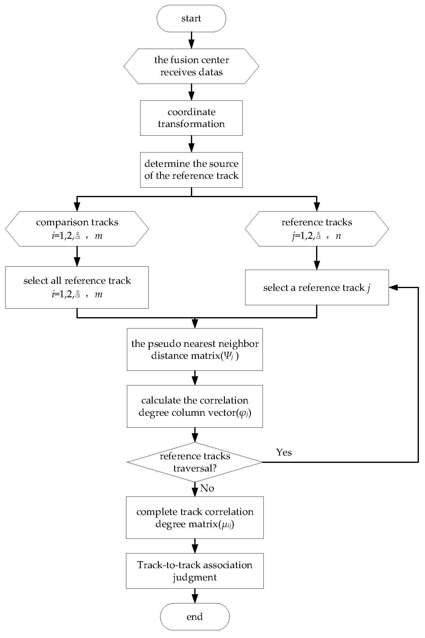
• By defining the pseudo nearest neighbor distance between the coordinate points of the track and the track data set, the correlation degree between the tracks is established, and an asynchronous TTTA algorithm based on pseudo nearest neighbor distance is proposed. This algorithm does not need time domain alignment, reduces steps, effectively avoids introducing estimation bias, and directly associates the track data.
• The average correct association rate of the tracks of the algorithm under different cycle ratios, different delay startup times, and different noise distribution forms is analyzed, and the anti-interference and effectiveness of the algorithm are proved.
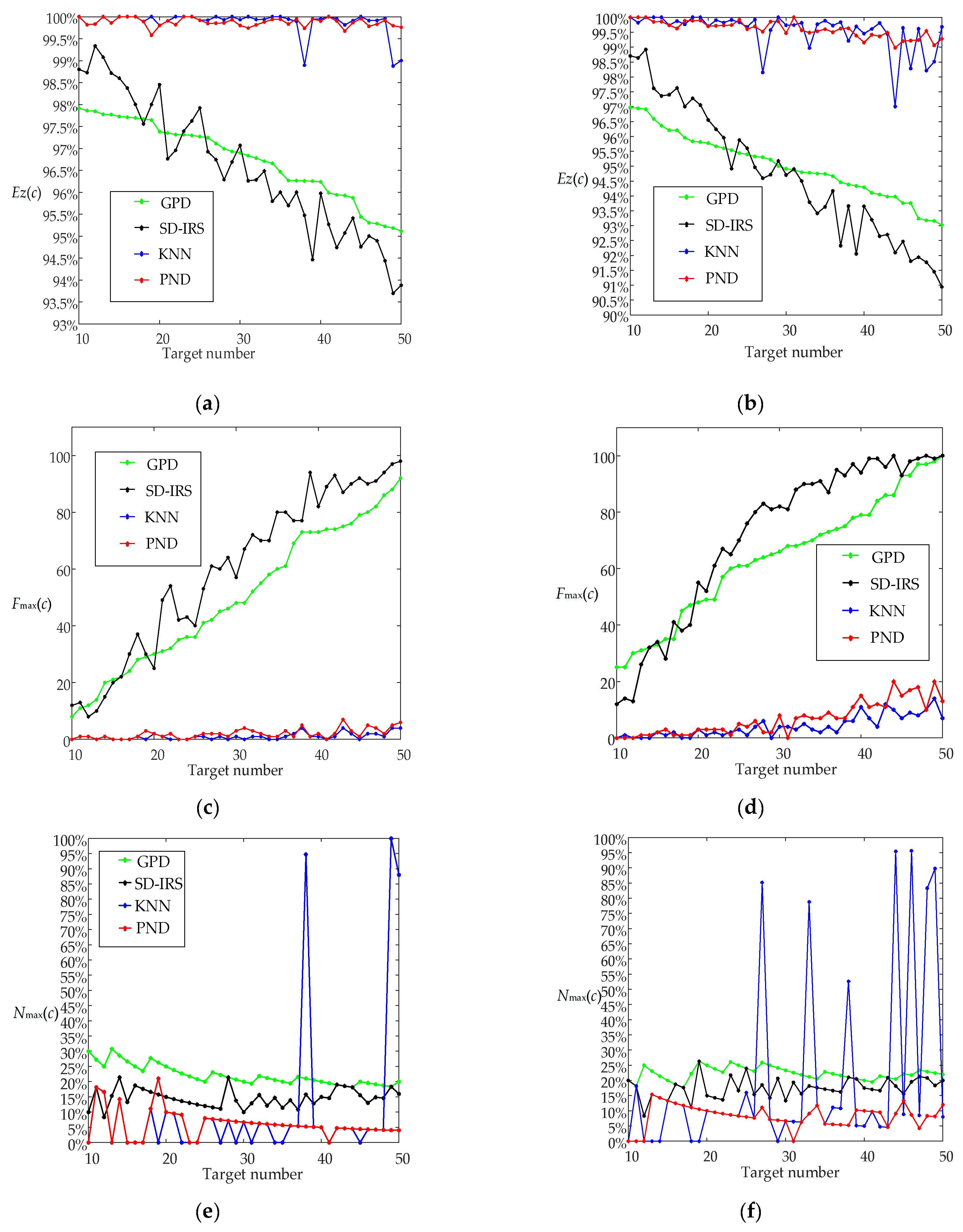
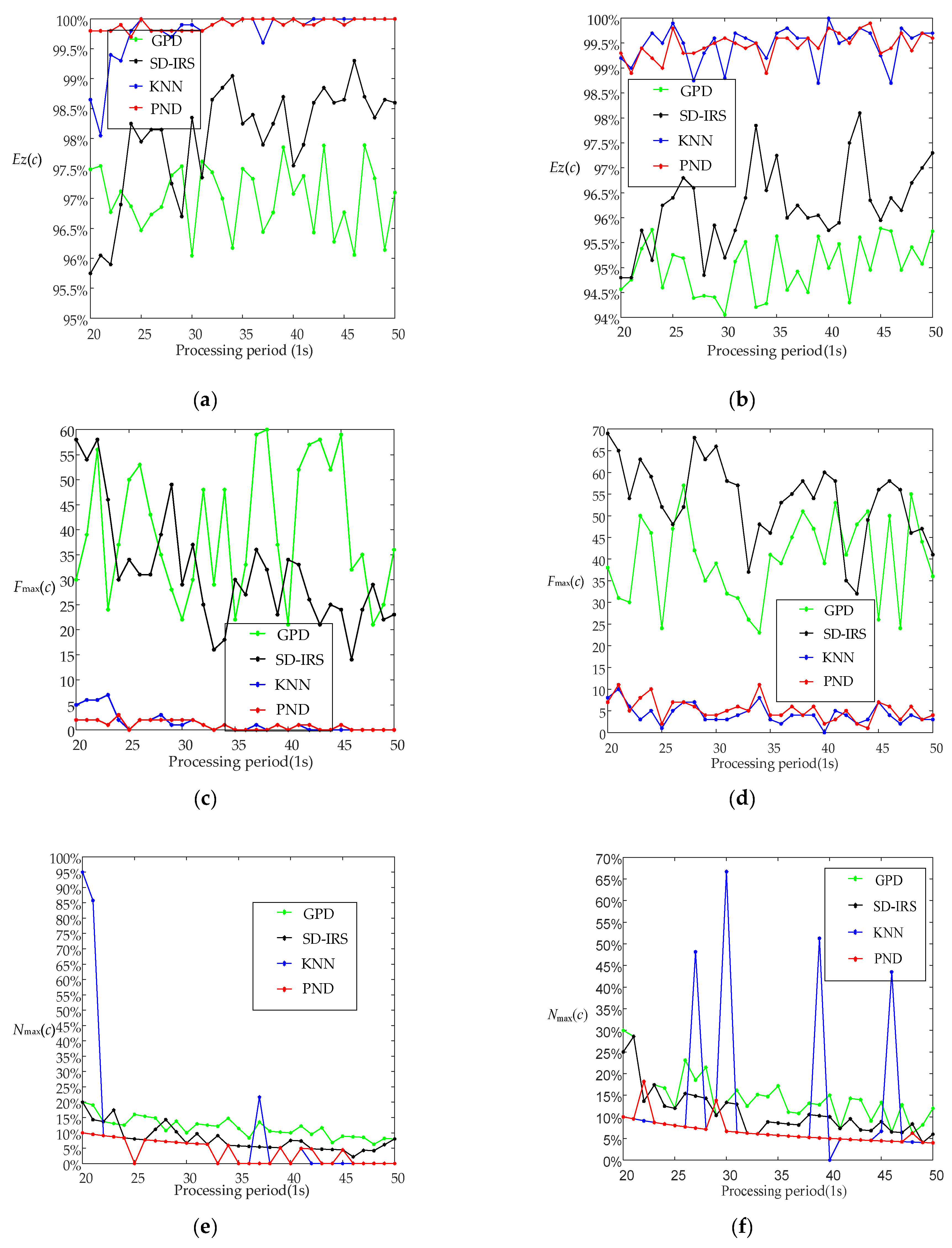
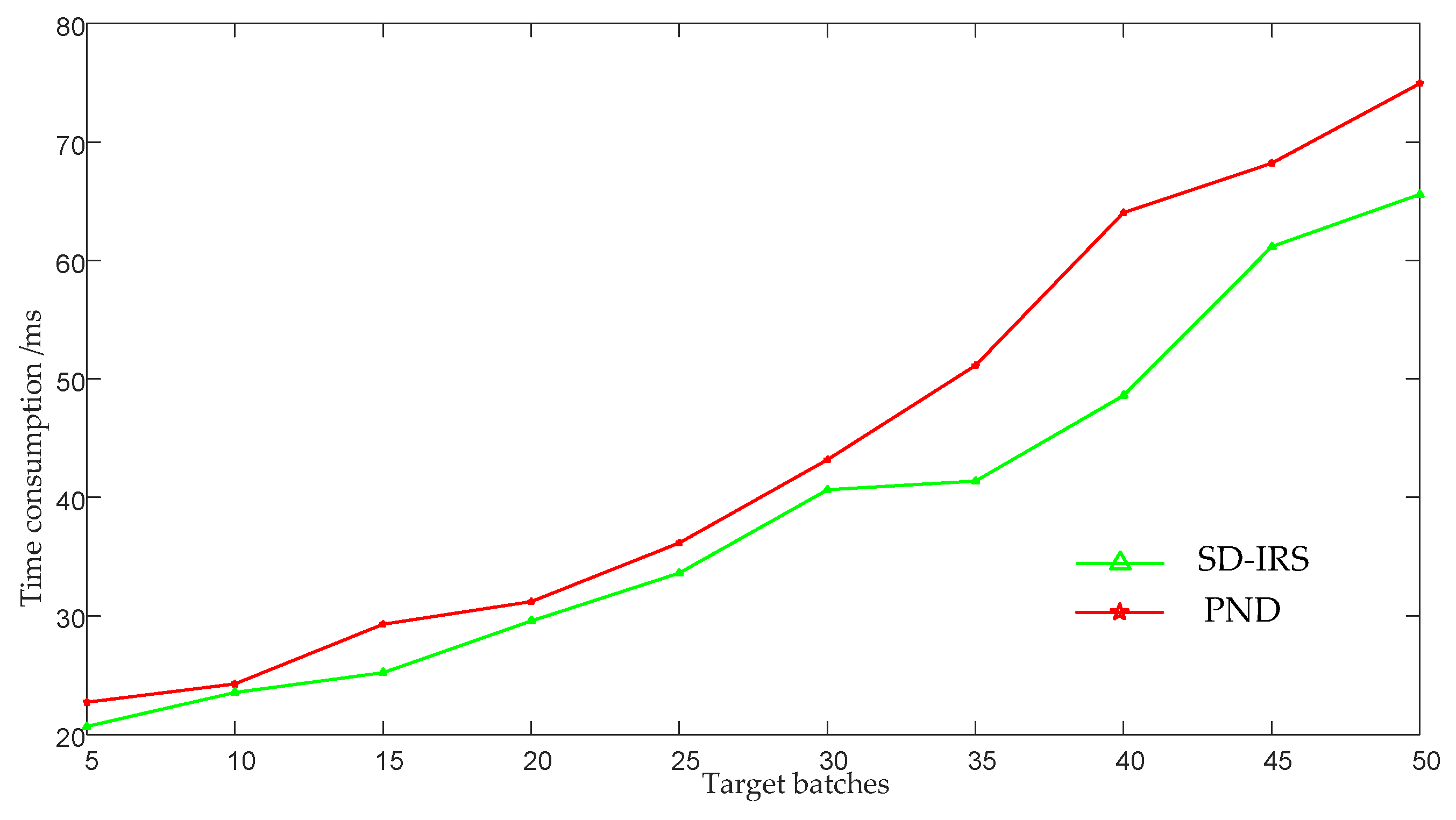
• In different targets’ moving environments, by changing the simulation conditions of the number of target batches and processing periods, the number of false associations, the maximum false association rates, and the average correct association rate of various algorithms are compared, which proves that the proposed algorithm has strong robustness and superiority.

The main innovation of this paper is to derive and propose an asynchronous TTTA algorithm based on pseudo nearest neighbor distance. The structure of the article is as follows. Section 2 defines the pseudo nearest neighbor distance and the degree of correlation between different tracks, and the asynchronous TTTA algorithm is derived in detail. Section 3 carries out simulation experiments and analyzes the results according to performance evaluation indicators. Finally, Section 4 provides conclusions.

2. Materials and Methods

2.1. Mathematical Formula Definition

Definition 1. 

Pseudo nearest neighbor distance between track coordinate point and track data set.

Assuming that the non-empty track coordinate data set $H^i=\left\{h^i\left(1\right),h^i\left(2\right),\cdots ,h^i\left(l\right)\right\}$, $i=1,2,\cdots ,m$, in which the coordinate points $h^i\left(q\right)=\left(x^i\left(q\right),y^i\left(q\right),z^i\left(q\right)\right)\in R^3$, $q=1,2,\cdots l$, the Euclidean distance between any coordinate point of any other non-empty track $h^j\left(p\right)=\left(x^j\left(p\right),y^j\left(p\right),z^j\left(p\right)\right)\in R^3$($j=1,2,\cdots ,n$, $p=1,2,\cdots k$) and track point $h^i\left(q\right)$ is

$$\begin{array}{l}{d}_q=\Vert h^i\left(q\right),h^j\left(p\right)\Vert \\ =\sqrt{{\left(x^i\left(q\right)-x^j\left(p\right)\right)}^2+{\left(y^i\left(q\right)-y^j\left(p\right)\right)}^2+{\left(z^i\left(q\right)-z^j\left(p\right)\right)}^2}.\end{array}$$

(1)

then

$$d_{N-ij}=d\left(H^i,h^j\right)=\min \left(d_1,d_1,\cdots ,d_n\right)$$

(2)

is the pseudo nearest neighbor distance between the track coordinate data set Hⁱ and the coordinate point h^j.

Definition 2. 

Correlation degree between different tracks.

Assuming that there are coordinate data set array $H=\left\{H^1,H^2,\cdots ,H^i,\cdots ,H^m\right\}$ of m tracks and coordinate data set $H^j=\left\{h^j\left(1\right),h^j\left(2\right),\cdots ,h^j\left(p\right)\right\}$ of the jth track, and $H^j\notin H$, where $h^j\left(p\right)=\left(x^j\left(p\right),y^j\left(p\right),z^j\left(p\right)\right)\in R^3$, then the correlation degree between track coordinate data set $H^j$ and $H^i$ is defined as:

$$\phi \left(H^i,H^j\right)=\frac{1}{k}{\displaystyle \sum _{p=1}^k\eta \left(H^i,h^j\left(p\right)\right)}.$$

(3)

In the formula:

$$\eta \left(H^i,h^j\left(p\right)\right)=\frac{\underset{i}{\min }\underset{p}{\min }{d}_{ij}\left(p\right)+\delta \underset{i}{\max }\underset{p}{\max }{d}_{ij}\left(p\right)}{d_{ij}\left(p\right)+\delta \underset{i}{\max }\underset{p}{\max }{d}_{ij}\left(p\right)}.$$

(4)

Indicates the grey correlation coefficient of track coordinate data set $H^j$ and $H^i$ [30]. The real number represents the resolution coefficient, which is generally 0.5, and $d_{ij}\left(p\right)=d_{N-ij}\left(p\right)=d\left(H^i,h^j\left(p\right)\right)$.

2.2. Asynchronous Track-to-Track Association Algorithm Based on Pseudo Nearest Neighbor Distance

This article takes two radars, R₁ and R₂, as examples. The process of an asynchronous unequal rate TTTA algorithm is shown in Figure 1.

The two radars R₁ and R₂ search and track multiple batches of targets within the detection range, and the output track serial number sets are $T_{R_1}=\left\{1,2,\cdots ,m\right\}$ and $T_{R_2}=\left\{1,2,\cdots ,n\right\}$, respectively. In addition, due to the differences in radar detection range, startup time and search frequency, the number of tracks in sets $T_{R_1}$ and $T_{R_2}$ is not equal, that is, $m\ne n$. Then the correlation degree formula ${\phi }_{ij}=\phi \left(H_{R_1}^i,H_{R_2}^j\right)$ between different tracks of two radars can be expressed as

$${\widehat{\phi }}_{ij}=\phi \left({\widehat{H}}_{R_1}^i,{\widehat{H}}_{R_2}^j\right).$$

(5)

In the formula: $H_{R_1}^i$ and $H_{R_2}^j$ represent the true state vector data set of the ith track of radar R₁ and the jth track of radar R₂, respectively; ${\widehat{H}}_{R_1}^i$ and ${\widehat{H}}_{R_2}^j$ represent the state estimation vector data set of the ith track of radar R₁ and the jth track of radar R₂, respectively.

Firstly, the track data is converted to the FC through coordinates, and the track of the radar is selected as the reference track according to the sampling rate of the two radars, so as to calculate the pseudo nearest neighbor distance between the jth reference track and all the comparison tracks according to definition 1. Then, according to definition 2, the correlation degree ${\phi }_j$ between the jth reference track and all the comparison tracks is obtained. By analogy, the correlation degree between other reference tracks and all the comparison tracks is calculated, and the correlation degree matrix ${\phi }_{ij}$ of all the tracks of the two radars is established. ${\phi }_{ij}$ reflects the degree of correlation between tracks. The higher the value, the greater the probability that two tracks are the same target. Finally, the corresponding objective function is established according to the correlation degree matrix, and the Jonker-Volgenant algorithm and the classical allocation method are combined to traverse the global tracks assignment to obtain the optimal solution.

The following is a detailed derivation of the asynchronous unequal rate TTTA algorithm calculation process using two three-coordinate radars as examples, which can be calculated by analogy for multiple radars.

2.2.1. Data Reception

Assuming that the two radars are asynchronous and have different scanning periods, T is the data processing period of the fusion center. Taking the c processing period ($\left[\left(c-1\right)T,T\right]$) as an example, the number of track batches reported by radar R₁ and R₂ are m and n respectively, then the reported track coordinate data sets $A_{R_1}\left(c\right)$ and $A_{R_2}\left(c\right)$ can be expressed as

$$A_{R_1}\left(c\right)=\left\{A_{R_1}^1\left(c\right),A_{R_1}^2\left(c\right),\cdots ,A_{R_1}^i\left(c\right),\cdots ,A_{R_1}^m\left(c\right)\right\},$$

(6)

$$A_{R_2}\left(c\right)=\left\{A_{R_2}^1\left(c\right),A_{R_2}^2\left(c\right),\cdots ,A_{R_2}^j\left(c\right),\cdots ,A_{R_2}^n\left(c\right)\right\}.$$

(7)

In the formula, $A_{R_1}^i\left(c\right)$ and $A_{R_2}^j\left(c\right)$, respectively, represent the ith and jth track data of radar R₁ and R₂ within the c processing period.

Considering that the radar network system has leakage points due to transmission channel damage in practice, the number of track points reported by the radar may not be equal. If the ith track of radar R₁ contains $n_{R_1}^i$ track points, the coordinate data set of the ith track is

$${\widehat{A}}_{R_1}^i\left(c\right)=\left\{{\widehat{X}}_{R_1}^i\left(t_{R_1}^1\right),{\widehat{X}}_{R_1}^i\left(t_{R_1}^2\right),\cdots ,{\widehat{X}}_{R_1}^i\left(t_{R_1}^{n_{R_1}^i}\right)\right\}$$

(8)

In the formula, ${\widehat{X}}_{R_1}^i\left(t_{R_1}^e\right)$ represents the polar coordinate state estimate of the eth track point of the ith track reported by radar R₁ for the cth processing period; $t_{R_1}^e$ represents the time stamp of the corresponding track point.

Similarly, the coordinate data set of the jth track of radar R₂ containing $n_{R_2}^j$ track points can be expressed as

$${\widehat{A}}_{R_2}^j\left(c\right)=\left\{{\widehat{X}}_{R_2}^j\left(t_{R_2}^1\right),{\widehat{X}}_{R_2}^j\left(t_{R_2}^2\right),\cdots ,{\widehat{X}}_{R_2}^j\left(t_{R_2}^{n_{R_2}^j}\right)\right\}$$

(9)

The track points $\widehat{X}$ in the track data set reported by the radar include slope range r, azimuth Angle θ, and pitch Angle β.

2.2.2. Coordinate Transformation

The track point reported by the radar is the estimated value of the polar coordinate state $\left(\widehat{r},\widehat{\theta },\widehat{\beta }\right)$. Due to the fact that stations in the radar network system are not at the same point and are relatively distant from each other, considering the influence of the curvature of the Earth, the radar station and the fusion center are not on the same plane, as shown in Figure 2.

If we simply establish their respective rectangular coordinate systems for coordinate transformation, coordinate transformation error will be introduced to affect the TTTA. Therefore, it is necessary to take the FC station center rectangular coordinate system as the unified coordinate system for data processing under the Earth-Centered Earth-Fixed (ECEF) coordinate system, and convert the data reported by the radar into geographical coordinates [31] to obtain the rectangular coordinates of the track point $\left(\widehat{x},\widehat{y},\widehat{z}\right)$. Then, the ith track coordinate data set of radar R₁ in the cth processing period can be obtained:

$${\widehat{H}}_{R_1}^i\left(c\right)=\left\{{\widehat{h}}_{R_1}^i\left(1\right),{\widehat{h}}_{R_1}^i\left(2\right),\cdots ,{\widehat{h}}_{R_1}^i\left(n_{R_1}^i\right)\right\}.$$

(10)

In the formula, ${\widehat{h}}_{{}_{R_1}}^i\left(q\right)=\left({\widehat{x}}_{{}_{R_1}}^i\left(q\right),{\widehat{y}}_{{}_{R_1}}^i\left(q\right),{\widehat{z}}_{{}_{R_1}}^i\left(q\right)\right)\in R^3$ represents the three-dimensional coordinate of the qth track point in the coordinate data set of the ith track of radar R₁ for the cth processing period, $q=1,2,\cdots ,n_{R_1}^i$.

Similarly, the jth track coordinate data set of radar R₂ in the cth processing period can be obtained:

$${\widehat{H}}_{R_2}^j\left(c\right)=\left\{{\widehat{h}}_{R_2}^j\left(1\right),{\widehat{h}}_{R_2}^j\left(2\right),\cdots ,{\widehat{h}}_{R_2}^j\left(n_{R_2}^j\right)\right\}.$$

(11)

2.2.3. Reference Track Selection

Because the radar is asynchronous and the sampling rate is generally not equal, selecting the appropriate reference track can reduce the introduction of biases in calculating the pseudo nearest neighbor distance that can represent the distance between two tracks. As shown in Figure 3, assuming that two tracks are from the same target of different radars, the sampling rate of radar R1 is less than that of radar R2, and the startup time is inconsistent. Due to the existence of biases, the tracks do not coincide.

It can be seen from the figure that the track points of radar R₁ and R₂ are distributed in disorder. In time t₂, when track i is selected as the reference track, the pseudo nearest neighbor distance is only one (l₁). While track j is selected as the reference track, there are two pseudo nearest neighbor distances (l₂, l₃). Obviously, the minimum l₁ is closer to the real distance between the two tracks, and the information is more representative. Moreover, there are biases between the pseudo nearest neighbor distance and the real distance. The number of the pseudo nearest neighbor distance obtained by taking track j as the reference track is significantly more than track i, which will increase the calculation biases. Therefore, the track reported from the radar with the lower sampling rate is selected as the reference track before calculating the track correlation degree.

2.2.4. Derivation of Track Correlation Matrix

Assuming that the reference track is from radar R₂, according to the definition of pseudo nearest neighbor distance between the coordinate point and the track coordinate data set in definition 1, the pseudo nearest neighbor distance matrix between all the comparison tracks and the jth reference track in the c processing period is calculated as:

$${\Psi }_j\left(c\right)={\left[d_{i,q}\right]}_{m\times n_{R_2}^j}=\left[\begin{array}{cccc}{d}_{1,1}& d_{1,2}& \cdots & d_{1,n_{R_2}^j}\\ d_{2,1}& d_{2,2}& \cdots & d_{2,n_{R_2}^j}\\ ⋮& ⋮& & ⋮\\ d_{m,1}& d_{m,2}& \cdots & d_{m,n_{R_2}^j}\end{array}\right].$$

(12)

In the formula:

$$d_{i,p}=d\left({\widehat{H}}_{R_1}^i\left(c\right),{\widehat{h}}_{R_2}^j\left(p\right)\right),{\widehat{h}}_{R_2}^j\left(p\right)\in {\widehat{H}}_{R_2}^j\left(c\right).$$

(13)

Then according to Definition 2, the correlation degree column vector of the jth track of radar R₂ and all tracks of radar R₁ can be obtained as:

$${\phi }_j\left(c\right)={\left[{\widehat{\phi }}_{ij}\left(c\right)\right]}_{m\times 1}={\left[\phi \left({\widehat{H}}_{R_1}^i\left(c\right),{\widehat{H}}_{R_2}^j\left(c\right)\right)\right]}_{m\times 1.}$$

(14)

In the formula:

$$\phi \left({\widehat{H}}_{R_1}^i\left(c\right),{\widehat{H}}_{R_2}^j\left(c\right)\right)=\frac{1}{k}{\displaystyle \sum _{p=1}^k\eta \left({\widehat{H}}_{R_1}^i\left(c\right),{\widehat{h}}_{R_2}^j\left(p\right)\right),}$$

(15)

$$\eta \left({\widehat{H}}_{R_1}^i\left(c\right),{\widehat{h}}_{R_2}^j\left(p\right)\right)=\frac{\underset{i}{\min }\underset{p}{\min }{d}_{i,p}+\delta \underset{i}{\max }\underset{p}{\max }{d}_{i,p}}{d_{i,p}+\delta \underset{i}{\max }\underset{p}{\max }{d}_{i,p}}.$$

(16)

By analogy, the correlation degree column vector of all tracks of radar R₂ and all tracks of radar R₁ is obtained. Finally, the correlation degree matrix of tracks is:

$${\phi }_{ij}\left(c\right)={\left[{\phi }_1\left(c\right),{\phi }_2\left(c\right),\cdots ,{\phi }_n\left(c\right)\right]}_{m\times n}$$

(17)

2.2.5. Track-to-Track Association Judgment

The $m\times n$ dimensional asynchronous track correlation degree matrix ${\phi }_{ij}\left(c\right)$ of formula (17) is obtained from the previous article, and $m\ne n$. Considering the problem of tracks missing due to transmission channel damage and completing all tracks association, expand ${\phi }_{ij}\left(c\right)$ into a square matrix, take ${\rm M}=\max \left(m,n\right)$, and use 0 to complete ${\phi }_{ij}\left(c\right)$ into an M-order square matrix ${\mu }_{ij}\left(c\right)$, and the supplemented elements are considered as virtual targets. Then, the Jonker-Volgenant algorithm and the classical allocation method are combined to perform the correlation judgment on the tracks.

Setting:

$${\delta }_{ij}=\{\begin{array}{l}1\begin{array}{ccc}& & \mathrm{Indicates} \mathrm{that} \mathrm{the} i\mathrm{th} \mathrm{track} \mathrm{and} \mathrm{the} j\mathrm{th} \mathrm{track} \mathrm{are} \mathrm{the} \mathrm{same} \mathrm{target}\end{array}\hfill \\ 0\begin{array}{ccc}& & \mathrm{Indicates} \mathrm{that} \mathrm{the} i\mathrm{th} \mathrm{track} \mathrm{and} \mathrm{the} j\mathrm{th} \mathrm{track} \mathrm{are} \mathrm{not} \mathrm{the} \mathrm{same} \mathrm{target}\end{array}\hfill \end{array}$$

(18)

The objective function is marked as:

$$L\left(c\right)={\displaystyle \sum _{i=1}^M{\displaystyle \sum _{j=1}^M{\delta }_{ij}\cdot }}{\mu }_{ij}\left(c\right).$$

(19)

Since the greater the correlation degree between tracks means the greater the probability of tracks being the same target, the objective function in (19) can be converted into the following two-dimensional allocation problem:

$$\{\begin{array}{c}\underset{{\delta }_{ij}}{\min }{\displaystyle \sum _{i=1}^M{\displaystyle \sum _{j=1}^M{\delta }_{ij}\cdot \left(1-{\mu }_{ij}\left(c\right)\right)}}\\ {\displaystyle \sum _{i=1}^M{\delta }_{ij}=1,\forall j\in \left\{1,2,\cdots ,M\right\}}\\ {\displaystyle \sum _{j=1}^M{\delta }_{ij}=1,\forall i\in \left\{1,2,\cdots ,M\right\}}\end{array}.$$

(20)

Then the Jonker-Volgenant algorithm is used to minimize the value of the objective function, and the correlation degree matrix between tracks can be solved. Among them, the Jonker-Volgenant algorithm is much faster than the famous Hungarian algorithm. The complexity of this algorithm is low, and its computational complexity is O(N³). The specific steps will not be repeated here.

3. Experiments and Performance Analysis

3.1. Simulation Environment and Evaluation Index

The simulation environment is the Windows 10 64-bit operating system and Matlab R2021a software platform. The main parameters of the computer used in the simulation are as follows: the processor is Intel Core i5-11400 H, the main frequency is 2.70 GHz, and the memory is 16.0 GB.

It is assumed that there are two 3D coordinate radars in the distributed radar network system to search and track targets in the public area, and the radar has no missing or wrong information in the target search. The simulation scenario parameters are shown in

Table 1. Simulation scene parameters.

Parameter Settings	Geographical Coordinates	Slope Range System Error	Azimuth Angle System Error	Pitch Angle System Error
R1	(0°, 0°, 0 m)	150 m	0.01 rad	0.02 rad
R2	(0°, 0.2°, 0 m)	100 m	0.01 rad	0.01 rad

.

In order to ensure the reliability and superiority of the experimental results, each group of data was subjected to $W=100$ Monte Carlo experiments. The number of false associations $F_{\max }\left(c\right)$, the maximum false association rate $N_{\max }\left(c\right)$, and the average correct association rate $Ez\left(c\right)$ were used as the evaluation indexes of the TTTA effect. $F_{\max }\left(c\right)$ is defined as the number of experiments with track false association in $W$ times Monte Carlo experiments. $N_{\max }\left(c\right)$ is defined as the maximum false association rate when the false association occurs in $W$ times Monte Carlo experiments. $Ez\left(c\right)$ is defined as follows:

$$Ez\left(c\right)=\frac{{\displaystyle \sum _{n=1}^W{Z}_n\left(c\right)}}{WL}\times 100\%.$$

(21)

In the formula: $Z_n\left(c\right)$ is the number of tracks correctly associated by the FC in the nth experiment within the c processing period. L is the total number of target tracks in the common observation area.

3.2. Algorithm Performance Analysis

In order to prove the feasibility and superiority of the algorithm (it is called PND) designed in this paper, simulation comparison experiments were conducted by changing the simulation scene conditions and comparing with GPD [20], SD-IRS [28], and KNN [32] algorithms.

3.2.1. Algorithm Effectiveness Analysis

The parameter settings for simulation scenario 1 are shown in

Table 2. The parameter settings for simulation scenario 1.

The Processing Period of the FC	The Number of Targets	The Motion Starting Direction	The Motion Starting Velocity	The Sampling Period of Radar R2
50 s	20	0~2π rad	100~300 m/s	4 s

. All the observed targets move in a straight line with approximate uniform speed.

The radar R₂ and R₁ are turned on at the same time, and k represents the ratio of the sampling period of radar R₁ to that of radar R_2.

$$k=\frac{T_{R_1}}{T_{R_2}}.$$

(22)

Table 3. Time consuming of algorithms with different values of k.

Sampling Period Ratio	k = 1	k = 1.5	k = 2	k = 2.5	k = 3
time-consuming(s)	2.4318	1.6680	1.3570	1.1446	0.9537

lists the comparison of calculation time under different period ratios. It can be seen that as the ratio increases from 1 to 3, the time consumption decreases significantly. This is because the increase of the ratio is equivalent to the decrease of the number of radar R1 track points that need to be processed, thus reducing the amount of calculation.

Table 4. The change of the false association times $F_{\max }\left(c\right)$ and the average correct association rate $Ez\left(c\right)$ with different k values and startup time difference.

Startup Time Difference(s)	The Evaluation Indexes	Sampling Period Ratio
		k = 1	k = 1.5	k = 2	k = 2.5	k = 3
1	$F_{\max }\left(c\right)$	1	1	0	1	1
	$Ez\left(c\right)$	99.9%	99.9%	100%	99.9%	99.9%
1.5	$F_{\max }\left(c\right)$	0	0	0	0	1
	$Ez\left(c\right)$	100%	100%	100%	100%	99.9%
2	$F_{\max }\left(c\right)$	0	1	0	0	0
	$Ez\left(c\right)$	100%	99.9%	100%	100%	100%
2.5	$F_{\max }\left(c\right)$	1	0	1	0	1
	$Ez\left(c\right)$	99.9%	100%	99.9%	100%	99.9%

lists the false association times $F_{\max }\left(c\right)$ and the average correct association rate $Ez\left(c\right)$ under different period ratios and startup times. It can be seen that the average correct association rate is 99.9%~100%, and the maximum track false association occurs only once. The high correlation rate indicates that the startup time and radar sampling rate have no special impact on the correct association rate of the algorithm. This is because different sampling rates only affect the number of track points. However, the center of gravity of the algorithm in this paper is to calculate the pseudo nearest neighbor distance between each point of all comparison tracks and the reference track point, and there is no requirement for the track length. In essence, the time difference of radar startup also makes the time of track points different. However, the algorithm in this paper does not require time parameters to solve the pseudo nearest neighbor distance between tracks, so it has no significant impact on the final settlement result. The effectiveness of the algorithm is proved.

Table 5. Average correct association rate $Ez\left(c\right)$ of different noise distributions.

Different Noise Distribution Forms	Gaussian Distribution	Rayleigh Distribution	Exponential Distribution	Uniform Distribution
$Ez\left(c\right)$	99%	100%	99%	100%

shows the average correct association rate of the algorithm in different noise distribution forms. It can be seen from the data in the table that the algorithm in this paper can maintain a high average correct association rate under the four noise distribution forms of Gaussian, Rayleigh, Exponential, and Uniform, and is less affected by the noise distribution forms, which proves that the algorithm has strong anti-noise performance.

3.2.2. Analysis of Different Target Numbers and Different Movement Forms

The parameter settings for simulation scenario 2 are shown in

Table 6. The parameter settings for simulation scenario 2.

The Processing Period of the FC	The Motion Starting Direction	The Motion Starting Velocity	The Maneuvering Turning Rate	The Sampling Period of Radar R1	The Sampling Period of Radar R2	The Number of Targets
30 s	0~2π rad	100~300 m/s	0.05~0.5	4 s	5 s	10:1:50

. The target is simulated under two conditions of uniform linear motion and uniform turning motion.

Figure 4 shows the comparison of the false association numbers $F_{\max }\left(c\right)$, the maximum false association rate $N_{\max }\left(c\right)$, and the average correct association rate $Ez\left(c\right)$ of the four algorithms under different target numbers and different movement forms. It can be seen from Figure 4 that the GPD algorithm carries out TTTA under the premise of time domain alignment, and more parameters need to be predicted. The accumulation and propagation of systematic biases lead to a low average correct association rate. With the increase of the number of targets, the association accuracy decreases, and the probability of wrong association increases. Although the SD-IRS algorithm does not make time domain alignment and directly establish correlation degree matrix for association, the accuracy of track calculation is reduced because the real sequence is transformed into a mixed sequence of interval numbers and real numbers, which affects the average correct association rate of TTTA and decreases with the increase of the number of targets. When the target made a constant turning motion, the GPD and SD-IRS algorithms were greatly affected, the average correct association rate decreased by 2%, and the false association numbers in the experiment increased significantly. The average correct association rate of KNN and PND algorithms is above 99%, and the target number has little influence on it. However, it can be seen from the comparison chart of maximum false association rate that the KNN algorithm will jump in the case of an uncertain target distribution. The number of jumps especially increases in the case of turning targets, and the maximum false association rate reaches 95%, indicating poor algorithm stability. In this paper, the PND algorithm directly uses the shortest Euclidean distance as a metric, which reduces the calculation amount and is closer to the actual nearest neighbor distance, and there is no time domain alignment bias accumulation and propagation. The average correct association rate for different types of targets is kept above 99%, the number of false associations and the maximum false association rate is low, and the algorithm is robust.

3.2.3. Analysis of Different Processing Periods and Different Movement Forms

The parameter settings for simulation scenario 3 are shown in

Table 7. The parameter settings for simulation scenario 3.

The Processing Period of the FC	The Motion Starting Direction	The motion starting velocity	The Maneuvering Turning Rate	The Sampling Period of Radar R1	The Sampling Period of Radar R2	The Number of Targets
20:2:50 s	0~2π rad	100~300 m/s	0.05~0.5	4 s	5 s	20

. The target is simulated under two conditions of uniform linear motion and uniform turning motion.

Figure 5 shows the comparison of the false association numbers $F_{\max }\left(c\right)$, the maximum false association rate $N_{\max }\left(c\right)$, and the average correct association rate $Ez\left(c\right)$ of the four algorithms under different processing periods and different movement forms. The uniform turning targets have different degrees of influence on each algorithm, while the effect of the processing period is small. From the perspective of the average correct association rate and the false association numbers, GPD and SD-IRS algorithms decreased by about 3% and increased by about 10 times, respectively, while KNN and PND algorithms decreased by about 1% and increased by about 5 times, respectively. From the perspective of the maximum false association rate, GPD and SD-IRS algorithms are significantly higher than PND algorithm in this paper. Similarly, when KNN algorithm changes drastically under certain uncertain target distribution, the PND algorithm still maintains a stable low maximum false association rate.

Table 8. Maximum false correlation rate under different target numbers in Scenario 2.

Target Number	11	12	13	14	15	16	17	18	19	20
KNN	18.18%	0.00%	0.00%	0.00%	13.33%	12.50%	11.76%	0.00%	0.00%	10.00%
PND	0.00%	0.00%	15.38%	14.29%	13.33%	12.50%	11.76%	11.11%	10.53%	10.00%
Target number	21	22	23	24	25	26	27	28	29	30
KNN	9.52%	9.09%	8.70%	8.33%	16.00%	7.69%	85.19%	7.14%	0.00%	6.67%
PND	9.52%	9.09%	8.70%	8.33%	8.00%	7.69%	11.11%	7.14%	6.90%	6.67%
Target number	31	32	33	34	35	36	37	38	39	40
KNN	6.45%	6.25%	78.79%	11.76%	5.71%	11.11%	10.81%	52.63%	5.13%	5.00%
PND	0.00%	6.25%	9.09%	11.76%	5.71%	5.56%	5.41%	5.26%	10.26%	10.00%
Target number	41	42	43	44	45	46	47	48	49	50
KNN	9.76%	4.76%	4.65%	95.45%	8.89%	95.65%	8.51%	83.33%	89.80%	8.00%
PND	9.76%	9.52%	4.65%	9.09%	13.33%	8.70%	4.26%	8.33%	8.16%	12.00%

and

Table 9. Maximum false correlation rate under different processing periods in Scenario 3.

Processing Period/S	21	22	23	24	25	26	27	28	29	30
KNN	9.52%	9.09%	8.70%	8.33%	8.00%	7.69%	48.15%	7.14%	13.79%	66.67%
PND	9.52%	18.18%	8.70%	8.33%	8.00%	7.69%	7.41%	7.14%	13.79%	6.67%
Processing period/S	31	32	33	34	35	36	37	38	39	40
KNN	6.45%	6.25%	6.06%	5.88%	5.71%	5.56%	5.41%	5.26%	51.28%	0.00%
PND	6.45%	6.25%	6.06%	5.88%	5.71%	5.56%	5.41%	5.26%	5.13%	5.00%
Processing period/S	41	42	43	44	45	46	47	48	49	50
KNN	4.88%	4.76%	4.65%	4.55%	6.67%	43.48%	4.26%	4.17%	4.08%	4.00%
PND	4.88%	4.76%	4.65%	4.55%	4.44%	4.35%	4.26%	6.25%	4.08%	4.00%

list the maximum false association rate changes for the KNN algorithm and PND algorithm for turning targets under two simulation scenarios. From the tables, it can be seen that the KNN algorithm has serious false association situations, with the maximum false association rates reaching 95.65% when the target changes and 66.67% when the processing cycle changes. The algorithm in this paper is only 15.38% and 18.18%, respectively. It is proved that the algorithm in this paper has strong robustness and advantages, and also shows that the algorithm in this paper has high accuracy.

3.2.4. Algorithm Complexity Analysis

On the premise that the two radars have the same sampling rate,

Table 10. Algorithm computation volume comparison.

Algorithm Type	SD-IRS	PND
Multiplication operation amount	2 mn2 + mn	6 mn2 + mn
Amount of addition operations	4 mn2 − mn	6 mn2 − mn

compares the multiplication and addition amounts of the SD-IRS algorithm and the PND algorithm in this paper, where m is the number of target batches and n is the number of track points. Obviously, the computational complexity of the algorithm in this paper is higher than that of the SD-IRS algorithm.

Figure 6 compares the time consumption of the two algorithms under different target batches. It can be seen that as the number of target batches increases, the proposed algorithm takes longer than SD-IRS algorithm, and the results are consistent with the theoretical analysis in Table 10.

4. Conclusions

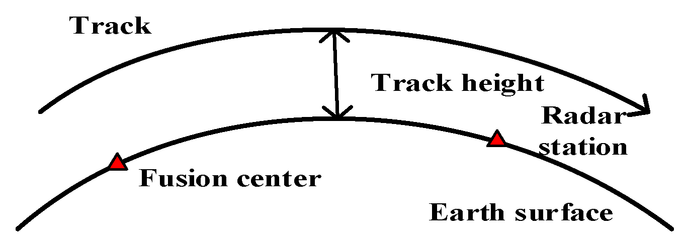
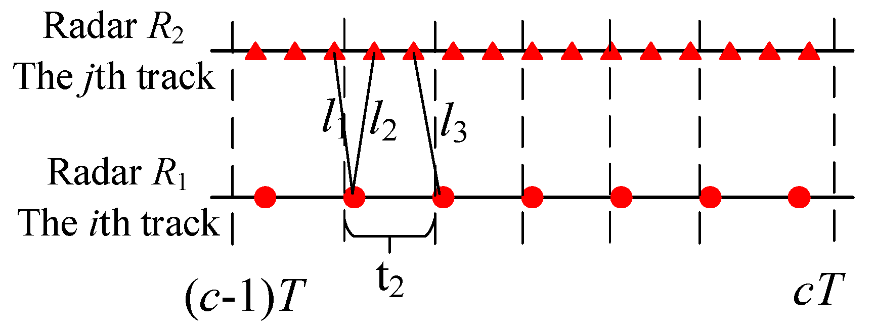
In order to solve the problem of TTTA in the case of asynchronous unequal rates, this paper presents a rule for measuring the correlation degree between unequal length track data sets. The shortest Euclidean distance between track data sets and track points is used instead of the traditional calculation of the nearest neighbor distance between two track points at the same time. Additionally, the pseudo nearest neighbor distance between targets is directly calculated, and the correlation degree matrix between tracks is calculated using gray correlation theory, which reduces the computation amount and effectively avoids the estimation biases introduced by the time domain alignment. It has a high average correct association rate.

The algorithm does not need time domain alignment, and directly correlates the reported asynchronous unequal rate tracks. It can effectively solve the difficulty of TTTA caused by different sampling periods and inconsistent startup times of networked radars, and is not affected by processing periods and noise distribution forms. It also maintains a low and stable number of false associations, the maximum false association rate, and a high average correct association rate under different moving forms of targets, with good anti-noise, superiority, and robustness.

References

1. Durr, A.; Schweizer, B.; Bechter, J.; Waldschmidt, C. Phase noise mitigation for multistatic FMCW radar sensor networks using carrier transmission. IEEE Microw. Wirel. Compon. Lett. 2018, 28, 1143–1145. [Google Scholar] [CrossRef] [Green Version]
2. Ren, P.; Munari, A.; Petrova, M. Performance tradeoffs of joint radar-communication networks. IEEE Wirel. Commun. Lett. 2018, 8, 165–168. [Google Scholar] [CrossRef] [Green Version]
3. Nazari, M.; Pashazadeh, S.; Mohammad-Khanli, L. An adaptive density-based fuzzy clustering track association for distributed tracking system. IEEE Access 2019, 7, 135972–135981. [Google Scholar] [CrossRef]
4. Yang, D.; Ji, H.; Gao, Y. A robust D-S fusion algorithm for multi-target multi-sensor with higher reliability. Inf. Fusion 2019, 47, 47. [Google Scholar]
5. He, X.; Wang, T.; Liu, W.; Luo, T. Measurement data fusion based on optimized weighted least-squares algorithm for multi-target tracking. IEEE Access 2019, 7, 13901–13916. [Google Scholar] [CrossRef]
6. Chen, B.; Zhang, W.A.; Yu, L.; Hu, G.; Song, H. Distributed fusion estimation with communication bandwidth constraints. IEEE Trans. Autom. Control 2015, 60, 1398–1403. [Google Scholar] [CrossRef]
7. Okello, N.N.; Challa, S. Joint sensor registration and track-to-track fusion for distributed trackers. IEEE Trans. Aerosp. Electron. Syst. 2004, 40, 808–823. [Google Scholar] [CrossRef]
8. Xu, L.; Jin, S.L.; Yin, G.S. A track association algorithm based on leader-follower on-line clustering in dense target environment. Radioengineering 2014, 23, 259–265. [Google Scholar]
9. Zhu, H.; Wang, W.; Wang, C. Robust track-to-track association in the presence of sensor biases and missed detections. Inf. Fusion 2016, 27, 33–40. [Google Scholar] [CrossRef]
10. Wang, X.; Xu, Z.; Gou, X. Consensus-based track association with multistatic sensors under a nested probabilistic-numerical linguistic environment. Sensors 2019, 19, 1381–1389. [Google Scholar] [CrossRef] [Green Version]
11. Yu, Y.; Hou, Q.; Zhang, W.; Zhang, J. A sequential two-stage track-to-track association method in asynchronous bearings-only sensor networks for aerial targets surveillance. Sensors 2019, 19, 3175–3193. [Google Scholar] [CrossRef] [PubMed] [Green Version]
12. Lian, F.; Hou, L.; Wei, B.; Han, C. Sensor selection for decentralized large-scale multi-target tracking network. Sensors 2018, 18, 4115–4123. [Google Scholar] [CrossRef] [PubMed] [Green Version]
13. Kanyuck, A.J.; Singer, R.A. Correlation of multiple-site track data. IEEE Trans. Aerosp. Electron. Syst. 1970, 6, 180–187. [Google Scholar] [CrossRef]
14. Jian, G.; You, H.; Ying-Ning, P. Distributed CFAR detector based on local test statistic. Signal Process. 2000, 80, 373–379. [Google Scholar] [CrossRef]
15. Liu, Y.; Yao, L.; Xiong, W.; Zhou, Z. GF-4 Satellite and automatic identification system data fusion for ship tracking. IEEE Geosci. Remote Sens. Lett. 2019, 16, 281–285. [Google Scholar] [CrossRef]
16. Zhu, H.; Leung, H.; Yuen, K.V. A joint data association, registration, and fusion approach for distributed tracking. Inf. Sci. 2015, 324, 186–196. [Google Scholar] [CrossRef]
17. Qi, L.; Dong, K.; Liu, Y. Anti-bias track-to-track association algorithm based on distance detection. IET Radar Sonar Navigat. 2017, 11, 269–276. [Google Scholar] [CrossRef]
18. Bu, S.; Zhou, C.; Zhou, G. Simultaneous spatiotemporal bias and state estimation for asynchronous multi-sensor system. J. Eng. 2019, 19, 5824–5828. [Google Scholar] [CrossRef]
19. Tian, W.; Wang, Y.; Shan, X.; Yang, J. Track-to-track association for biased data based on the reference topology feature. IEEE Signal Process. 2014, 21, 449–453. [Google Scholar] [CrossRef]
20. Zhu, H.; Wang, M.; Yuen, K.V.; Leung, H. Track-to-track association by coherent point drift. IEEE Signal Process. 2017, 24, 643–647. [Google Scholar] [CrossRef]
21. Zheng, J.-C.; Wang, Y.; Lin, C.-C.; Zhang, X.-L.; Liu, J.; Ji, L.-W. A fusion algorithm of target dynamic information for asynchronous multi-sensors. Microsyst. Technol. 2018, 24, 3995–4005. [Google Scholar] [CrossRef]
22. Sönmez, H.H.; Hocaoğlu, A.K. Asynchronous track-to-track association algorithm based on reference topology feature. Signal Image Video Process. 2021, 16, 789–796. [Google Scholar] [CrossRef]
23. Sun, W.; Li, X.; Pang, Z.; Ji, Y.; Dai, Y.; Huang, W. Track-to-Track Association Based on Maximum Likelihood Estimation for T/R-R Composite Compact HFSWR. IEEE Trans. Geosci. Remote Sens. 2023, 61, 1–12. [Google Scholar] [CrossRef]
24. Ahmed, I.; Jun, M.; Ding, Y. A Spatio-Temporal Track Association Algorithm Based on Marine Vessel Automatic Identification System Data. IEEE Trans. Intell. Transp. Syst. 2022, 23, 20783–20797. [Google Scholar] [CrossRef]
25. Cao, Y.; Cao, J.; Zhou, Z. Track Segment Association Method Based on Bidirectional Track Prediction and Fuzzy Analysis. Aerospace 2022, 9, 274. [Google Scholar] [CrossRef]
26. Yi, X.; Zhang, H.W. A track association algorithm for distributed multi-target systems based on gray interval numbers. Acta Aeronaut. Astronaut. Sin. 2013, 34, 352–360. [Google Scholar]
27. Zu, X.; Yang, C. An EGR performance evaluation and decision-making approach based on grey theory and grey entropy analysis. PLoS ONE 2018, 13, e0191626. [Google Scholar] [CrossRef] [Green Version]
28. Yi, X.; Han, J.Y. Asynchronous track-to-track association algorithm based on similarity degree of interval-real sequence. Acta Aeronaut. Astronaut. Sin. 2015, 36, 1212–1220. [Google Scholar]
29. Yi, X.; Du, J.P. Asynchronous track-to-track association algorithm based on discrete degree of segmented sequence. Acta Aeronaut. Astronaut. Sin. 2020, 41, 265–274. [Google Scholar]
30. Xin, G.; You, H.; Xiao, Y. Gray track-to-track correlation algorithm for distributed multitarget tracking system. Signal Process. 2006, 86, 3448–3455. [Google Scholar] [CrossRef]
31. Ristic, B.; Okello, N. Sensor registration in ECEF coordinates using the MLR algorithm. In Proceedings of the 2003 Sixth International Conference of Information Fusion, Cairns, QLD, Australia, 8–11 July 2003. [Google Scholar]
32. Yi, X.; Zen, Y. Asynchronous track-to-track association algorithm based on k means distance of nearest neighbors. Syst. Eng. Electron. 2022, 44, 3515–3521. [Google Scholar]
Figure 1. Flow chart of asynchronous unequal rate TTTA algorithm.
Electronics 12 01794 g001
Figure 2. Schematic diagram of station site.
Electronics 12 01794 g002
Figure 3. Schematic diagram of asynchronous track of the same target.
Electronics 12 01794 g003
Figure 4. Scenario 2: different target numbers and different movement forms. (a) E z ( c ) comparison of different algorithms under the condition of uniform linear motion of targets; (b) E z ( c ) comparison of different algorithms in the case of target turning at constant speed; (c) F max ( c ) comparison of different algorithms under the condition of uniform linear motion of targets; (d) F max ( c ) comparison of different algorithms in the case of target turning at constant speed; (e) N max ( c ) comparison of different algorithms under the condition of uniform linear motion of targets; (f) N max ( c ) comparison of different algorithms in the case of target turning at constant speed.
Electronics 12 01794 g004
Figure 5. scenario 2: different processing periods and different movement forms. (a) E z ( c ) comparison of different algorithms under the condition of uniform linear motion of targets; (b) E z ( c ) comparison of different algorithms in the case of target turning at constant speed; (c) F max ( c ) comparison of different algorithms under the condition of uniform linear motion of targets; (d) F max ( c ) comparison of different algorithms in the case of target turning at constant speed; (e) N max ( c ) comparison of different algorithms under the condition of uniform linear motion of targets; (f) N max ( c ) comparison of different algorithms in the case of target turning at constant speed.
Electronics 12 01794 g005
Figure 6. Comparison of time consumption of different algorithms.
Electronics 12 01794 g006