Path Planning of Mecanum Wheel Chassis Based on Improved A* Algorithm

Abstract

This study is concerned with path planning in a structured greenhouse, in contrast to much of the previous research addressing applications in outdoor fields. The prototype mainly comprises an independently driven Mecanum wheel, a lidar measuring module, a single-chip microcomputer control board, and a laptop computer. Environmental information collection and mapping were completed on the basis of lidar and laptop computer connection. The path planning algorithm used in this paper expanded the 8-search-neighborhood of the traditional A* algorithm to a 48-search-neighborhood, increasing the search direction and improving the efficiency of path planning. The Floyd algorithm was integrated to smooth the planned path and reduced the turning points in the path. In this way, the problems of the traditional A* algorithm could be solved (i.e., slow the path planning speed and high numbers of redundant points). Tests showed that the turning points, planning path time, and distance of the improved algorithm were the lowest. Compared with the traditional 8-search-neighborhood A* algorithm, the turning point was reduced by 50%, the planning time was reduced by 13.53%, and the planning distance was reduced by 13.96%. Therefore, the improved method of the A* algorithm proposed in this paper improves the precision of the planning path and reduces the planning time, providing a theoretical basis for the navigation, inspection, and standardization construction of greenhouses in the future.

1. Introduction

In different agricultural applications, mobile chassis should ensure flexible movement and stable driving to improve the effectiveness and robustness of mobile chassis path planning [1,2,3]. In the existing studies, image processing technology achieves the path optimization from the perspective of obstacle detection and energy consumption reduction [4,5,6,7,8,9]. By improving the accuracy of geofencing, the optimal path selection in dynamic space can be provided [10], which can also solve problems such as vehicle collision in dynamic path planning [11] and improve the effectiveness of vehicle path planning in constrained environments [12]. Ultra-wideband positioning technology, satellite navigation technology, and multi-sensor fusion technology can also be used to complete the path planning task [13,14,15]. Path planning involves moving the chassis from the initial position to the destination position as well as planning the optimal path. The realization of path planning is a prerequisite for the application of autonomous navigation functions. Therefore, scholars worldwide have realized the application in different environments from the perspectives of communications technology, satellite navigation technology, image processing, visual recognition, SLAM (Simultaneous Localization and Mapping) technology, geo-fencing, and obstacle-avoidance processing [16,17,18,19,20,21].

The research and development of intelligent agricultural equipment, such as field picking, harvesting, transplanting, and inspection, has reduced labor costs, improved agricultural production efficiency, and opened upmarket demand—an urgent demand in the current agricultural field. In the development process of large-scale intelligent equipment, large-scale cultivation does not need to reduce the planning accuracy to a great extent, but the appearance of obstacles in the field operation process will affect the operation process and efficiency. Liu et al. [22,23] achieved the effect of obstacle avoidance by adjusting the performance of agricultural tractors and incorporating the use of a nonlinear predictive model controller. However, this method lacks flexibility for large, intelligent agricultural machines when turning on land promontories. Lu et al. [24] used the Canny algorithm to fit and synthesize polygons on the boundary lines of farmland to be harvested in the extracted satellite map and optimized the path by an arc transition algorithm, which had good obstacle avoidance and turning effect. Post et al. proposed real-time obstacle avoidance based on Hector SLAM technology with a fast and efficient planning effect [25]. In recent years, the research and development of intelligent chassis equipment in the greenhouse has also become a trend. Mahmud et al. [26] and Zangina et al. [27] marked different positions or crop positions in the moving area of the greenhouse as node information and then planned feasible paths. Too much node information in the path will lead to a long path, many turns, and lower travel efficiency. Therefore, preserving valid node information is the key to path planning [28,29]. One study found that in greenhouses with different sizes of crop areas, the running path had different widths, and its kinematic trajectory ensured the stability of the moving chassis in the narrow path [30]. However, Uyeh et al. [31] selected the most advantageous path in each seedbed to reduce the distance and time to other base points in the greenhouse. By developing standardized seedbed specifications, mobile robots can have enable fast navigation. Efficient navigation often depends on the smoothness of the path and the prior inflection principle of Liu et al. [32] and the Bezier curve principle of Zuo et al. [33], which can both improve the smoothness of the path.

The research and development of the A* algorithm [34] was proposed in 1968 on the basis of the Dijkstra algorithm [35]. Future generations of path planning research and development based on the A* algorithm are widely used in various scenarios. In the path planning of household cleaning robots, aiming at problems such as multiple search nodes and complex turning routes, the traditional A* algorithm was optimized, and the A* algorithm combined with dynamic window and pathfinding rules and algorithm structure were designed to effectively complete the path planning of household cleaning robots, but the algorithm speed needs to be improved [36,37]. In the path planning of autonomous vehicles, Bai et al. [38] proposed a motion planning algorithm based on an improved A* algorithm and a tracking control strategy based on model predictive control theory. In a study by Hong et al. [39] aiming at the long planning time of long-distance cross-country paths, the planning efficiency was improved by integrating data structures and improving retrieval strategies. Wang et al. [40] proposed an improved A* algorithm based on the heuristic function of collision cost based on the position of obstacles. Considering vehicle profile and speed, safe space is set around the vehicle to improve vehicle safety. However, the planned rate is related to the hardware conditions and the actual environment, so the actual efficiency cannot be guaranteed. Ou et al. [41] used a SLAM mapping algorithm to reduce the number of inflection points and search volume, so as to improve the stability of path search efficiency in a static environment. However, the improved algorithm has not been tested in a dynamic environment, so the accuracy and reliability of the method in a dynamic environment cannot be guaranteed. Dang et al. [42] proposed a hybrid A* algorithm based on a piecewise search to improve the safety of autonomous robots. However, due to the absence of complex smoothing technology, the computational power of this algorithm cannot handle complex environments. Farid et al. [43] proposed a 3D path planning method based on the A* algorithm to reduce nodes based on a truncation algorithm to improve the flight endurance capability of four-wing UAVs. However, other algorithms can also be further integrated to enhance the robustness of the algorithm.

This paper develops an improved path-planning algorithm based on an A* algorithm. On the basis of 2D plane mapping, firstly, the obstacles in the grid map are expanded to optimize the map environment. Then, the 8-search-neighborhood in the traditional A* algorithm is expanded to a 48-search-neighborhood in order to expand the search scope and reduce the search nodes. Moreover, the Floyd algorithm is integrated to reduce the turning points in the path and smooth the path. Finally, the simulation test of the multi-group algorithm is carried out, and the comparison test is carried out in the actual greenhouse environment. Experimental comparison and data analysis verify that the improved A* algorithm has high path planning accuracy and reduces the planning time.

2. Materials and Methods

The mobile chassis is mainly composed of the inertial navigation module, motor drive module, four independently driven Mecanum wheels, and the core controller connected with the Core I5-8300H laptop computer and equipped with Silan A1M8-R5 lidar to scan the environment and interact with the chassis controller in the ROS (Robot Operating System) of Ubuntu16.04 to complete the environment mapping and path planning. The specific hardware is shown in Figure 1.

2.1. Mobile Chassis Control System Framework Design

This study adopts the ROS system as the development platform for the control system. Path planning is accomplished through the nodes of communication between the ROS master radar and the mobile chassis. The framework of the control system is shown in Figure 2.

The basic node information, such as radar scan, chassis drive, and keyboard control, was established on the ROS development platform of the Ubuntu16.04 system. Radar and chassis control were carried out by releasing topic information through ROS master and establishing SLAM and path planning nodes to complete unfamiliar environment map construction and path planning.

In the process of moving the chassis walking, the posture of the robot body and the environment information collected by the sensor are included. The environment model is constructed in the ROS system through the complete transformation of the coordinate system. Therefore, coordinate transformation is formed through the coordinate transformation between the map, Odom, chassis center, and lidar center to complete the function of environment mapping. The origin of the map of the ROS emulator Riviz is consistent with the world coordinates. Odom represents the odometer coordinates broadcast by the chassis control function pack. Base_footprint is the projection of the center coordinate system of the moving chassis in space. And base_laser_link is a radar-centered coordinate system. The coordinates collected from base_laser_link are relative coordinates, while those collected from chassis base_link are global coordinates. Therefore, to unify the coordinates, the coordinates of base_laser_link must be converted to be consistent with those of base_link. The coordinate system is first converted from the world coordinate system to the chassis odometer coordinate system, then to the moving chassis body coordinate system, and finally to the radar coordinate system, so as to meet the requirements of the map formed by radar scanning in space.

2.2. Mecanum Wheel Chassis Motion Model

This study uses the Mecanum wheel as the moving part of the moving chassis. The motion model of the moving chassis is established after the installation mode of the Mecanum wheel is determined, and the motion mechanism of the Mecanum wheel is briefly described. Figure 3a shows a structural sketch of the moving chassis. The Mecanum wheel is composed of a wheel hub and a roller. The roller revolves around the hub and the axis of the roller is 45° to the hub axis. To ensure omnidirectional movement of the chassis, a pair of left- and right-handed Mecanum wheels are required and symmetrically mounted on the chassis.

The global cartesian coordinates are established on the chassis. The x-axis is the left and right movement direction of the chassis, and the right is positive. The y-axis is the forward and backward movement direction of the chassis, and the forward is positive. The speed of the chassis is ω, and counterclockwise is positive. The four wheat wheels are marked in order [n = 1,2,3,4], counterclockwise from the upper right corner. Assume that the speed of the chassis is $\stackrel{\rightharpoonup }{V}=\left[\begin{array}{ccc}{V}_x& V_y& \stackrel{\rightharpoonup }{\omega }\end{array}\right]$, O_n is the center point of each Mecanum wheel relative to the origin of the global coordinate O, and the coordinate is (x_n, y_n). The Mecanum wheel speed is expressed as $\stackrel{\rightharpoonup }{v_n}=\left[\begin{array}{ccc}{v}_{xn}& v_{xy}& \stackrel{\rightharpoonup }{w_n}\end{array}\right]$, and r is the radius of the Mecanum wheel. The chassis is regarded as a rigid body, and the horizontal and vertical velocity components of the chassis are equal to the horizontal and vertical components of the Mecanum-wheel center, $\stackrel{\rightharpoonup }{V}=\left[\begin{array}{cc}{V}_x& V_y\end{array}\right]$. Given that the chassis rotates at speed ω, a velocity component $\stackrel{\rightharpoonup }{v_{rn}}=\left[\begin{array}{cc}{v}_{xrn}& v_{yrn}\end{array}\right]$ (horizontal and vertical velocity components) is also generated on each wheel.

$$\{\begin{array}{c}{v}_{xn}=V_x+v_{xrn}=V_x-y_n\times w_n\\ v_{yn}=V_y+v_{yrn}=V_y+x_n\times w_n\end{array}.$$

(1)

Figure 3b shows the decomposition diagram of the velocity vector $\stackrel{\rightharpoonup }{v_n}$ of the fourth Mecanum wheel in global coordinates. $\stackrel{\rightharpoonup }{v_n}$ is the actual speed at the current moment. Figure 3b shows that $\stackrel{\rightharpoonup }{v_n}$ is synthesized by the hub center speed and center speed of the roller touching the ground. The axis of the roller is 45° to the hub axis, θ = 45°, and $w_n$ is the speed of the Mecanum wheel. Therefore, kinematics models of four Mecanum wheels can be established, as shown in Equation (2).

$$\{\begin{array}{l}{w}_{n}r=v_{xn}+v_{yn}\times tan{\theta }_n\\ \left[\begin{array}{c}{w}_1\\ w_2\\ w_3\\ w_4\end{array}\right]=\frac{1}{r}\left[\begin{array}{ccc}1& tan{\theta }_1& x_{1}tan{\theta }_1-y_1\\ 1& tan{\theta }_2& x_{2}tan{\theta }_2-y_2\\ 1& tan{\theta }_3& x_{3}tan{\theta }_3-y_3\\ 1& tan{\theta }_4& x_{4}tan{\theta }_4-y_4\end{array}\right]\left[\begin{array}{c}{V}_x\\ V_y\\ \omega \end{array}\right]\end{array}.$$

(2)

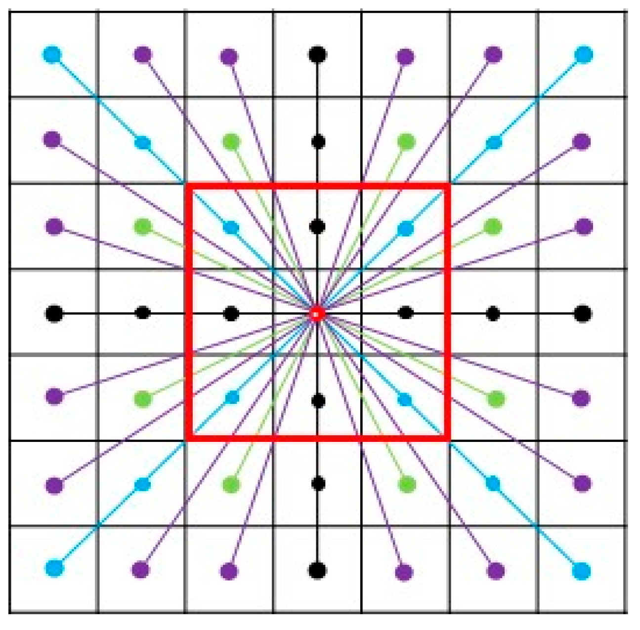
2.3. Improving the A* Algorithm

First, the map is rasterized, and the obstacle grid in the map is expanded. The 8-search-neighborhood of the A* algorithm is expanded to a 48-search-neighborhood, and the heuristic searching A* algorithm is adopted. This study refers to a cost estimation function, which is detailed with the cost relationship between the initial node, the current node, and the target node to fit an optimal path. Finally, the Floyd algorithm smooths the nodes in the fitting path. The flow chart of the improved algorithm is shown in Figure 4.

A grid map is one of the environment models commonly used in mobile robot path planning. It is suitable for regular and irregular obstacle environments. A grid environment is a partition of the workspace into a grid of equal size. All divided grids are classified. Grids without obstacles are regarded as free grids, whereas grids with obstacles are regarded as constraint grids. The mobile robot can walk in the free grids, but cannot pass through the constraint grids. The moving chassis is treated as a particle in the raster map to move, so the size of the moving chassis is not considered. However, obstacles are not always regular in shape. Thus, irregular obstacles should be swelled on the map. As shown in Figure 5a, grid areas {a₆}, {a₃₃ a₃₄ a₃₇ a₃₈}, and {a₁₅ a₁₆ a₁₇ a₂₆ a₂₇ a₂₈} are occupied by irregular obstacles. Figure 5b is the grid map after swelling.

The traditional A* algorithm is an 8-search-neighborhood. As shown in Figure 6, the nine squares radiating outwards from the red point at the center are composed of two black vertical lines and blue diagonal lines. The included angle between the two adjacent lines is 45°. The key point of the A* algorithm is its two estimated values, the actual cost function and the target estimated cost function. Its mathematical model is shown in Equation (3).

f(n) = g(n) + h(n),

(3)

where f(n) is the total substitution value from the initial position to the end position, which is composed of g(n) and h(n) costs, where g(n) represents the actual cost of moving the chassis from the initial position to the current position and h(n) represents the estimated cost of moving the chassis from the current position to the final position.

Based on the original 8-search-neighborhood, the search direction is expanded to a 48-search-neighborhood, the freedom of search is improved, and the tortuous points are reduced. In Figure 6, except for the central point, the 8-search-neighborhood is in the red box, while the 48-search-neighborhood is in the whole box. In the 8-search-neighborhood method, first, the neighborhood nodes around the extension node of the initial node are judged to be in the grid area. If one of the neighborhood nodes is in the grid area, the node’s location is judged to be the location of obstacles. If not, the neighborhood node is put into the open list to judge the search cost. When the adjacent expansion node is not in the grid area, it determines whether there is an obstacle point, and then determines that the path between the adjacent node and the initial node is in the open list. In the open list, the global search costs are evaluated. Global search costs less when adding the node to the close list. The node should be added if it is not in the open list. The cost of global search should be evaluated, and the path search is completed.

Figure 7 shows the comparison between the search path in the 8-search-neighborhood and that in the 48-search-neighborhood. Gray shapes represent obstacles, the location of the initial point is shown in green, and the location of the endpoint is in red. The yellow path is the obstacle avoidance path result of the 8-search-neighborhood A* algorithm, and the blue path is the obstacle avoidance path result of the 48-search-neighborhood A* algorithm. When avoiding obstacles, the yellow path has nine turning points, whereas the blue path has only four turning points.

Nodes are located in the center of each unit grid in the raster map. Therefore, after path planning, the directivity of the Floyd algorithm is used for smoothing processing to reduce the planned path nodes further and achieve the optimal planning effect. The Floyd algorithm evaluates the minimum distance of each node between any pair of nodes and then extends to all nodes, reserving the nodes with a small distance to complete the smoothing process of the path. In Figure 8, in the rasterized map, the path node from the initial node S to the terminal node D is {S N₁ N₂ D}. The path from point S to point D is not direct, and no direct path is found between nodes in the Floyd algorithm. The distance between nodes is represented by infinity, as shown in Equation (4).

L(S, D) = L∞.

(4)

N₁ and N₂ are used to reach point D. Thus, the actual distance is shown in (5) at the turning point of each node in the path.

L(S, D) = L(S, N₁) + L(N₁, N₂)+ L(N₂, D).

(5)

Thus, to reduce nodes further, {S N₁ N₂} is reduced to {S N₂}, as shown in the blue line segment in Figure 8.

L(S, N₁) + L(N₁, N₂) ≻ L(S, N₂).

(6)

Finally, the distance from point S to point D is shown in Equation (7).

L(S, D) = L(S, N₂) + L(N₂, D).

(7)

The final path node is {S N₂ D}.

3. Results

Based on the simulation of environment map construction and path planning, the application of the improved A* algorithm was tested to evaluate the effect of path planning and the actual application effect.

3.1. Environment Map Construction and Simulation

A 10 m × 10 m planting environment was constructed in the Gazebo environment, as shown in Figure 9a. It was divided into four planting areas with sizes of 5 m × 5 m. In order to preliminarily verify the flexibility of the walking chassis, two rows of planting paths were added in each planting area to verify the effect of the radar scanning of obstacles. Each planting path was 3 m long and 0.3 m wide, and the paths were perpendicular to each other. We built the map in ROS by opening the SLAM node, as shown in Figure 9b.

3.2. Path Planning Simulation

In order to make the simulation process more realistic, the radar parameters were set as 360° rotation angle, 5.5 Hz sampling frequency, and detection limit of the furthest 6 m, and navigation nodes were used in ROS for path planning. In order to verify the effectiveness of the improved A* algorithm, a comparative simulation test was carried out in the Riviz simulator. As shown in Figure 10, six groups of algorithm path planning simulation tests were carried out in the map built as described above. The chassis moved uniformly at 0.5 m/s, the green point S is the initial point of the chassis, the blue point D is the target point of the chassis movement, and orange, green, white, pink, purple, and yellow represent the path curves generated by six different algorithms (Dijkstra, Floyd, 8-search-neighborhood A*, 24-search-neighborhood A*, 48-search-neighborhood A*, 48-search-neighborhood A*+Floyd). The 48-search-neighborhood A*+Floyd algorithm is the improved algorithm used in this paper.

As shown in Figure 10, the yellow path in (f) has few turning points and a smooth path. Each algorithm was simulated 10 times. We recorded the average processing time of each algorithm, and planned the average time and distance of the paths. Simulation data are shown in

Table 1. Simulation comparison of different algorithms for path planning.

Order	Algorithm	Algorithm Process Time (s)	Path Planning Time (s)	Turning Point	Distance (m)
(a)	Dijkstra	1.332	45.94	5	20.47
(b)	Floyd	1.456	41.79	4	18.39
(c)	8-search-neighborhood A*	1.364	42.42	4	18.83
(d)	24-search-neighborhood A*	1.563	40.14	3	17.71
(e)	48-search-neighborhood A*	2.879	36.43	2	16.65
(f)	48-search-neighborhood A*+Floyd	3.715	33.91	2	15.76

below.

According to the data in Table 1, the average process time of (f) in the six simulation tests was the longest, at 3.715 s. However, the average time of the planned path was the least, at 33.91 s. The average distance of the planned path was the shortest, at 15.76 m. Compared with (a) and (c), the number of turning points in the path decreased by 60% and 50%, respectively.

3.3. Greenhouse Test

In order to verify the effect of the algorithm in an actual application test scenario, the experiment was carried out in a greenhouse with an area of 80 m². As shown in Figure 11, in rectangular glass greenhouse greenhouses, the window is on the left, stepped potted plants are present on the right, and the hollow structure of the ladder is at the lower part of the scene. Therefore, the process of laser scanning involved a gap area. The process in the greenhouse environment was relatively complex. The door had a chair and a walking cart. The left side of the aisle had many pots. At the end of the corridor, a bush-like plant and a cart were present. The real scene was shot in panoramic mode. In Figure 11, the red box is the moving chassis and the starting position, and the blue boxes indicate the positions that the moving chassis needed to pass through successively.

Since the actual greenhouse environment was more complex than the simulation environment, the moving chassis was driven at a speed of 0.2 m/s after starting to ensure the stability of the mapping effect, as shown in Figure 11.

Through the 11.3 min walking time of the prototype, the plane map shown in Figure 12 was constructed. The ground near the position of the moving chassis (starting point), two chairs, doors, hand cart, and cart are marked with red tape as the target points surrounded by blue boxes, as shown in Figure 12. In Figure 13, S is the initial point, and {T₁ T₂ T₃ T₄ T₅} is the target point.

The application of the above six algorithms was compared. The chassis passed through five target points successively, and the path planning time and distance were recorded. As shown in

Table 2. Comparison of path planning time and distance of different algorithms in an actual greenhouse.

Order	Algorithm	Path Planning Time (s)	Distance (m)
(a)	Dijkstra	114.85	21.30
(b)	Floyd	108.65	20.78
(c)	8-search-neighborhood A*	110.29	21.28
(d)	24-search-neighborhood A*	109.18	20.54
(e)	48-search-neighborhood A*	99.20	19.14
(f)	48-search-neighborhood A*+Floyd	95.37	18.31

, the 48-search-neighborhood A* algorithm integrated with Floyd had the shortest path planning time and distance. Compared with the traditional Dijkstra algorithm and 8-search-neighborhood A* algorithm, the planning time was reduced by 16.96% and 13.53%, respectively. Compared with the traditional Dijkstra algorithm and the 8-search-neighborhood A* algorithm, the planned distance was reduced by 14.04% and 13.96%, respectively. Therefore, the yellow path planning shown in Figure 13f had the best effect.

4. Discussion

In this paper, an extended-search-neighborhood A* algorithm combined with Floyd’s path planning algorithm is proposed. This algorithm improved the precision of path planning and reduced the planning time. However, it still has some shortcomings, as follows: (1) As can be seen from Table 1, the algorithm took a long time to process compared with other algorithms. The running time was 2.5 times that of the traditional A* algorithm. Therefore, if the greenhouse area is too large, the expansion of the search neighborhood will increase the calculation amount, and the machine will deviate or crash in the path planning. (2) The laser radar cannot effectively scan obstacles and transparent obstacles lower than the height of the moving chassis, which will affect the efficiency of path planning. (3) When the chassis moves too fast, due to inertia, the chassis will always adjust its position and attitude on the planned path, thus affecting the effect of path planning. When these conditions occur independently or simultaneously, the efficiency and stability of path planning will be affected. Therefore, in order to improve the stability and applicability of the algorithm, it is necessary to further improve the framework and data processing ability of the algorithm. The prototype of the application of the program and its simple structure are features of our study. Because the structure is simple, it reduces the research cost and lays a foundation for the application and promotion of future products. In the future, we will conduct further research to build different models of mobile chassis so as to further improve the robustness and consistency of the improved algorithm. The proposed algorithm can be applied not only in agriculture but also in warehouse inspection, intelligent home cleaning, and guiding robots.

5. Conclusions

The path planning algorithm used in this paper extends the 8-search-neighborhood of the traditional A* algorithm to a 48-search-neighborhood—the search direction is increased, unnecessary nodes are reduced, and the efficiency of path planning is improved. The Floyd algorithm is integrated to smooth the planned path and reduce the turning point in the path. Compared with the traditional A* algorithm, the turning points are reduced by 50%, the planning time is reduced by 13.53%, and the planned path distance is reduced by 13.96%. Therefore, based on path planning research using a Mecanum wheel chassis with an improved A* algorithm, this paper improves the precision of the path planning and reduces the planning time, providing a theoretical basis for the navigation, inspection, and standardization of the construction of agricultural greenhouses in the future.

References

1. Erke, S.; Bin, D.; Yiming, N.; Qi, Z.; Liang, X.; Dawei, Z. An improved A-Star based path planning algorithm for autonomous land vehicles. Int. J. Adv. Robot. Syst. 2020, 17, 1729881420962263. [Google Scholar] [CrossRef]
2. Tang, G.; Tang, C.; Claramunt, C.; Hu, X.; Zhou, P. Geometric A-star algorithm: An improved A-star algorithm for AGV path planning in a port environment. IEEE Access 2021, 9, 59196–59210. [Google Scholar] [CrossRef]
3. Liang, C.; Zhang, X.; Watanabe, Y.; Deng, Y. Autonomous collision avoidance of unmanned surface vehicles based on improved A star and minimum course alteration algorithms. Appl. Ocean Res. 2021, 113, 102755. [Google Scholar] [CrossRef]
4. Zuo, S.; Yongsheng, O.; Zhu, X. A path planning framework for indoor low-cost mobile robots. In Proceedings of the 2017 IEEE International Conference on Information and Automation, Macau, China, 18–20 July 2017. [Google Scholar]
5. Masri, İ.; Erdal, E. An Intelligent Vision System to Navigate a Robot Without On-Board Sensors. In Proceedings of the 2019 4th International Conference on Computer Science and Engineering, Jinan, China, 18–21 September 2019. [Google Scholar]
6. Matsuzaki, S.; Masuzawa, H.; Miura, J.; Oishi, S. 3D semantic mapping in greenhouses for agricultural mobile robots with robust object recognition using robots’ trajectory. In Proceedings of the 2018 IEEE International Conference on Systems, Man, and Cybernetics, Miyazaki, Japan, 7–10 October 2018. [Google Scholar]
7. Christy, A.; Raj, P.A.-D.; Padmanaban, S.; Selvamuthukumaran, R.; Ertas, A.H. A bio-inspired novel optimization technique for reactive power flow. Eng. Sci. Technol. Int. J. 2016, 19, 1682–1692. [Google Scholar] [CrossRef] [Green Version]
8. Daya, F.J.L.; Sanjeevikumar, P.; Blaabjerg, F.; Wheeler, P.W.; Ojo, J.O.; Ertas, A.H. Analysis of wavelet controller for robustness in electronic differential of electric vehicles: An investigation and numerical developments. Electr. Power Compon. Syst. 2016, 44, 763–773. [Google Scholar] [CrossRef] [Green Version]
9. Sundaram, E.; Gunasekaran, M.; Krishnan, R.; Padmanaban, S.; Chenniappan, S.; Ertas, A.H. Genetic algorithm based reference current control extraction based shunt active power filter. Int. Trans. Electr. Energy Syst. 2021, 31, e12623. [Google Scholar] [CrossRef]
10. Hermand, E.; Nguyen, T.W.; Hosseinzadeh, M.; Garone, E. Constrained control of UAVs in geofencing applications. In Proceedings of the 2018 26th Mediterranean Conference on Control and Automation (MED), Zadar, Croatia, 19–22 June 2018. [Google Scholar]
11. Kim, J.; Atkins, E. Airspace Geofencing and Flight Planning for Low-Altitude, Urban, Small Unmanned Aircraft Systems. Appl. Sci. 2022, 12, 576. [Google Scholar] [CrossRef]
12. Vagal, V.; Markantonakis, K.; Shepherd, C. A New Approach to Complex Dynamic Geofencing for Unmanned Aerial Vehicles. In Proceedings of the 2021 IEEE/AIAA 40th Digital Avionics Systems Conference (DASC), San Antonio, TX, USA, 3–7 October 2021. [Google Scholar]
13. Valera, Á.; Valero, F.; Vallés, M.; Besa, A.; Mata, V.; Llopis-Albert, C. Navigation of autonomous light vehicles using an optimal trajectory planning algorithm. Sustainability 2021, 13, 1233. [Google Scholar] [CrossRef]
14. Kuswadi, S.; Santoso, J.W.; Tamara, M.N.; Nuh, M. Application SLAM and path planning using A-star algorithm for mobile robot in indoor disaster area. In Proceedings of the 2018 International Electronics Symposium on Engineering Technology and Applications, Bali, Indonesia, 29–30 October 2018. [Google Scholar]
15. Yin, X.; Du, J.; Noguchi, N.; Yang, T.; Jin, C. Development of autonomous navigation system for rice transplanter. Int. J. Agric. Biol. Eng. 2018, 11, 89–94. [Google Scholar] [CrossRef] [Green Version]
16. Yin, X.; Wang, Y.; Chen, Y.; Jin, C.; Du, J. Development of autonomous navigation controller for agricultural vehicles. Int. J. Agric. Biol. Eng. 2020, 13, 70–76. [Google Scholar] [CrossRef]
17. Yao, L.; Hu, D.; Zhao, C.; Yang, Z.; Zhang, Z. Wireless positioning and path tracking for a mobile platform in greenhouse. Int. J. Agric. Biol. Eng. 2021, 14, 216–223. [Google Scholar] [CrossRef]
18. Ohi, N.; Lassak, K.; Watson, R.; Strader, J.; Du, Y.; Yang, C.; Li, X.; Gu, Y. Design of an autonomous precision pollination robot. In Proceedings of the 2018 IEEE/RSJ International Conference on Intelligent Robots and Systems, Madrid, Spain, 1–5 October 2018. [Google Scholar]
19. Wang, X.; Chen, Q.; Yu, X. Research on Spectrum Prediction Technology Based on B-LTF. Electronics 2023, 12, 247. [Google Scholar] [CrossRef]
20. Ganesan, R.; Raajini, X.M.; Nayyar, A.; Sanjeevikumar, P.; Hossain, E.; Ertas, A.H. Bold: Bio-inspired optimized leader election for multiple drones. Sensors 2020, 20, 3134. [Google Scholar] [CrossRef]
21. De Mel, S.J.C.; Seneweera, S.; De Mel, R.K.; Medawala, M.; Abeysinghe, N.; Dangolla, A.; Allen, B.L. Virtual fencing of captive Asian elephants fitted with an aversive geofencing device to manage their movement. Appl. Anim. Behav. Sci. 2023, 258, 105822. [Google Scholar] [CrossRef]
22. Liu, Z.; Lu, Z.; Zheng, W.; Zhang, W.; Cheng, X. Design of obstacle avoidance controller for agricultural tractor based on ROS. Int. J. Agric. Biol. Eng. 2019, 12, 58–65. [Google Scholar] [CrossRef]
23. Liu, Z.; Zheng, W.; Wang, N.; Lyu, Z.; Zhang, W. Trajectory tracking control of agricultural vehicles based on disturbance test. Int. J. Agric. Biol. Eng. 2020, 13, 138–145. [Google Scholar] [CrossRef] [Green Version]
24. Lu, E.; Xu, L.; Li, Y.; Tang, Z.; Ma, Z. Modeling of working environment and coverage path planning method of combine harvesters. Int. J. Agric. Biol. Eng. 2020, 13, 132–137. [Google Scholar] [CrossRef] [Green Version]
25. Post, M.A.; Bianco, A.; Yan, X.T. Autonomous navigation with open software platform for field robots. In Proceedings of the Informatics in Control, Automation and Robotics 14th International Conference, ICINCO 2017, Madrid, Spain, 26–28 July 2017. [Google Scholar]
26. Mahmud, M.S.A.; Abidin, M.S.Z.; Mohamed, Z.; Rahman, M.K.I.A.; Iida, M. Multi-objective path planner for an agricultural mobile robot in a virtual greenhouse environment. Comput. Electron. Agric. 2019, 157, 488–499. [Google Scholar] [CrossRef]
27. Zangina, U.; Buyamin, S.; Abidin, M.S.Z.; Mahmud, M.S.A. Agricultural rout planning with variable rate pesticide application in a greenhouse environment. Alex. Eng. J. 2021, 60, 3007–3020. [Google Scholar] [CrossRef]
28. Chaari, I.; Koubaa, A.; Bennaceur, H.; Ammar, A.; Alajlan, M.; Youssef, H. Design and performance analysis of global path planning techniques for autonomous mobile robots in grid environments. Int. J. Adv. Robot. Syst. 2017, 14, 1729881416663663. [Google Scholar] [CrossRef]
29. Wenzheng, L.; Junjun, L.; Shunli, Y. An improved Dijkstra’s algorithm for shortest path planning on 2D grid maps. In Proceedings of the 2019 IEEE 9th International Conference on Electronics Information and Emergency Communication, Beijing, China, 12–14 July 2019. [Google Scholar]
30. Choudhary, A.; Kobayashi, Y.; Arjonilla, F.J.; Nagasaka, S.; Koike, M. Evaluation of mapping and path planning for non-holonomic mobile robot navigation in narrow pathway for agricultural application. In Proceedings of the 2021 IEEE/SICE International Symposium on System Integration (SII), Iwaki, Japan, 11–14 January 2021. [Google Scholar]
31. Uyeh, D.D.; Ramlan, F.W.; Mallipeddi, R.; Park, T.; Woo, S.; Kim, J.; Kim, Y.; Ha, Y. Evolutionary greenhouse layout optimization for rapid and safe robot navigation. IEEE Access 2019, 7, 88472–88480. [Google Scholar] [CrossRef]
32. Liu, Y.T.; Sun, R.Z.; Zhang, T.Y.; Zhang, X.N.; Li, L.; Shi, G.Q. Warehouse-oriented optimal path planning for autonomous mobile fire-fighting robots. Secur. Commun. Netw. 2020, 2020, 6371814. [Google Scholar] [CrossRef]
33. Xiong, X.; Min, H.; Yu, Y.; Wang, P. Application improvement of A* algorithm in intelligent vehicle trajectory planning. Math. Biosci. Eng. 2021, 18, 1–21. [Google Scholar] [CrossRef] [PubMed]
34. Hart, P.E.; Nilsson, N.J.; Raphael, B. A formal basis for the heuristic determination of minimum cost paths. IEEE Trans. Syst. Sci. Cybern. 1968, 4, 100–107. [Google Scholar] [CrossRef]
35. Luo, M.; Hou, X.; Yang, J. Surface optimal path planning using an extended Dijkstra algorithm. IEEE Access 2020, 8, 147827–147838. [Google Scholar] [CrossRef]
36. Liu, H.; Zhang, Y. ASL-DWA: An Improved A-Star Algorithm for Indoor Cleaning Robots. IEEE Access 2022, 10, 99498–99515. [Google Scholar] [CrossRef]
37. Liu, L.; Wang, B.; Xu, H. Research on Path-Planning Algorithm Integrating Optimization A-Star Algorithm and Artificial Potential Field Method. Electronics 2022, 11, 3660. [Google Scholar] [CrossRef]
38. Bai, Y.; Li, G.; Li, N. Motion Planning and Tracking Control of Autonomous Vehicle Based on Improved Algorithm. J. Adv. Transp. 2022, 2022, 1675736. [Google Scholar] [CrossRef]
39. Hong, Z.; Sun, P.; Tong, X.; Pan, H.; Zhou, R.; Zhang, Y.; Han, Y.; Wang, J.; Yang, S.; Xu, L. Improved A-Star algorithm for long-distance off-road path planning using terrain data map. ISPRS Int. J. Geo-Inf. 2021, 10, 785. [Google Scholar] [CrossRef]
40. Wang, P.; Liu, Y.; Yao, W.; Yu, Y. Improved A-star algorithm based on multivariate fusion heuristic function for autonomous driving path planning. Proc. Inst. Mech. Eng. Part D J. Automob. Eng. 2022. [Google Scholar] [CrossRef]
41. Ou, Y.; Fan, Y.; Zhang, X.; Lin, Y.; Yang, W. Improved A* Path Planning Method Based on the Grid Map. Sensors 2022, 22, 6198. [Google Scholar] [CrossRef] [PubMed]
42. Dang, C.V.; Ahn, H.; Lee, D.S.; Lee, S.C. Improved Analytic Expansions in Hybrid A-Star Path Planning for Non-Holonomic Robots. Appl. Sci. 2022, 12, 5999. [Google Scholar] [CrossRef]
43. Farid, G.; Cocuzza, S.; Younas, T.; Razzaqi, A.A.; Wattoo, W.A.; Cannella, F.; Mo, H. Modified A-Star (A*) Approach to Plan the Motion of a Quadrotor UAV in Three-Dimensional Obstacle-Cluttered Environment. Appl. Sci. 2022, 12, 5791. [Google Scholar] [CrossRef]
Figure 1. Mobile chassis prototype and hardware diagram: (a) Mobile chassis prototype. (b) Chassis hardware composition: 1. lidar; 2. laptop computer; 3–4. Mecanum wheels; 5–8. motors; 9. power supply; 10. control board.
Electronics 12 01754 g001
Figure 2. Mobile chassis control system diagram.
Electronics 12 01754 g002
Figure 3. Motion decomposition diagram of chassis: (a) integral decomposition of chassis; (b) motion decomposition of a single wheat wheel.
Electronics 12 01754 g003
Figure 4. Flow chart of improved A* algorithm.
Electronics 12 01754 g004
Figure 5. Puffed grid map: (a) irregular obstacles; (b) swelling of obstacles.
Electronics 12 01754 g005
Figure 6. Diagram showing the 8-search-neighborhood and 48-search-neighborhood.
Electronics 12 01754 g006
Figure 7. The obstacle avoidance path result of the 8-search-neighborhood A* algorithm is shown in yellow, L8 = 22.899. In blue, the obstacle avoidance path result of the 48-search-neighborhood A* algorithm, L48 = 22.047.
Electronics 12 01754 g007
Figure 8. Schematic diagram of path smoothing.
Electronics 12 01754 g008
Figure 9. Map modeling and simulation map: (a) map modeling; (b) simulation effect map.
Electronics 12 01754 g009
Figure 10. Simulation comparison of path planning algorithms: (a) Dijkstra algorithm; (b) Floyd algorithm; (c) 8-search-neighborhood A* algorithm; (d) 24-search-neighborhood A* algorithm; (e) 48-search-neighborhood A* algorithm; (f) 48-search-neighborhood A*+Floyd algorithm.
Electronics 12 01754 g010
Figure 11. Real scene.
Electronics 12 01754 g011
Figure 12. Real scene construction effect.
Electronics 12 01754 g012
Figure 13. Comparison of the application of the path planning algorithms in a real scenario: (a) Dijkstra algorithm; (b) Floyd algorithm; (c) 8-search-neighborhood A* algorithm; (d) 24-search-neighborhood A* algorithm; (e) 48-search-neighborhood A* algorithm; (f) 48-search-neighborhood A*+Floyd algorithm.
Electronics 12 01754 g013