
An Improved Median Filter Based on YOLOv5 Applied to Electrochemiluminescence Image Denoising

Abstract
:1. Introduction
2. Related Work
2.1. YOLO
2.1.1. Development of the YOLO Algorithm
2.1.2. Practical Application of YOLO
2.2. Median Filter
3. Materials and Methods
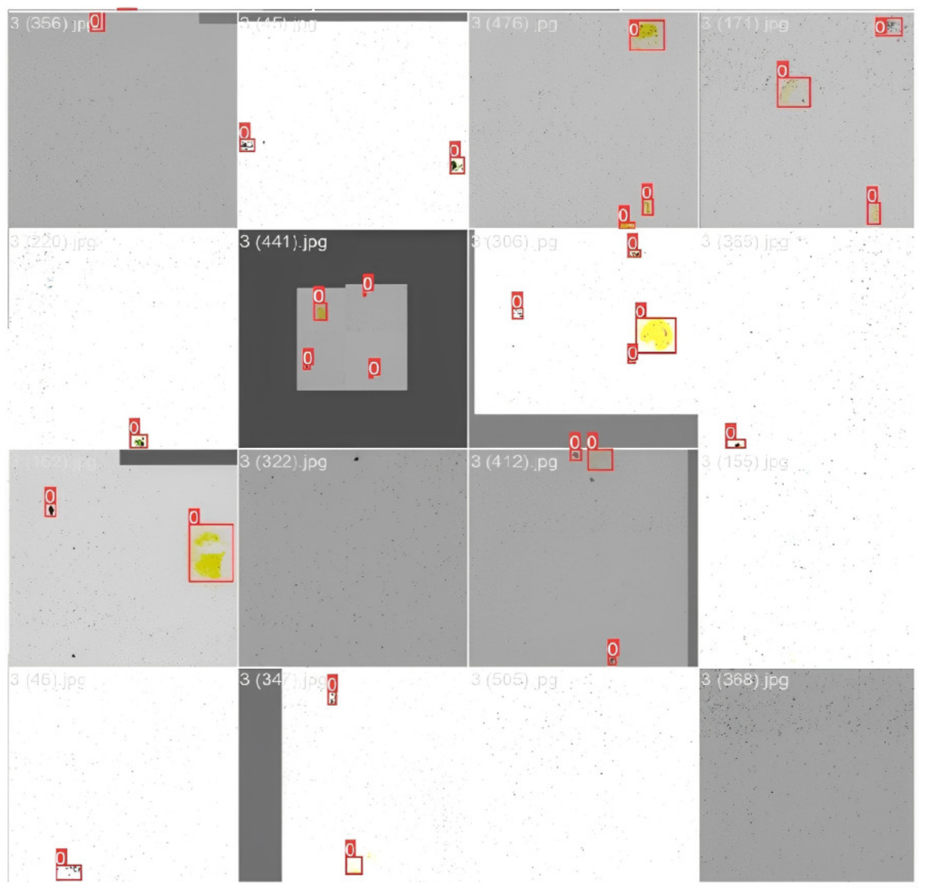
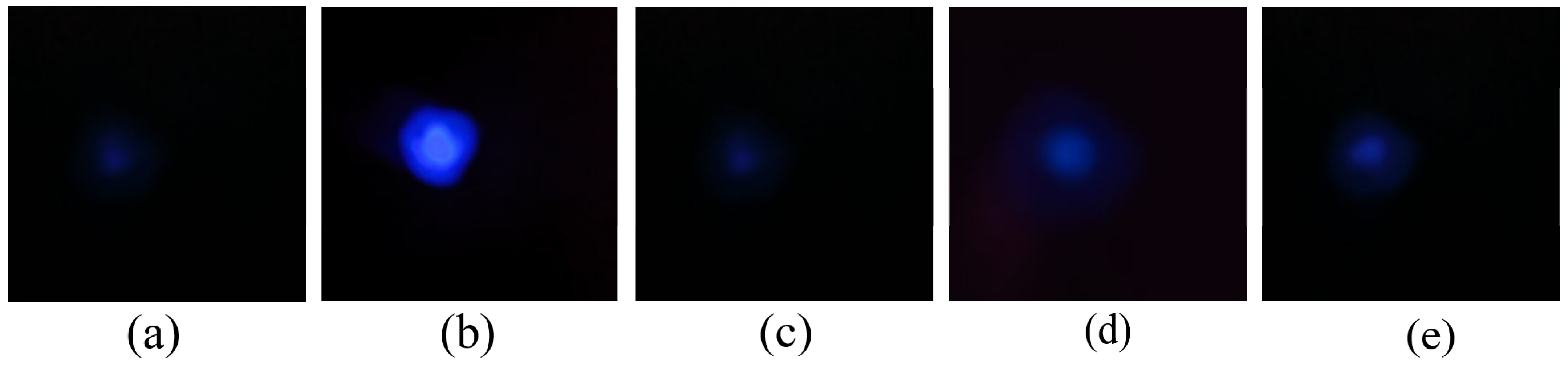
3.1. Materials
3.2. Methods
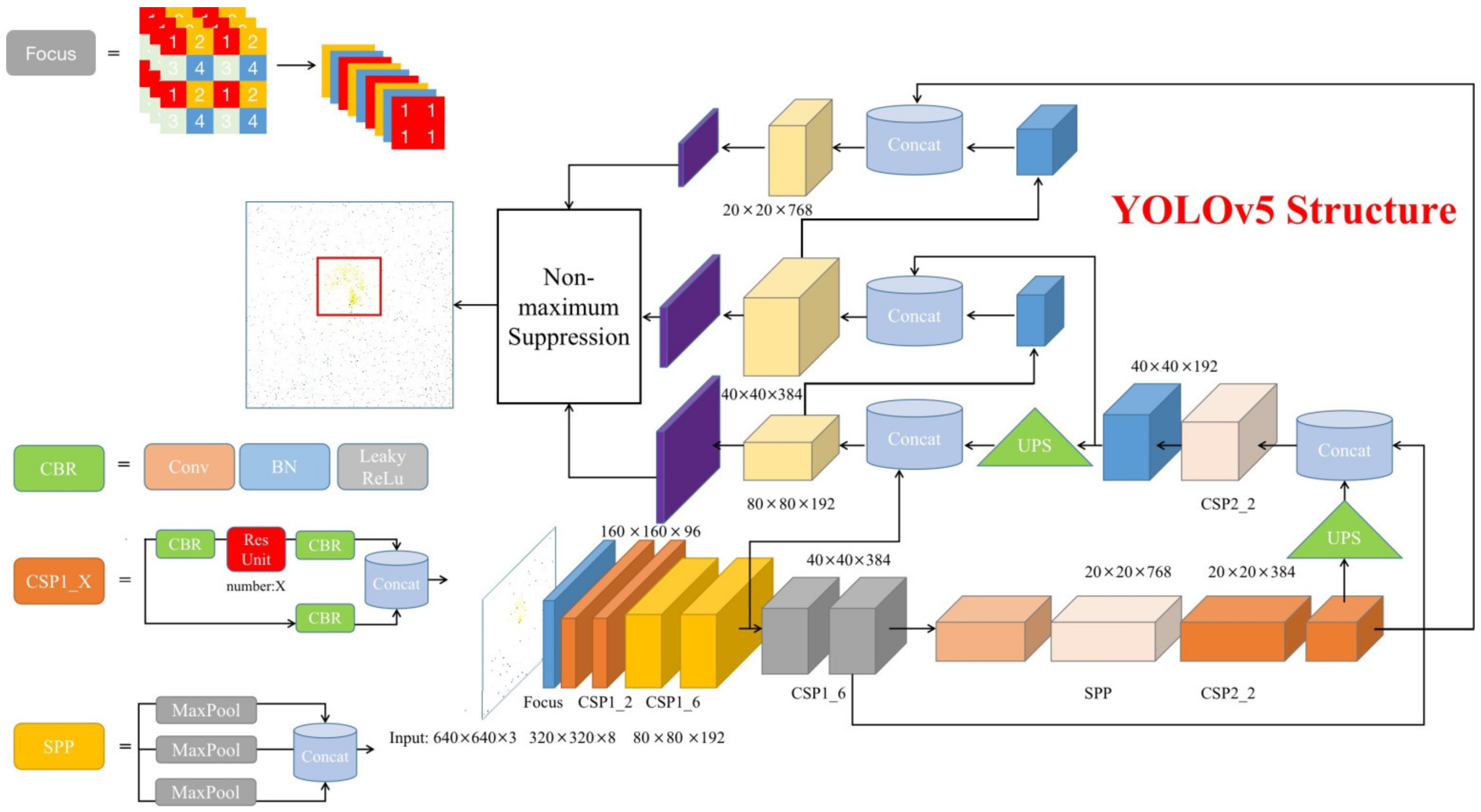
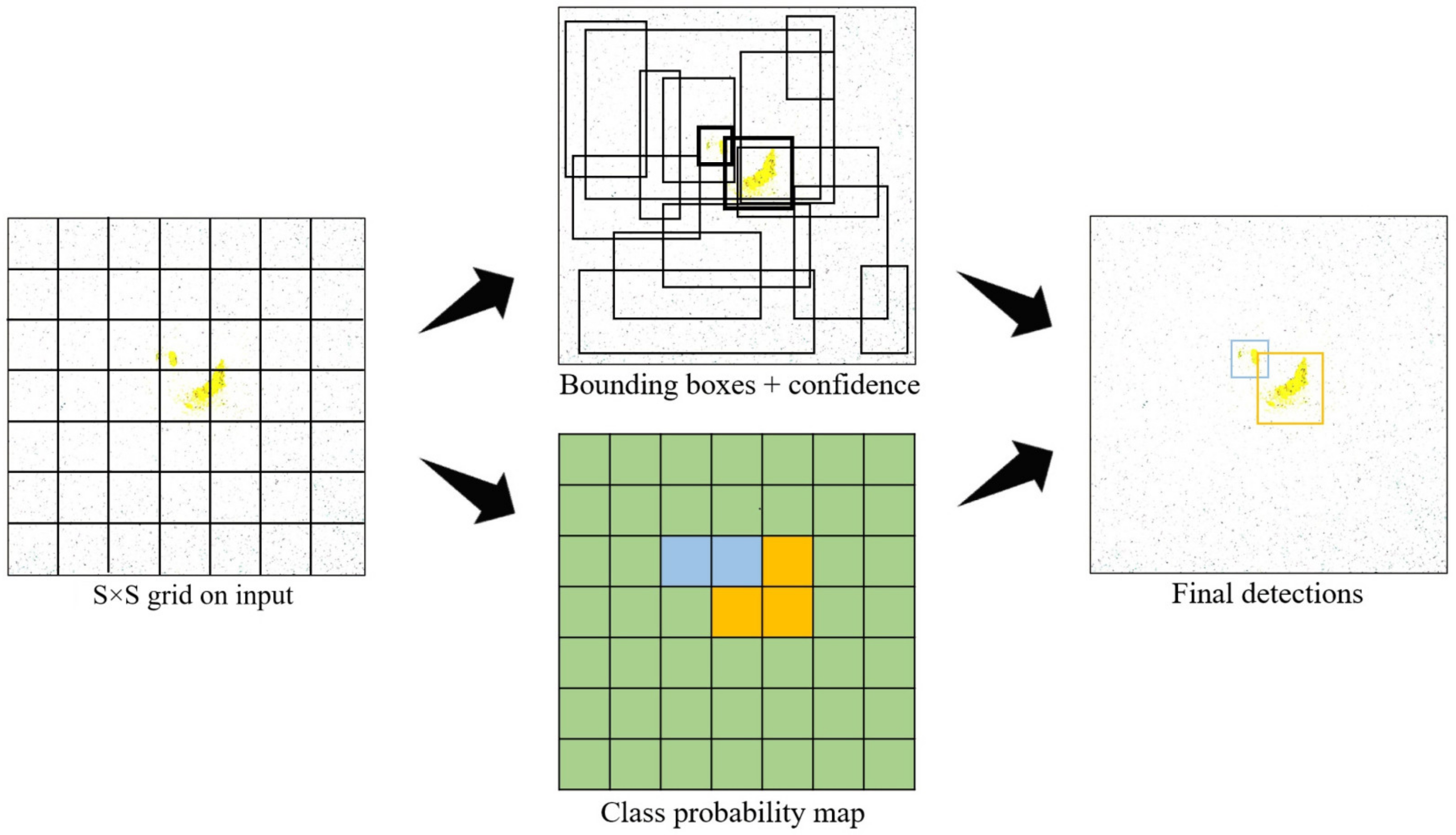
3.2.1. YOLOv5
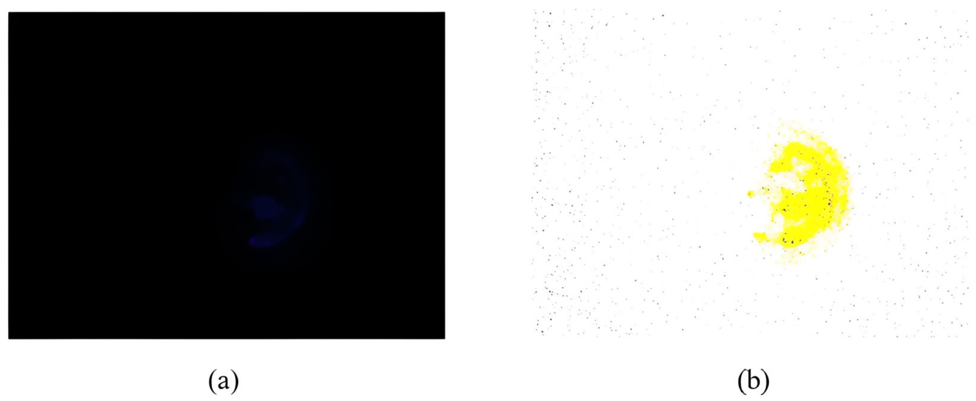
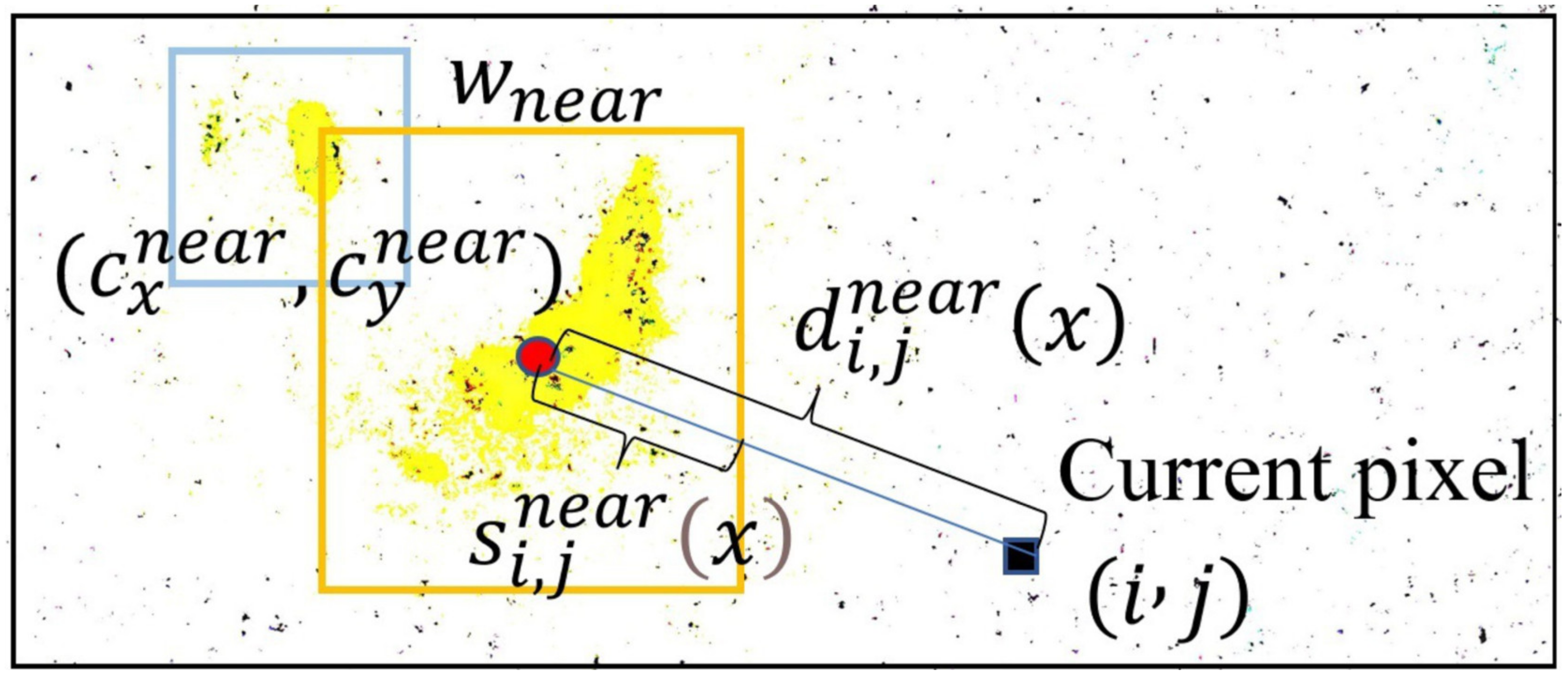
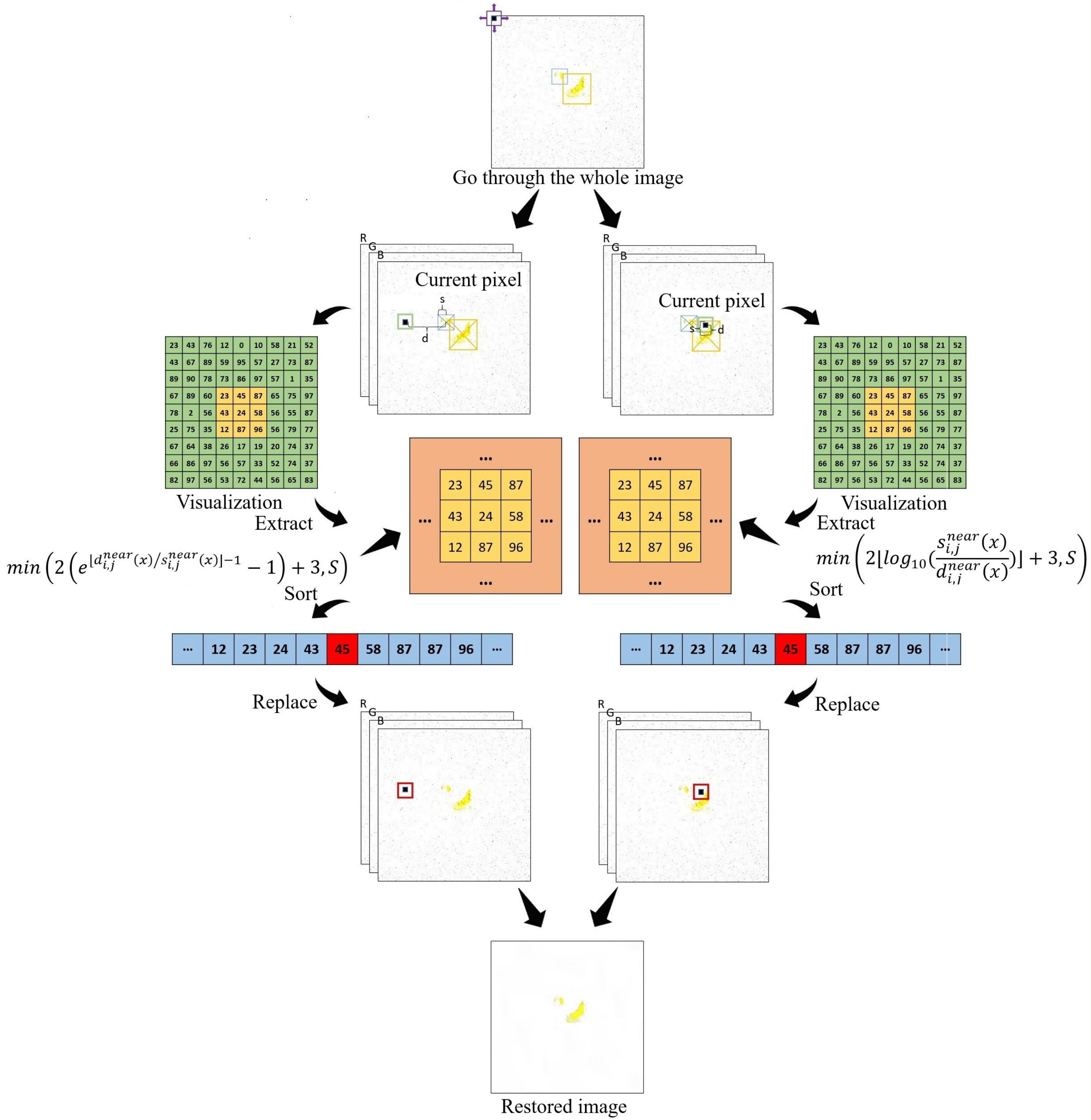
3.2.2. CAMF
| Algorithm 1. Center-Adaptive Median Filter (CAMF). |
For each pixel of the image , do
|
4. Results and Discussion
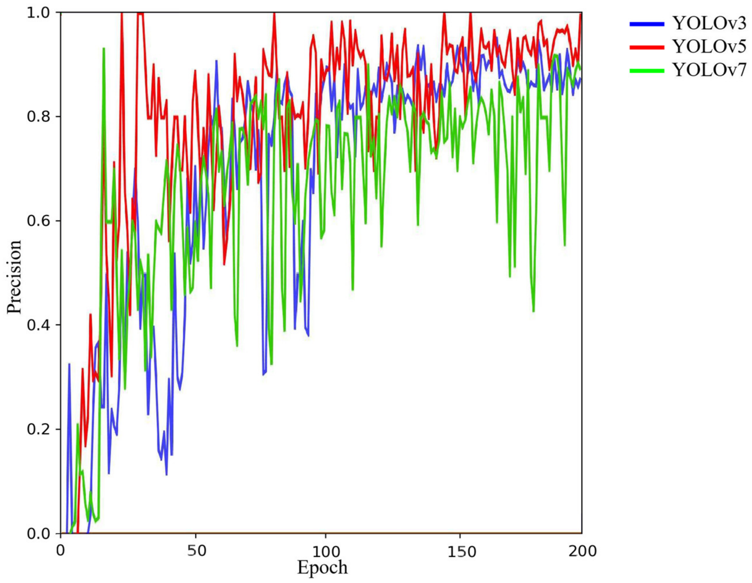
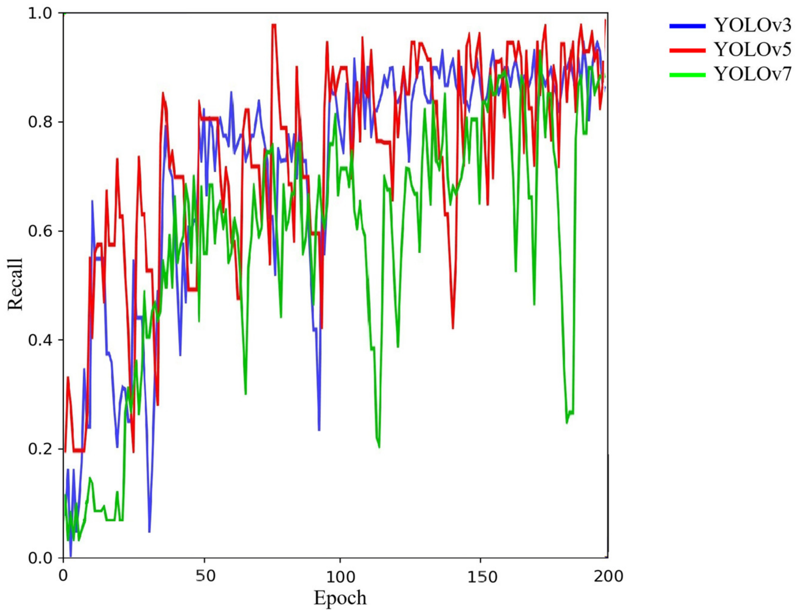
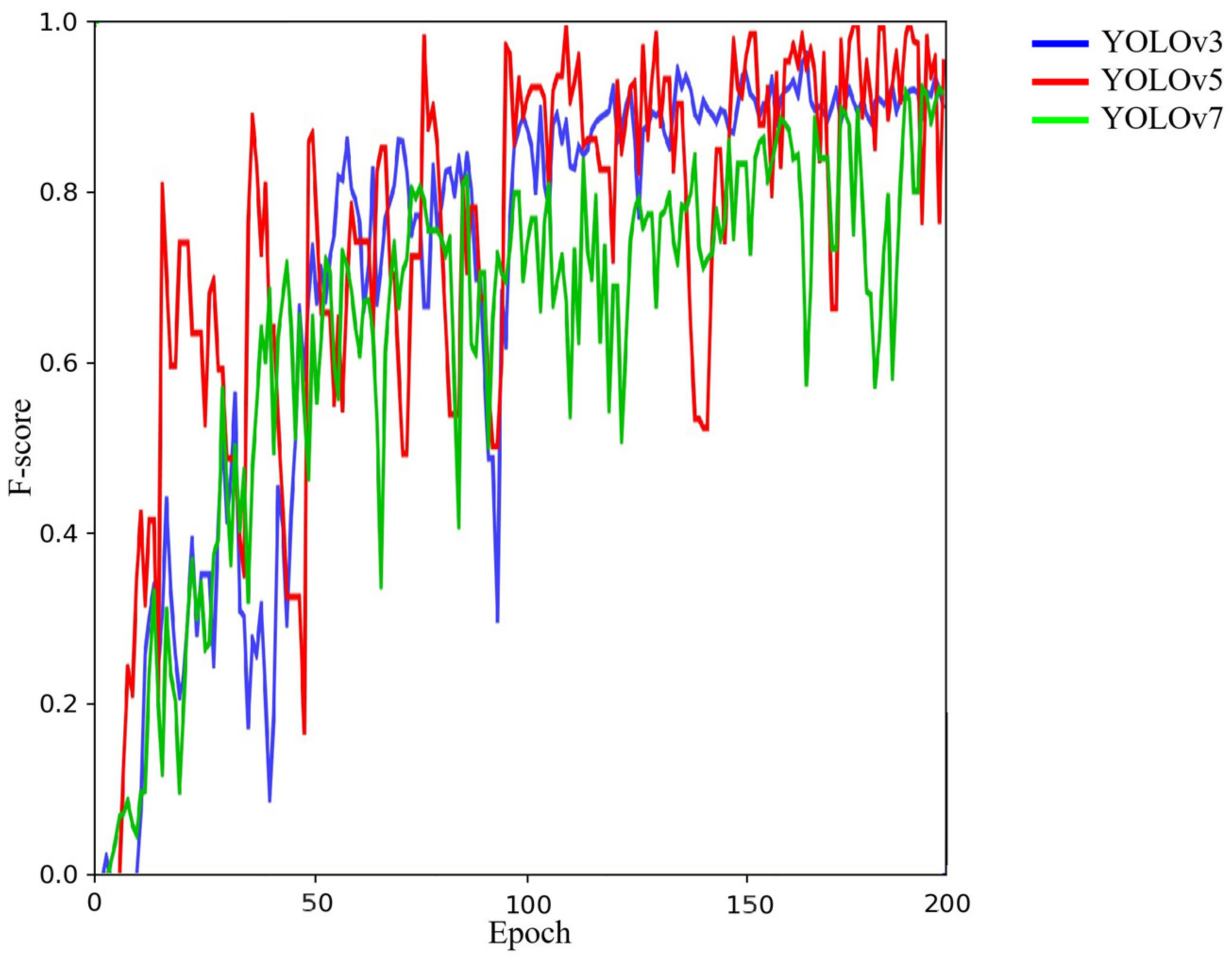
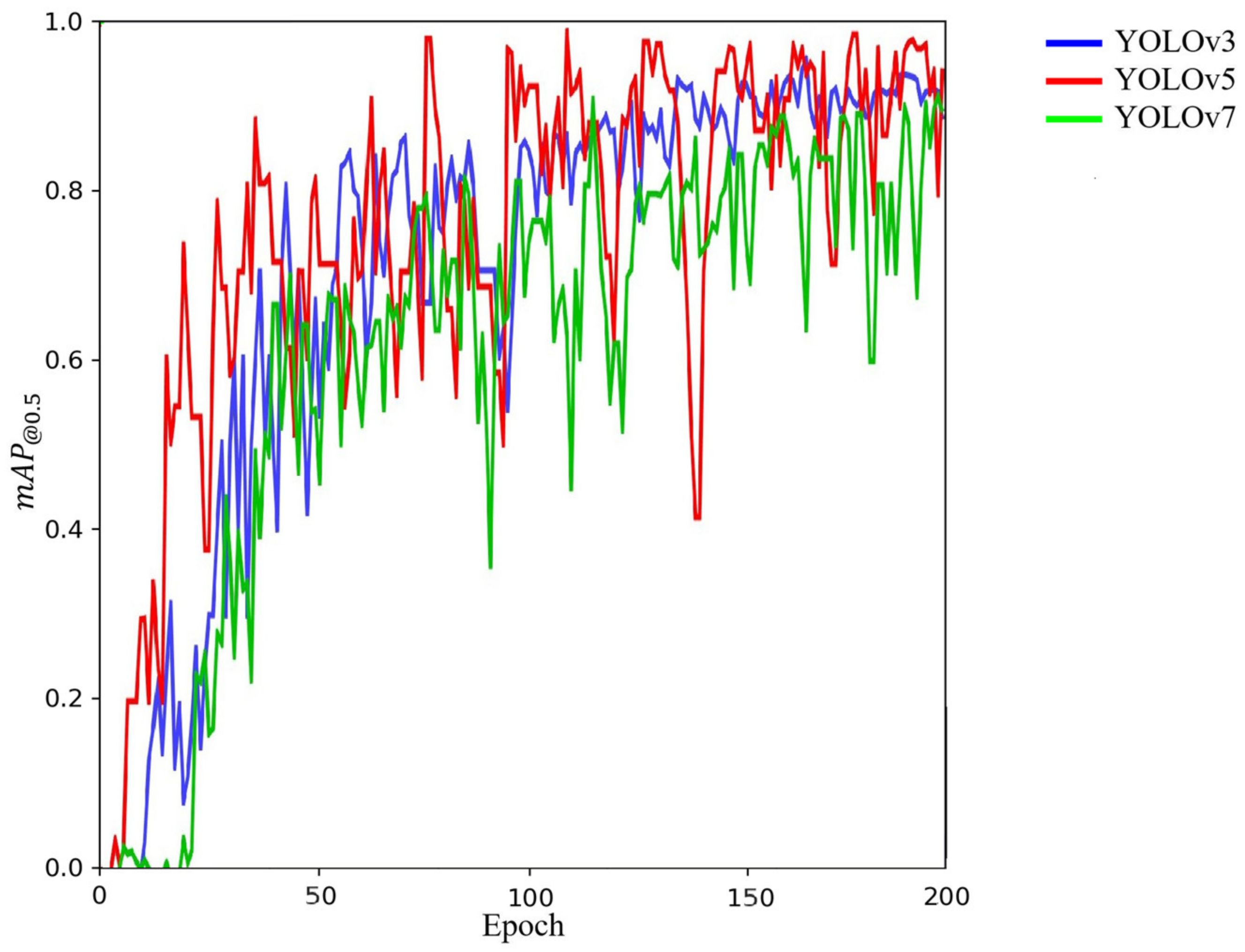
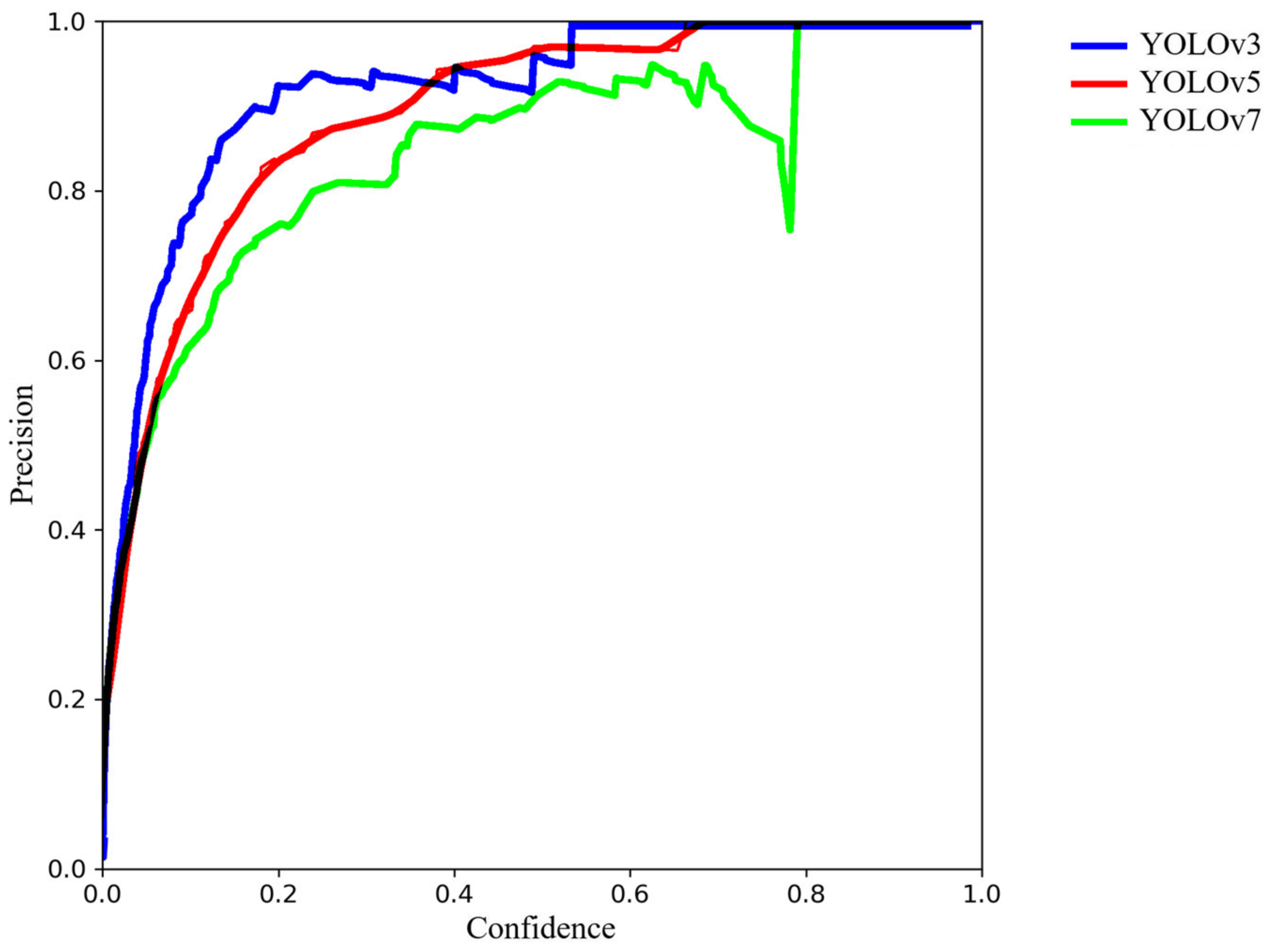
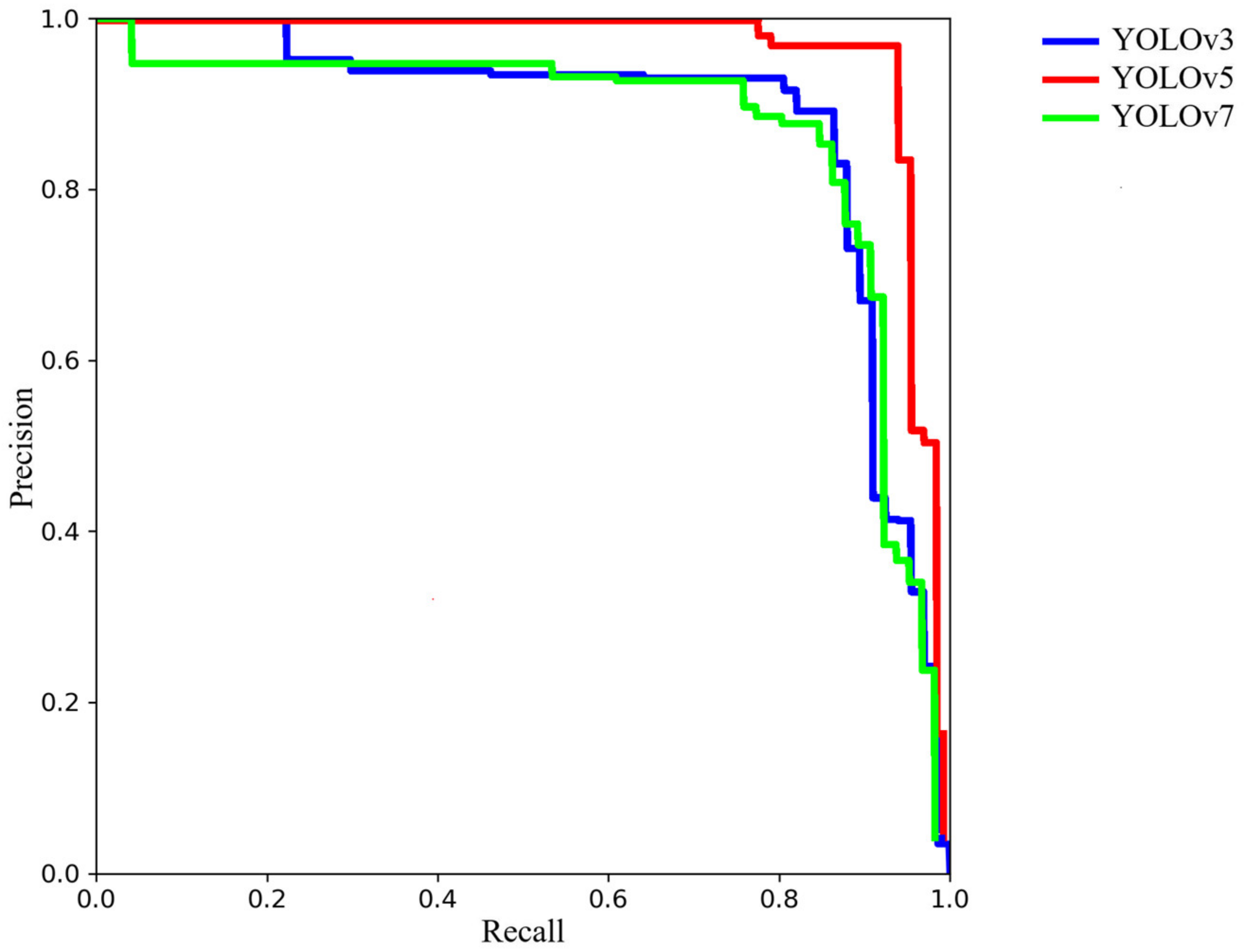
4.1. Comparison between YOLOv3, YOLOv5 and YOLOv7
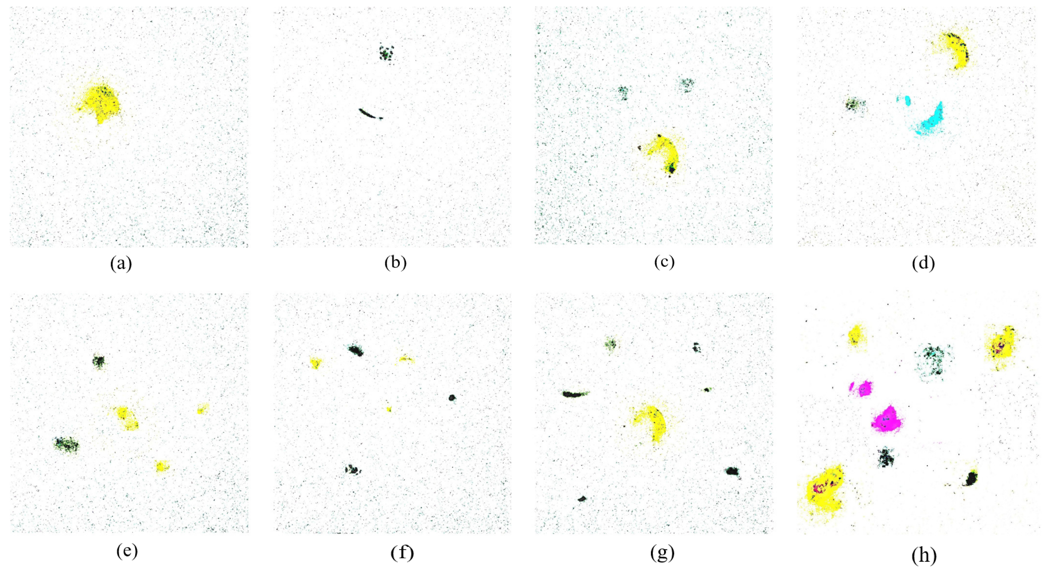
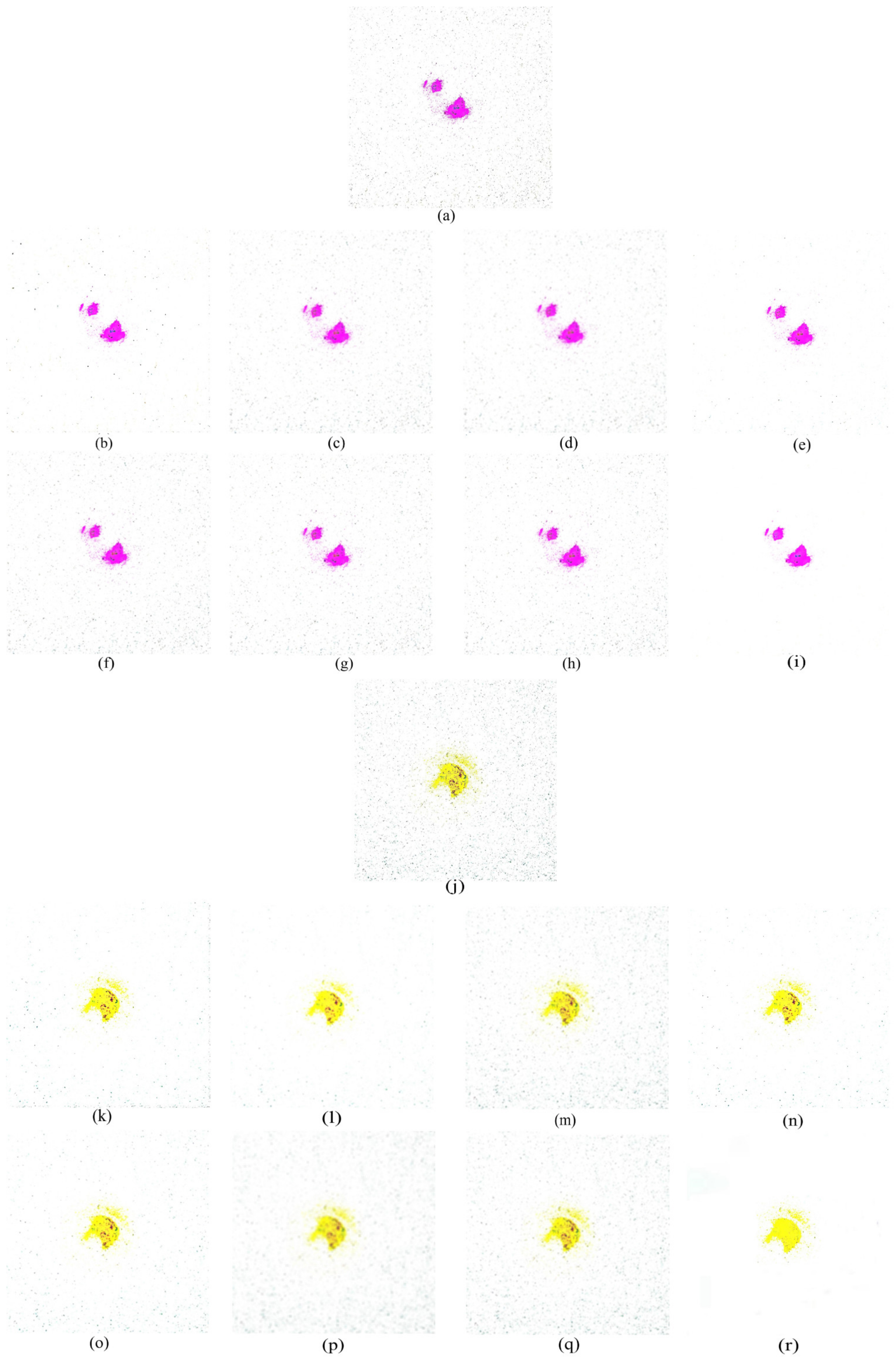
4.2. Comparison between CAMF and Other Filtering Algorithms
5. Conclusions
Author Contributions
Funding
Data Availability Statement
Acknowledgments
Conflicts of Interest
Acronyms
| AIFF | Adaptive Iterative Fuzzy Filter |
| AMF | Adaptive Median Filter |
| AP | Average Precision |
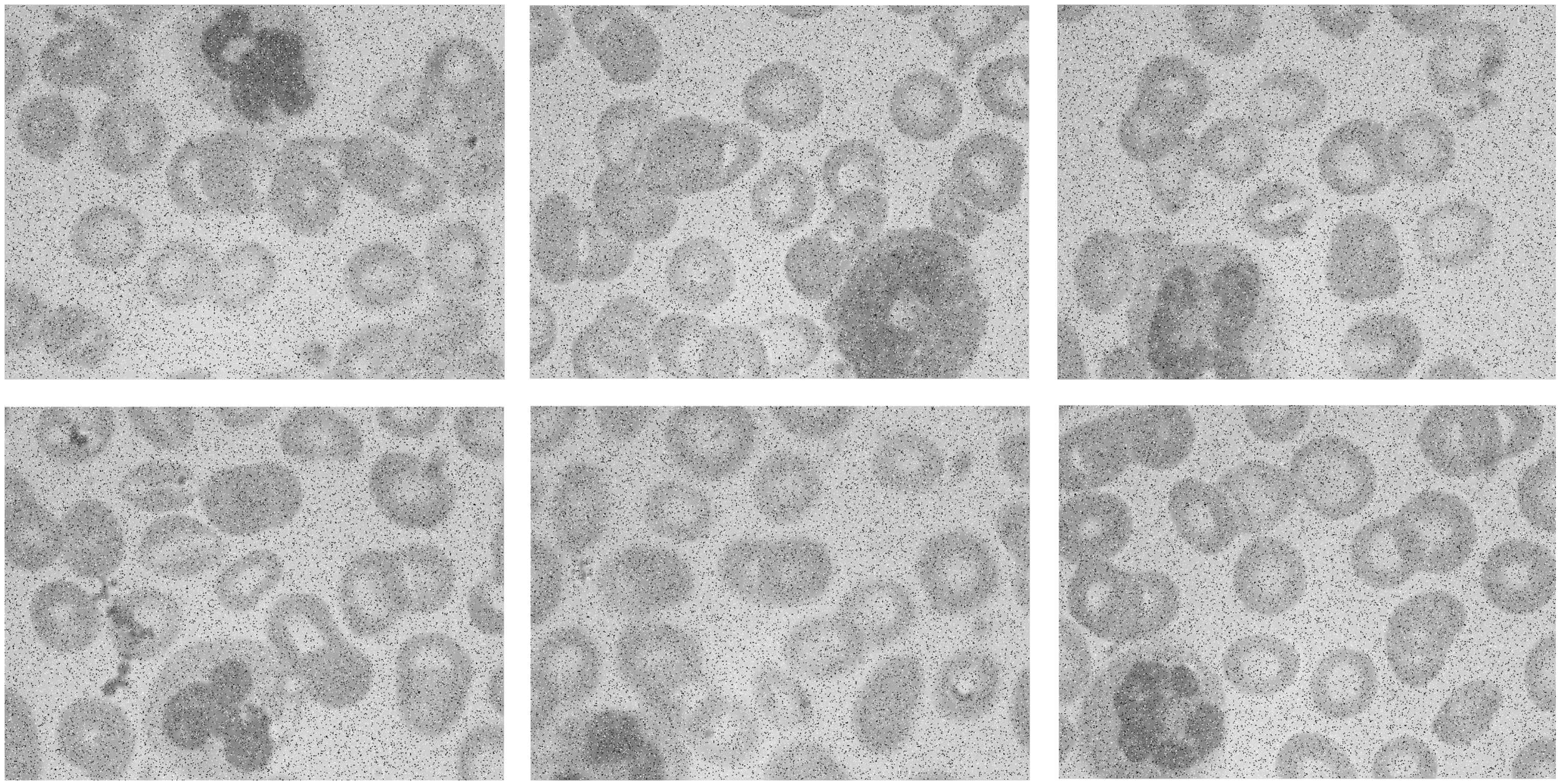
| BC | Blood Cell |
| CAMF | Center-Adaptive Median Filter |
| CSP | Cross Stage Partia |
| CSPNet | Cross Stage Partial Network |
| DAMF | Different Applied Median Filter |
| ECL | Electrochemiluminescence |
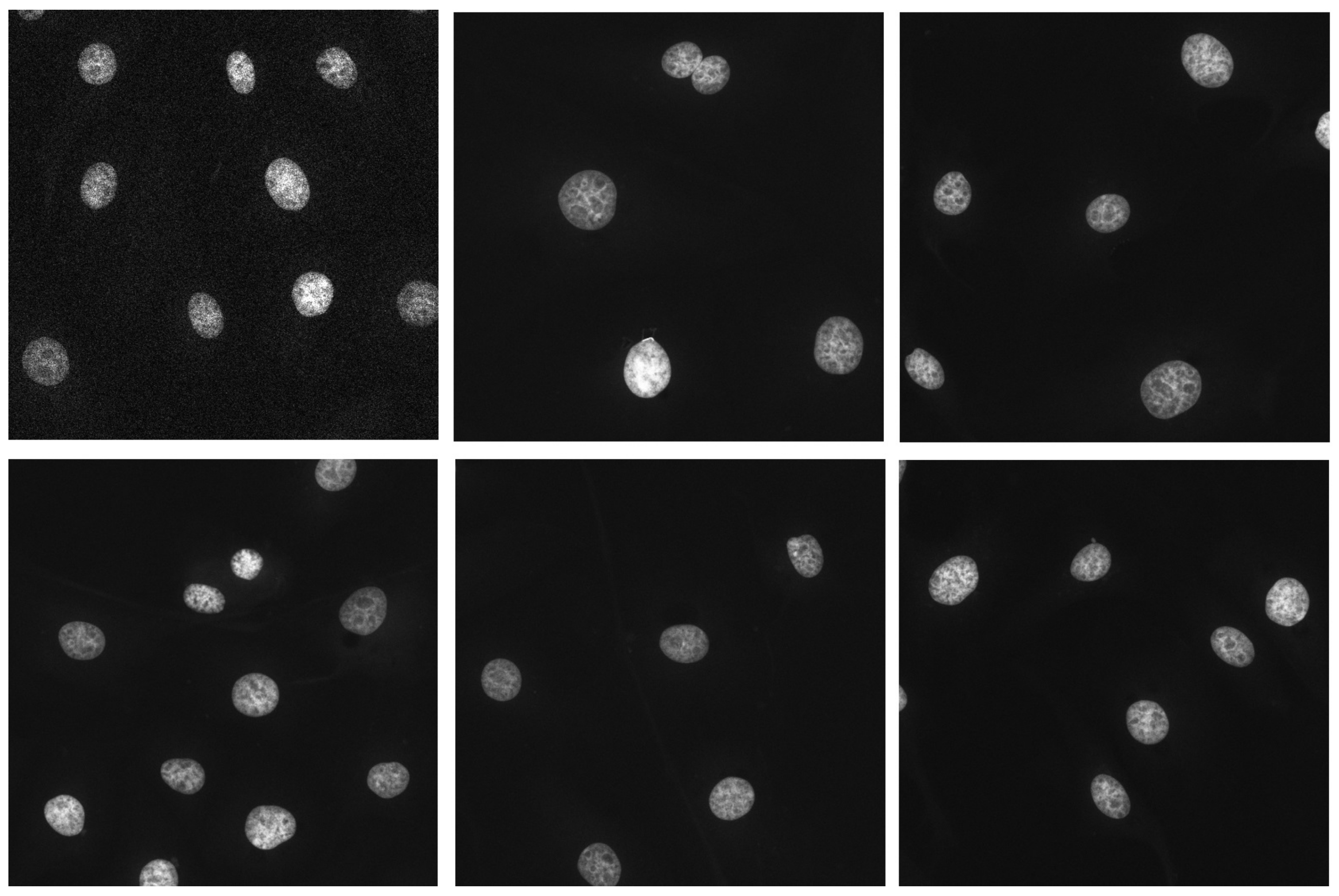
| FMD | Fluorescence Microscopy Denoising |
| FPN | Feature Pyramid Network |
| IEF | Image Enhancement Factor |
| MDBUTMF | Modified Decision-Based Unsymmetric Trimmed Median Filter |
| MF | Median Filter |
| NAFSMF | Noise Adaptive Fuzzy Switching Median Filter |
| PAN | Path Aggregation Network |
| PDBF | Probabilistic Decision Based Filter |
| PSNR | Peak Signal-to-Noise Ratio |
| RepVGG | Reproducible Visual Geometry Group |
| SPN | Salt-and-Pepper Noise |
| SSIM | Structural Similarity |
| YOLO | You Only Look Once |
| YOLOv1 | You Only Look Once version 1 |
| YOLOv3 | You Only Look Once version 3 |
| YOLOv5 | You Only Look Once version 5 |
| YOLOv5s | You Only Look Once version 5 small |
| YOLOv7 | You Only Look Once version 7 |
| mAP | mean Average Precision |
References
- Liu, S.; Yuan, H.; Bai, H.; Zhang, P.; Lv, F.; Liu, L.; Dai, Z.; Bao, J.; Wang, S. Electrochemiluminescence for Electric-Driven Antibacterial Therapeutics. J. Am. Chem. Soc. 2018, 140, 2284–2291. [Google Scholar] [CrossRef] [PubMed]
- Wang, Y.; Zhao, G.; Chi, H.; Yang, S.; Niu, Q.; Wu, D.; Cao, W.; Li, T.; Ma, H.; Wei, Q. Self-Luminescent Lanthanide Metal-Organic Frameworks as Signal Probes in Electrochemiluminescence Immunoassay. J. Am. Chem. Soc. 2021, 13, 504–512. [Google Scholar]
- Huang, W.; Hu, G.; Yao, L.; Yang, Y.; Liang, W.; Yuan, R.; Xiao, D. Matrix Coordination-Induced Electrochemiluminescence Enhancement of Tetraphenylethylene-Based Hafnium Metal–Organic Framework: An Electrochemiluminescence Chromophore for Ultrasensitive Electrochemiluminescence Sensor Construction. Anal. Chem. 2020, 18, 3380–3387. [Google Scholar] [CrossRef] [PubMed]
- Huo, X.-L.; Chen, Y.; Bao, N.; Shi, C.-G. Electrochemiluminescence integrated with paper chromatography for separation and detection of environmental hormones. Sens. Actuator B-Chem. 2021, 334, 129662. [Google Scholar] [CrossRef]
- Jafri, L.; Khan, A.; Siddiqui, A.; Mushtaq, S.; Iqbal, R.; Ghani, F.; Siddiqui, I. Comparison of high performance liquid chromatography, radio immunoassay and electrochemiluminescence immunoassay for quantification of serum 25 hydroxy vitamin D. Clin. Biochem. 2011, 44, 864–868. [Google Scholar] [CrossRef]
- Liu, Z.; Wang, L.; Liu, P.; Zhao, K.; Ye, S.; Liang, G. Rapid, ultrasensitive and non-enzyme electrochemiluminescence detection of hydrogen peroxide in food based on the ssDNA/g-C3N4 nanosheets hybrid. Food Chem. 2021, 357, 129753. [Google Scholar] [CrossRef] [PubMed]
- Peng, L.; Li, P.; Chen, J.; Deng, A.; Li, J. Recent progress in assembly strategies of nanomaterials-based ultrasensitive electrochemiluminescence biosensors for food safety and disease diagnosis. Talanta 2023, 253, 123906. [Google Scholar] [CrossRef]
- Hao, N.; Wang, K. Recent development of electrochemiluminescence sensors for food analysis. Anal. Bioanal. Chem. 2016, 408, 7035–7048. [Google Scholar] [CrossRef]
- Liu, Q.; Fei, A.; Wang, K. An immobilization-free and homogeneous electrochemiluminescence assay for detection of environmental pollutant graphene oxide in water. J. Electroanal. Chem. 2021, 897, 115583. [Google Scholar] [CrossRef]
- Han, Z.; Yang, Z.; Sun, H.; Xu, Y.; Ma, X.; Shan, D.; Chen, J.; Huo, S.; Zhang, Z.; Du, P.; et al. Electrochemiluminescence Platforms Based on Small Water-Insoluble Organic Molecules for Ultrasensitive Aqueous-Phase Detection. Angew. Chem. Int. Ed. Engl. 2019, 58, 5915–5919. [Google Scholar] [CrossRef]
- Busa, L.; Mohammadi, S.; Maeki, M.; Ishida, A.; Tani, H.; Tokeshi, M. Advances in Microfluidic Paper-Based Analytical Devices for Food and Water Analysis. Micromachines 2016, 7, 86. [Google Scholar] [CrossRef] [PubMed]
- Zhang, J.; Arbault, S.; Sojic, N.; Jiang, D. Electrochemiluminescence Imaging for Bioanalysis. Rev. Anal. Chem. 2019, 12, 275–295. [Google Scholar] [CrossRef] [PubMed]
- Díez-Buitrago, B.; Saa, L.; Briz, N.; Pavlov, V. Development of portable CdS QDs screen-printed carbon electrode platform for electrochemiluminescence measurements and bioanalytical applications. Talanta 2021, 225, 122029. [Google Scholar] [CrossRef]
- Zanut, A.; Fiorani, A.; Canola, S.; Saito, T.; Ziebart, N.; Rapino, S.; Rebeccani, S.; Barbon, A.; Irie, T.; Josel, H.P.; et al. Insights into the mechanism of coreactant electrochemiluminescence facilitating enhanced bioanalytical performance. Nat. Commun. 2020, 11, 2668. [Google Scholar] [CrossRef] [PubMed]
- Brown, K.; Allan, P.; Francis, P.S.; Dennany, L. Psychoactive Substances and How to Find Them: Electrochemiluminescence as a Strategy for Identification and Differentiation of Drug Species. J. Electrochem. Soc. 2020, 167, 166502. [Google Scholar] [CrossRef]
- Zhang, Z.; Du, P.; Pu, G.; Wei, L.; Wu, Y.; Guo, J.; Lu, X. Utilization and prospects of electrochemiluminescence for characterization, sensing, imaging and devices. Mater. Chem. Front. 2019, 3, 2246–2257. [Google Scholar] [CrossRef]
- Chu, H.; Guo, W.; Di, J.; Wu, Y.; Tu, Y. Study on Sensitization from Reactive Oxygen Species for Electrochemiluminescence of Luminol in Neutral Medium. Electroanalysis 2009, 21, 1630–1635. [Google Scholar] [CrossRef]
- Zong, L.-P.; Ruan, L.-Y.; Li, J.; Marks, R.S.; Wang, J.-S.; Cosnier, S.; Zhang, X.-J.; Shan, D. Fe-MOGs-based enzyme mimetic and its mediated electrochemiluminescence for in situ detection of H2O2 released from Hela cells. Biosens. Bioelectron. 2021, 184, 113216. [Google Scholar] [CrossRef]
- Liu, T.; He, J.; Lu, Z.; Sun, M.; Wu, M.; Wang, X.; Jiang, Y.; Zou, P.; Rao, H.; Wang, Y. A visual electrochemiluminescence molecularly imprinted sensor with Ag+@UiO-66-NH2 decorated CsPbBr3 perovskite based on smartphone for point-of-care detection of nitrofurazone. Chem. Eng. J. 2022, 429, 132462. [Google Scholar] [CrossRef]
- Zhang, Y.; Cui, Y.; Sun, M.; Wang, T.; Liu, T.; Dai, X.; Zou, P.; Zhao, Y.; Wang, X.; Wang, Y.; et al. Deep learning-assisted smartphone-based molecularly imprinted electrochemiluminescence detection sensing platform: Protable device and visual monitoring furosemide. Biosens. Bioelectron. 2022, 209, 114262. [Google Scholar] [CrossRef]
- Goyal, P.; Khanna, N.; Dosad, J.; Gupta, M. Impact of neighborhood size on median filter based color filter array interpolation. Math. Eng. Sci. Aerosp. 2014, 5, 265–274. [Google Scholar]
- Dong, H.; Zhao, L.; Shu, Y.; Neal, N. X-ray image denoising based on wavelet transform and median filter. Appl. Math. Nonlinear Sci. 2020, 5, 435–442. [Google Scholar] [CrossRef]
- Ma, C.; Lv, X.; Ao, J. Difference based median filter for removal of random value impulse noise in images. PLoS ONE 2022, 17, e0264793. [Google Scholar] [CrossRef]
- Wang, S.; Liu, Q.; Xia, Y.; Dong, P.; Luo, J.; Huang, Q.; Feng, D.D. Dictionary learning based impulse noise removal via L1–L1 minimization. Signal Process. 2013, 93, 2696–2708. [Google Scholar] [CrossRef]
- Panetta, K.; Bao, L.; Agaian, S. A New Unified Impulse Noise Removal Algorithm Using a New Reference Sequence-to-Sequence Similarity Detector. IEEE Access 2018, 6, 37225–37236. [Google Scholar] [CrossRef]
- Hwang, H.; Haddad, R.A. Adaptive median filters: New algorithms and results. IEEE Trans. Image Process. 1995, 4, 499–502. [Google Scholar] [CrossRef] [Green Version]
- Wang, X.; Hou, R.; Gao, X.; Xin, B. Research on Yarn Diameter and Unevenness Based on an Adaptive Median Filter Denoising Algorithm. Fibres Text. East. Eur. 2020, 28, 36–41. [Google Scholar] [CrossRef]
- Tripathy, S.; Swarnkar, T. Performance observation of mammograms using an improved dynamic window based adaptive median filter. J. Discret. Math. Sci. Cryptogr. 2020, 23, 167–175. [Google Scholar] [CrossRef]
- Ahmed, F.; Das, S. Removal of High-Density Salt-and-Pepper Noise in Images With an Iterative Adaptive Fuzzy Filter Using Alpha-Trimmed Mean. IEEE Trans. Fuzzy Syst. 2014, 22, 1352–1358. [Google Scholar] [CrossRef]
- Sheela, C.; Suganthi, G. An efficient denoising of impulse noise from MRI using adaptive switching modified decision based unsymmetric trimmed median filter. Biomed. Signal Process. Control. 2020, 55, 101657. [Google Scholar] [CrossRef]
- Toh, K.K.V.; Isa, N.A.M. Noise Adaptive Fuzzy Switching Median Filter for Salt-and-Pepper Noise Reduction. IEEE Signal Process. Lett. 2010, 17, 281–284. [Google Scholar] [CrossRef] [Green Version]
- Wang, Y.; Wang, J.; Song, X.; Han, L. An Efficient Adaptive Fuzzy Switching Weighted Mean Filter for Salt-and-Pepper Noise Removal. IEEE Signal Process. Lett. 2016, 23, 1582–1586. [Google Scholar] [CrossRef]
- Lee, J.Y.; Jung, S.; Kim, P. Adaptive switching filter for impulse noise removal in digital content. Soft Comput. 2018, 22, 1445–1455. [Google Scholar] [CrossRef]
- Erkan, U.; Gökrem, L.; Enginoğlu, S. Different applied median filter in salt and pepper noise. Comput. Electr. Eng. 2018, 70, 789–798. [Google Scholar] [CrossRef]
- Deivalakshmi, S.; Palanisamy, P. Removal of high density salt and pepper noise through improved tolerance based selective arithmetic mean filtering with wavelet thresholding. AEU-Int. J. Electron. Commun. 2016, 70, 757–776. [Google Scholar] [CrossRef]
- Balasubramanian, G.; Chilambuchelvan, A.; Vijayan, S.; Gowrison, G. Probabilistic decision based filter to remove impulse noise using patch else trimmed median. AEU-Int. J. Electron. Commun. 2016, 70, 471–481. [Google Scholar] [CrossRef]
- Sen, A.; Rout, N. Probabilistic Decision Based Improved Trimmed Median Filter to Remove High-Density Salt and Pepper Noise. Pattern Recognit. Image Anal. 2020, 30, 401–415. [Google Scholar] [CrossRef]
- Redmon, J.; Divvala, S.; Girshick, R.; Farhadi, A. You Only Look Once: Unified, Real-Time Object Detection. In Proceedings of the IEEE Conference on Computer Vision and Pattern Recognition, Las Vegas, NV, USA, 27–30 June 2016; pp. 779–788. [Google Scholar]
- Mohiyuddin, A.; Basharat, A.; Ghani, U.; Peter, V.; Abbas, S.; Naeem, O.; Rizwan, M. Breast Tumor Detection and Classification in Mammogram Images Using Modified YOLOv5 Network. Comput. Math. Methods Med. 2022, 2022, 1359019. [Google Scholar] [CrossRef] [PubMed]
- Redmon, J.; Farhadi, A. Yolov3: An incremental improvement. arXiv 2018, arXiv:1804.02767. [Google Scholar]
- Ding, X.; Zhang, X.; Ma, N.; Han, J.; Ding, G.; Sun, J. RepVGG: Making VGG-Style ConvNets Great Again. In Proceedings of the IEEE/CVF Conference on Computer Vision and Pattern Recognition (CVPR), Virtual, 19–25 June 2021; IEEE Trans: Nashville, TN, USA, 2021. [Google Scholar]
- Wang, C.Y.; Bochkovskiy, A.; Liao, H. YOLOv7: Trainable bag-of-freebies sets new state-of-the-art for real-time object detectors. arXiv 2022, arXiv:2207.02696. [Google Scholar]
- Khasawneh, N.; Fraiwan, M.; Fraiwan, L. Detection of K-complexes in EEG signals using deep transfer learning and YOLOv3. Cluster Comput. 2022. [Google Scholar] [CrossRef]
- Ali, L.; Alnajjar, F.; Parambil, M.; Younes, M.; Abdelhalim, Z.; Aljassmi, H. Development of YOLOv5-Based Real-Time Smart Monitoring System for Increasing Lab Safety Awareness in Educational Institutions. Sensors 2022, 22, 8820. [Google Scholar] [CrossRef] [PubMed]
- Sozzi, M.; Cantalamessa, S.; Cogato, A.; Kayad, A.; Marinello, F. Automatic Bunch Detection in White Grape Varieties Using YOLOv3, YOLOv4, and YOLOv5 Deep Learning Algorithms. Agronomy 2022, 12, 319. [Google Scholar] [CrossRef]
- Yang, Y. Drone-View Object Detection Based on the Improved YOLOv5. In Proceedings of the 2022 IEEE International Conference on Electrical Engineering, Big Data and Algorithms (EEBDA), Changchun, China, 25–27 February 2022; pp. 612–617. [Google Scholar]
- Cao, M.; Fu, H.; Zhu, J.; Cai, C. Lightweight tea bud recognition network integrating GhostNet and YOLOv5. Math. Biosci. Eng. 2022, 19, 12897–12914. [Google Scholar] [CrossRef] [PubMed]
- Chen, K.; Li, H.; Li, C.; Zhao, X.; Wu, S.; Duan, Y.; Wang, J. An Automatic Defect Detection System for Petrochemical Pipeline Based on Cycle-GAN and YOLO v5. Sensors 2022, 22, 7907. [Google Scholar] [CrossRef] [PubMed]
- Wang, C.Y.; Liao HY, M.; Wu, Y.H.; Chen, P.Y.; Hsieh, J.W.; Yeh, I.H. CSPNet: A new backbone that can enhance learning capability of CNN. In Proceedings of the IEEE/CVF Conference on Computer Vision and Pattern Recognition Workshops, Seattle, WA, USA, 14–19 June 2020; pp. 390–391. [Google Scholar]
- Wang, Z.; Bovik, A.C.; Sheikh, H.R.; Simoncelli, E.P. Image quality assessment: From error visibility to structural similarity. IEEE Trans. Image Process. 2004, 13, 600–612. [Google Scholar] [CrossRef] [PubMed] [Green Version]
- Djurović, I. Combination of the adaptive Kuwahara and BM3D filters for filtering mixed Gaussian and impulsive noise. Signal Image Video Process. 2017, 11, 753–760. [Google Scholar] [CrossRef]


| Filter Algorithms | PSNR (dB) | IEF | SSIM |
|---|---|---|---|
| IMF | 30.59 | 341.74 | 0.935 |
| MF | 37.90 | 425.83 | 0.931 |
| MDBUTMF | 32.34 | 519.72 | 0.929 |
| NAFSMF | 31.98 | 434.61 | 0.922 |
| DAMF | 36.01 | 490.71 | 0.920 |
| AIFF | 34.23 | 407.77 | 0.919 |
| PDBF | 35.07 | 231.09 | 0.912 |
| CAMF (Ours) | 40.47 | 613.28 | 0.939 |
| Filter Algorithms | Time (s) |
|---|---|
| IMF | 4.28 |
| MF | 3.70 |
| MDBUTMF | 5.69 |
| NAFSMF | 6.09 |
| DAMF | 1.23 |
| AIFF | 6.47 |
| PDBF | 4.50 |
| CAMF (Ours) | 4.02 |
| Dataset | Filter Algorithms | PSNR (dB) | IEF | SSIM |
|---|---|---|---|---|
| FMD | CAMF | 40.61 | 589.73 | 0.932 |
| Blood Cell | CAMF | 39.68 | 609.73 | 0.933 |
Disclaimer/Publisher’s Note: The statements, opinions and data contained in all publications are solely those of the individual author(s) and contributor(s) and not of MDPI and/or the editor(s). MDPI and/or the editor(s) disclaim responsibility for any injury to people or property resulting from any ideas, methods, instructions or products referred to in the content. |
© 2023 by the authors. Licensee MDPI, Basel, Switzerland. This article is an open access article distributed under the terms and conditions of the Creative Commons Attribution (CC BY) license (https://creativecommons.org/licenses/by/4.0/).
Share and Cite
Yang, J.; Chen, J.; Li, J.; Dai, S.; He, Y. An Improved Median Filter Based on YOLOv5 Applied to Electrochemiluminescence Image Denoising. Electronics 2023, 12, 1544. https://doi.org/10.3390/electronics12071544
Yang J, Chen J, Li J, Dai S, He Y. An Improved Median Filter Based on YOLOv5 Applied to Electrochemiluminescence Image Denoising. Electronics. 2023; 12(7):1544. https://doi.org/10.3390/electronics12071544
Chicago/Turabian StyleYang, Jun, Junyang Chen, Jun Li, Shijie Dai, and Yihui He. 2023. "An Improved Median Filter Based on YOLOv5 Applied to Electrochemiluminescence Image Denoising" Electronics 12, no. 7: 1544. https://doi.org/10.3390/electronics12071544