Stretching Deep Architectures: A Deep Learning Method without Back-Propagation Optimization

Abstract

In recent years, researchers have proposed many deep learning algorithms for data representation learning. However, most deep networks require extensive training data and a lot of training time to obtain good results. In this paper, we propose a novel deep learning method based on stretching deep architectures that are composed of stacked feature learning models. Hence, the method is called “stretching deep architectures” (SDA). In the feedforward propagation of SDA, feature learning models are firstly stacked and learned layer by layer, and then the stretching technique is applied to map the last layer of the features to a high-dimensional space. Since the feature learning models are optimized effectively, and the stretching technique can be easily calculated, the training of SDA is very fast. More importantly, the learning of SDA does not need back-propagation optimization, which is quite different from most of the existing deep learning models. We have tested SDA in visual texture perception, handwritten text recognition, and natural image classification applications. Extensive experiments demonstrate the advantages of SDA over traditional feature learning models and related deep learning models.

1. Introduction

Data representation plays an essential role in many learning tasks, such as image understanding and document analysis [1,2,3]. In the literature, many approaches have been proposed to bridge the gap between low-level inputs and high-level concepts [4]. For instance, latent semantic analysis (LSA) is an approach to extracting semantic information from texts using the singular value decomposition (SVD) [5,6], while probabilistic LSA (PLSA) is its probabilistic version. However, due to low-level representation, most of the previous methods cannot perform well in complex applications. In recent years, deep learning has attracted much attention in the areas related to artificial intelligence. Many papers have shown that deep architectures are more effective than traditional shallow representation learning methods [7,8,9,10,11,12,13,14]. However, in order to obtain good learning results, almost all the existing deep networks need a large number of training samples and a long training period.

In this work, we focus on representation learning for visual texture perception and image understanding. Texture is a basic image attribute and is often used to describe various surface features. A textural region may be described as “regular”, “vertically oriented”, or “rough”. As shown in Figure 1, 20 example images from different categories of procedural textures are presented. According to the appearance of texture, observers can determine whether two objects are made of the same substance, and whether two texture images display the same object. We can locate the intervening border by detecting different textures of two adjacent regions. Texture-defined boundaries are also helpful for image segmentation and shape recognition. Moreover, as a special type of texture, procedural textures are generated by mathematical models and widely used to produce large-scale and realistic scenes, which can bring wonderful visual effects. The advantage of using procedural texture is that texture images with arbitrary sizes can be efficiently generated by simply adjusting the model parameters.

In the areas of image understanding, virtual reality, computer graphics, and so on, visual texture perception is a very popular and important research direction. It seeks to discover a semantic space to bridge the gap between low-level texture images and high-level perceptual concepts. Over the past two decades, lots of papers on visual texture perception have been published to explore the influence of texture itself and the fundamental mechanism of the human visual system [15,16,17,18,19]. Particularly, in [17,19], researchers found that three-dimensional representations are sufficient for both natural and artificial textures. Additionally, several psychophysical tests on statistical characterizations of texture have been conducted [20,21]. Density and kurtosis are found to be the most sensitive to the observers, respectively. However, observers have only estimated the perceptual features with very few texture images (e.g., Rao and Lohse use only 56 texture images to organize their psychological test [17]), and moreover, the importance of semantic structure underlying the perceptual features is underestimated.

In order to overcome the above shortcomings, we have reorganized a series of psychophysical experiments and numerical tests [22]. A total of 81 observers have estimated texture perception features for 450 texture images generated by 23 procedural texture models [23]. Similar to [17], 12 perceptual features are found to be able to describe texture images relevant to the observers’ perceptions. They are randomness, direction, contrast, repetitiveness, granularity, roughness, density, structural complexity, coarseness, uniformity, orientation, and regularity. Hence, each texture image in this work is represented by a 12-dimensional vector, corresponding to 12 perceptual features, respectively. Furthermore, to learn the effective representations of the texture perceptual features, we adopt the idea of deep learning in this paper.

Before deep learning was proposed in 2006 [7], principal components analysis (PCA) [24], linear discriminant analysis (LDA) [25], and many other feature learning models were proposed and widely used to learn effective representations of data. However, most of these models cannot perform well because their architecture is not deep enough [26,27].

Recently, deep neural networks have been commonly used to deal with complex image understanding problems [7,28]. Particularly, in the ImageNet large-scale visual recognition challenge-2012 (ILSVRC2012), Hinton and their students developed the “AlexNet” model and won the object recognition and detection tasks [29]; in the ICDAR Chinese handwriting recognition competition, deep learning models have shown superiority over traditional feature learning methods on both isolated character recognition and handwritten text recognition tasks [30]. Specifically, convolutional neural networks (CNNs) are deeply researched and widely applied to object recognition and detection tasks [31,32,33]. Recently, the attention mechanism and vision transformer (ViT) models have shown state-of-the-art results, even better results than CNNs, on many image classification applications with a relatively large scale of data [34,35]. Despite the excellent performances of deep neural networks, they have common problems: they generally need a large amount of training samples and a long training time.

In order to fully exploit the advantages of both the traditional feature learning models and deep architectures, in this paper, we propose a novel deep learning framework called stretching deep architectures (SDA). In this work, the deep network is not a previous neural architecture. Specifically, the SDA architecture is composed of shallow feature learning modules. For concreteness, we select seven feature learning models to use, which are PCA, probabilistic principal components analysis (PPCA) [36], Sammon mapping (Sammon) [37], stochastic neighbor embedding (SNE) [38], multidimensional scaling (MDS) [39], LDA [25], and marginal Fisher analysis (MFA) [40,41]. Among them, SNE and MFA are locality-based models, and others are global ones. Sammon and SNE are nonlinear models, while others are linear ones. Hence, they are quite representative of the feature learning models. SDA contains several of these seven feature learning models, which are stacked layer by layer to learn the representations of data. Note that although all the feature learning models, either linear or nonlinear, can be used to design the structure of SDA due to their simplicity and representativeness, we only adopt these seven models in this work. The stretching technique is then applied to the learned weight matrix between the last two layers to improve the learning performance [42]. Using the stretching technique, SDA can not only map the data features into a high-dimensional, even infinite-dimensional space, like the mapping function in the kernel methods, but also avoid using back-propagation for optimization, which saves lots of model training time. This is our main motivation to use the stretching technique here in this work.

This paper is based on the significant revision of our two published conference papers [22,43]. Typically, more details and new applications of SDA are supplemented. The rest of this paper is organized as follows: In Section 2, we introduce the related work of SDA. In Section 3, we describe the proposed SDA method in detail. The experimental settings and results are reported in Section 4, while Section 5 concludes this paper with remarks and future work.

2. Related Work

In recent years, the theories and applications of deep learning have developed very rapidly, while many deep neural networks (DNNs) have been proposed [10,44,45]. The ground-breaking deep autoencoders are proposed by Hinton and Salakhutdinov [7]. In particular, the deep architectures are initialized with pre-trained restricted Boltzmann machines (RBMs) and optimized with supervised fine-tuning. Moreover, based on a deep CNN model (AlexNet) [46], Krizhevsky, Sutskever, and Hinton won the ILSVRC2012 object recognition and detection tasks [29]. Since then, the winners of ILSVRC have all used deep learning models. One important reason why deep networks could achieve such great success is that they learn the abstract representations of data with the multi-layer architecture [4]. Among others, the most similar work to the proposed model, SDA, is “PCANet” [47]. PCANet is based on cascaded principal component analysis (PCA), binary hashing, and blockwise histograms. However, there are two main differences between SDA and PCANet. The first is in the network structure: SDA uses the stretching technique in the last layer, but PCANet adopts the binary hashing and blockwise histogram operations in the last two layers to learn effective representations of data. Furthermore, another one is on the learning method: PCANet learns the “filters” based on PCA for subsequent convolutional computing, but SDA learns the “weights” between two successive layers. In addition, some more well-known deep learning models include the deep autoencoder [7], stacked denoising autoencoder [48], AlexNet [29], network in network [49], ResNet [31], and ViT [35].

In the field of texture analysis and recognition, many interesting papers have been published, while more and more research finds that the semantic representations of textures are vital to the texture analysis and recognition problems [23,50,51,52,53]. Julesz finds that texture discrimination consists of a few local conspicuous features, and only first-order statistics can describe them correctly [51]. Liu et al. apply hierarchical cluster analysis (HCA) and singular value decomposition (SVD) to discover what perceptual features are used by humans to group similar textures [23]. To overcome the shortcomings of traditional descriptors that only utilize single-type features, Yu et al. propose a kernel embedding multiorientation local pattern [52]. Ji et al. propose a texture classification scheme using the multi-resolution feature fusion of four gradient local binary pattern descriptors [53].

However, to our best knowledge, work using deep learning methods has rarely been published in the area of texture analysis and recognition. Meanwhile, in the area of image understanding, many systems are built based on deep architectures [29,31,54,55,56,57,58,59,60]. Typically, some variants of recurrent neural networks (RNNs) are proposed by Graves and colleagues for sequential handwriting recognition, where words are difficult to be segmented and contain long-range bidirectional interdependencies [56]. Based on the biological evidence, Qiao et al. propose an approach to mimic the dynamic learning and recognition process of the primate visual cortex [61]. In the ICDAR Chinese handwriting recognition competition [30], 27 systems are submitted by 10 groups for five tasks: online/offline handwritten text recognition, online/offline isolated character recognition, and classification of extracted features. Among the submitted systems, deep learning-based methods have shown superiority in both handwritten text recognition and isolated character recognition tasks. In addition, winners of ILSVRC2012 – ILSVRC2017 represent state-of-the-art object recognition and detection [29,31,58,59]. Especially in the classification task of ILSVRC2015, He et al. propose a deep residual learning network with 152 layers, which achieves 3.57 % on the ImageNet test set and exceeds the 4.94% test error obtained by naked human eyes. However, deep learning-based recognition systems generally need many computational resources and a long training time.

In the literature, many cascaded learning frameworks have been proposed [62,63,64,65,66]. However, most of these existing frameworks focus on designing classifiers in a cascaded manner. Unlike these approaches, the proposed model, SDA, is based on stacked feature learning blocks and aims at learning deep semantic representations of data.

In summary, although the existing deep network models have attractive performance, most models share a common problem: these models usually require a large scale of training data and a very long training time to obtain good test results. In this paper, a novel deep-learning method called SDA is proposed. SDA can perform recognition tasks effectively through stacked feature learning modules. The feature stretching technique can stretch the weight matrix to arbitrary dimensions and even infinite dimensions by using the arc-cosine kernel [42], which can improve the accuracy of SDA.

3. Stretching Deep Architecture

In this section, we introduce the proposed SDA method in detail, including the used feature learning models, the stretching technique, and the stretching operation on deep architecture.

3.1. Feature Learning Models

Since some decades ago, researchers have proposed many feature learning models [24,27,38,67,68,69,70], which are wildly used for dimensionality reduction and mitigating undesired properties of the high-dimensional data space [27]. In our work, to learn the semantic representations of data, we have selected seven feature learning models and evaluated their performance in constructing deep architectures. They are PCA [24], PPCA [36], Sammon [37], SNE [38], MDS [39], LDA [25], and MFA [40,41], as mentioned in Section 1. The reason for selecting these seven feature learning models is that, firstly, they are simple and easy to implement, and secondly, we expect to include both linear models and nonlinear ones, both global models and locality-based ones, both unsupervised models and supervised ones. No other special criterion is applied. In the following, we briefly introduce these seven feature learning algorithms.

(1)

PCA [24] is a linear dimensionality reduction algorithm. Assume that the data have zero mean. PCA uses the eigenvectors corresponding to the d largest eigenvalues of the data covariance matrix to form the projection matrix;

(2)

PPCA is a probabilistic variant of PCA from the perspective of Gaussian latent variable models [36]. It is often effective when there are missing values in the training data;

(3)

Sammon [37] is a nonlinear feature learning model. It performs dimensionality reduction while preserving the structure of inter-point distances in high-dimensional data space;

(4)

SNE [38] changes the idea of distance-invariant in MDS, mapping data from high-dimensional space to low-dimensional space while ensuring that the data distribution is not changed. SNE treats data distributions in both the high- and low-dimensional space as Gaussian;

(5)

MDS [39] linearly maps the high-dimensional data to a low-dimensional space, while retaining the pairwise distances between data points as much as possible;

(6)

LDA [25] seeks a linear projection that simultaneously minimizes the within-class scatter and maximizes the between-class scatter to separate the classes;

(7)

MFA is one special formulation of the graph embedding framework [40]. It utilizes an intrinsic graph to characterize the intraclass compactness, and another penalty graph to characterize the interclass separability.

3.2. Stretching

In this subsection, we introduce the stretching operation and describe how to stretch the deep architectures.

Let $\mathbf{A}\in {\Re }^{D_{p-1}\times d}$ be a weight matrix learned by a feature learning model in SDA, where ${\Re }^{D_{p-1}}$ and d are the dimensionalities of the input and output. Meanwhile, let $\mathbf{W}\in {\Re }^{d\times L},L>d$ be a random matrix, where its elements are randomly sampled from the standard normal distribution $\mathcal{N}(0,1)$. The stretched matrix ${\mathbf{A}}_s\in {\Re }^{D_{p-1}\times L},L>M$, can be calculated as

$${\mathbf{A}}_s=\frac{1}{\sqrt{L}}\mathbf{A}\mathbf{W}.$$

(1)

It is easy to obtain that the columns of ${\mathbf{A}}_s$ follow a multivariate Gaussian distribution with $\mathbf{0}$ mean and covariance matrix

$$\Sigma =\frac{1}{M}\sum _{m=1}^M{\mathbf{a}}_m{\mathbf{a}}_m^T=\frac{1}{M}\mathbf{A}{\mathbf{A}}^T,$$

(2)

where ${\mathbf{a}}_m$ denotes the m-th column of $\mathbf{A}$. Let $\widehat{\mathbf{x}}\in {\Re }^{D_{p-1}\times 1}$ denote the input of the last layer of SDA. Its stretched L dimensional representation can be defined as

$${\mathbf{h}}_{\widehat{\mathbf{x}}}=\frac{1}{\sqrt{L}}{\left({\mathbf{W}}^T{\mathbf{A}}^T\widehat{\mathbf{x}}\right)}_{+},$$

(3)

where ${\left(\mathbf{z}\right)}_{+}=max(0,\mathbf{z})$ is the ReLU function.

If we want to stretch the features of deep architectures to infinite dimensions, we can first approximately compute the inner product between the feature representations by

$$\begin{array}{ccc}\hfill {{\mathbf{h}}_{\mathbf{x}}}^T{\mathbf{h}}_{\mathbf{y}}& =& \frac{1}{L}{\left({\mathbf{W}}^T{\mathbf{A}}^T\mathbf{x}\right)}_{+}^T{\left({\mathbf{W}}^T{\mathbf{A}}^T\mathbf{y}\right)}_{+}\hfill \end{array}$$

(4)

$$\begin{array}{ccc}& =& \frac{1}{L}{\left({\mathbf{x}}^T\mathbf{A}\mathbf{W}\right)}_{+}{\left({\mathbf{W}}^T{\mathbf{A}}^T\mathbf{y}\right)}_{+}\hfill \end{array}$$

(5)

$$\begin{array}{ccc}& =& \frac{1}{L}\sum _{l=1}^L{\left({\mathbf{x}}^T\mathbf{A}{w}_l\right)}_{+}{\left({\mathbf{y}}^T\mathbf{A}{w}_l\right)}_{+}.\hfill \end{array}$$

(6)

Since $w_l$, $1\le l\le L$, is a random vector, the above quantity is the empirical mean of L random variables, $z_1,\dots ,z_L$, where $z_l={\left({\mathbf{x}}^T\mathbf{A}{w}_l\right)}_{+}{\left({\mathbf{y}}^T\mathbf{A}{w}_l\right)}_{+}$. Furthermore, since $w_l$’s are independent and identically distributed, $z_l$’s being functions of $w_l$’s are also independent and identically distributed. Hence, by the law of large numbers, as $L\to \infty$, the empirical mean of $z_l$’s converges to the true mean, that is,

$$\begin{array}{ccc}& & \underset{L\to \infty }{lim}{{\mathbf{h}}_{\mathbf{x}}}^T{\mathbf{h}}_{\mathbf{y}}\hfill \end{array}$$

(7)

$$\begin{array}{ccc}& =& \underset{L\to \infty }{lim}\frac{1}{L}\sum _{l=1}^L{\left({\mathbf{x}}^T\mathbf{A}{w}_l\right)}_{+}{\left({\mathbf{y}}^T\mathbf{A}{w}_l\right)}_{+}\hfill \end{array}$$

(8)

$$\begin{array}{ccc}& =& {\int }_{w\in {\mathbb{R}}^d}{\left({\mathbf{x}}^T\mathbf{A}w\right)}_{+}{\left({\mathbf{y}}^T\mathbf{A}w\right)}_{+}p\left(w\right)\mathrm{d}w\hfill \end{array}$$

(9)

$$\begin{array}{ccc}& =& \frac{1}{{\left(2\pi \right)}^{\frac{d}{2}}}{\int }_{w\in {\mathbb{R}}^d}{\left({\mathbf{x}}^T\mathbf{A}w\right)}_{+}{\left({\mathbf{y}}^T\mathbf{A}w\right)}_{+}{e}^{-\frac{{\parallel w\parallel }^2}{2}}\mathrm{d}w.\hfill \end{array}$$

(10)

If we substitute $\Sigma =\frac{1}{M}\mathbf{A}{\mathbf{A}}^T$, we have

$$\begin{array}{c}\hfill \underset{L\to \infty }{lim}{{\mathbf{h}}_{\mathbf{x}}}^T{\mathbf{h}}_{\mathbf{y}}=\frac{M}{2\pi }\sqrt{{\mathbf{x}}^T\Sigma \mathbf{x}}\sqrt{{\mathbf{y}}^T\Sigma \mathbf{y}}(sin{\theta }_{\Sigma }\\ \hfill +(\pi -{\theta }_{\Sigma })cos{\theta }_{\Sigma }),\end{array}$$

(11)

where ${\theta }_{\Sigma }={cos}^{-1}\frac{{\mathbf{x}}^T\Sigma \mathbf{y}}{\sqrt{{\mathbf{x}}^T\Sigma \mathbf{x}}\sqrt{{\mathbf{y}}^T\Sigma \mathbf{y}}}.$ Here, the last equation follows from the derivation of the arc-cosine kernel [71]. In this case, the inner product of data representations in the infinite-dimensional space can be easily computed.

Hence, we can map features to specified or infinite dimensions. In the next section, we introduce how to combine feature learning models and the “stretching” operation.

3.3. Stretching Deep Architectures

The architecture of SDA is shown in Figure 2. Unlike traditional DNNs, which use feedforward and backforward propagation to perform prediction and optimization, SDA is based on stacked feature learning models and the stretching technique we mentioned above. Since there are tons of connections between DNN nodes, a huge number of parameters are included. Due to this deficiency, DNNs often spend plenty of time to search optimal solutions by back-propagation. SDA can avoid these drawbacks using the following measures.

First of all, feature learning modules are stacked to build the backbone of SDA [22]. In general, feature learning models can be formulated as follows. Given a set of n data, $\{{\mathbf{x}}_1^T,\dots ,{\mathbf{x}}_n^T\}\in {\Re }^D$, where D is the dimensionality of the data space, we use the backbone network of SDA to obtain the compact representations of these data, i.e., $\{{\mathbf{y}}_1^T,\dots ,{\mathbf{y}}_n^T\}\in {\Re }^d$, where d is the dimensionality of the lower-dimensional embeddings. At this stage, the mapping of data from the original D-dimensional space to the target d-dimensional space can be described as

$$D⟹D_1⟹\cdots ⟹D_i⟹\cdots ⟹D_{p-1}⟹d,$$

(12)

where p is the total steps of mappings. Here, many feature learning models can be used at each layer. Therefore, we can extract the semantic information of data gradually as the feature learning models are stacked and optimized layer by layer. Suppose that the dimensionality of the target embedding space is d and the number of hidden layers is p. For the nonlinear feature learning modules, we map the data using the following architecture:

$$D\frac{PCA}{}{D}_1\frac{FL}{}{D}_2\frac{FL}{}{D}_3\dots \frac{FL}{}{D}_p\frac{FL}{}d,$$

(13)

where ‘FL’ represents the feature learning models. For the nonlinear feature learning methods, since they have no projection matrix for stretching, we apply PCA at the last layer. The architectures are designed by

$$\begin{array}{c}\hfill D\frac{PCA}{}{D}_1\frac{FL}{}{D}_2\frac{FL}{}{D}_3\dots \frac{FL}{}{D}_p\frac{FL}{}d\frac{PCA}{}d.\end{array}$$

(14)

In particular, the linear projection matrix of the last feature learning model is denoted by $\mathbf{A}$.

Secondly, to further improve the performance of SDA, we apply the stretching operation to the projection matrix $\mathbf{A}$, although stretching can be applied to any projection matrix between the successive layers of SDA [42]. Hence, high-dimensional representations can be learned, and the experimental results shown in the following section show that the high-dimensional representations generally deliver higher classification accuracy than those before stretching.

In the end, we can learn semantic representations of data using SDA. Here, please note that SDA is only based on stacked feature learning models and the stretching operation, while no back-propagation is needed. Thus, the optimization phase of SDA is very time-saving. Furthermore, experiments also show that SDA is not only very effective, but it can be combined with many other techniques. Therefore, SDA is very flexible and easy to be implemented. Meanwhile, although the stretching operation can be applied to map the data into a space with infinite dimensions, it is not necessary that the recognition accuracy in this space with infinite dimensions will be the highest, as discussed in the following section.

4. Experimental Results

To evaluate SDA, we have conducted extensive experiments on various applications with comparisons to related approaches. In the following, we report the experimental settings and results.

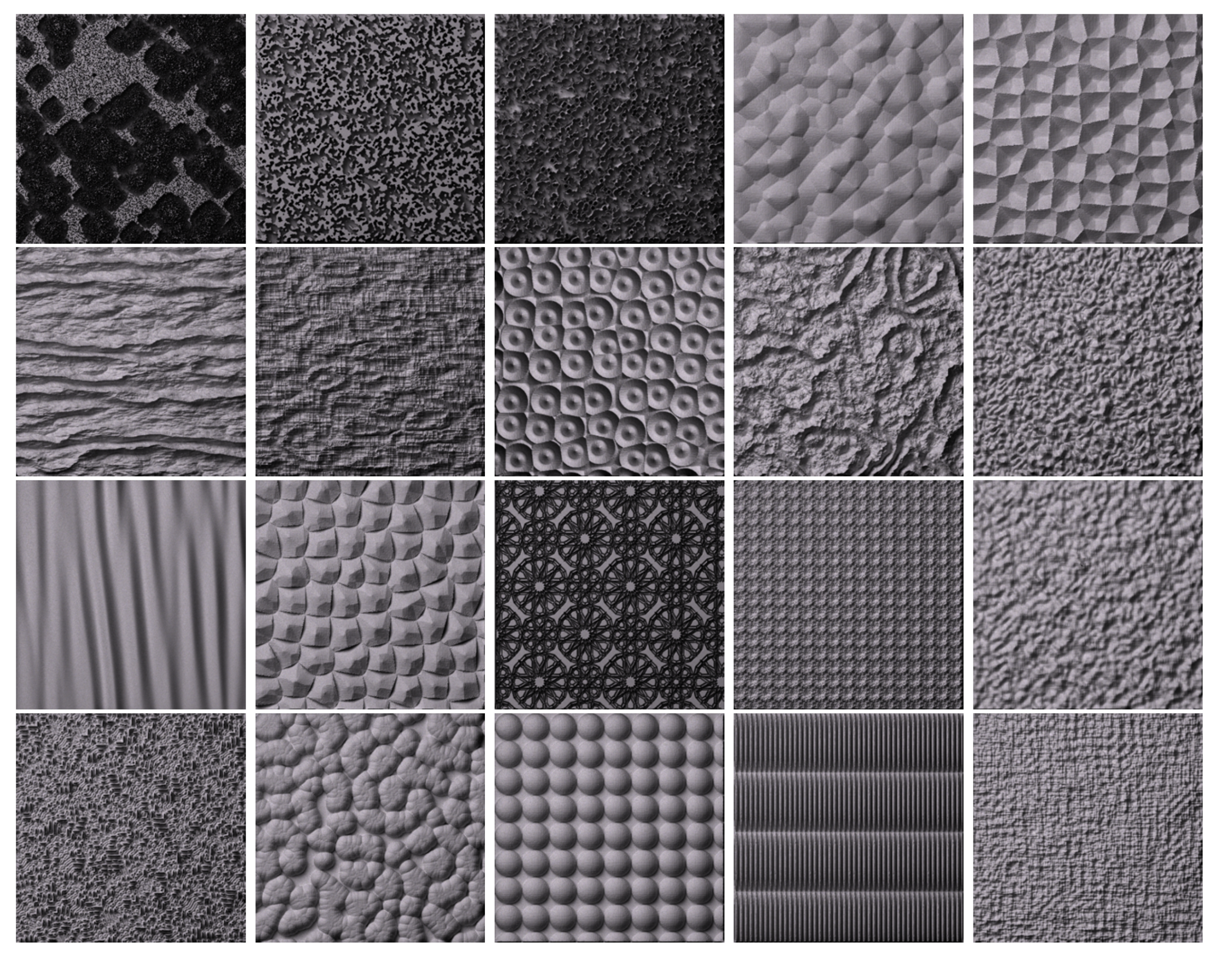
4.1. Result on Texture Data Sets

In this subsection, we introduce the experimental results obtained on the texture data sets.

4.1.1. Psychophysical Experiments

In this experiment, we used 450 texture images, which were generated by 23 procedural texture models (23 categories) [23,72]. As shown in Figure 1, we selected some example images randomly from this data set. The score of each perceptual feature is represented by 1 to 9. A ‘1’ indicates that the observer’s perception of the perceptual feature is weak, and a ‘9’ is very strong. The perceptual features were designed based on previous work on texture perception [17,19]. A total of 12 perceptive features were found to be the most important through a thorough analysis of the psychophysical test results. They were contrast, repetitiveness, granularity, randomness, roughness, density, direction, structural complexity, coarseness, regularity, orientation, and uniformity. Hence, each texture image is represented by a 12-dimensional vector, corresponding to the values of the 12 perceptual features (All data files are available at https://figshare.com/articles/dataset/procedural_textures/1289700, accessed on 31 December 2020).

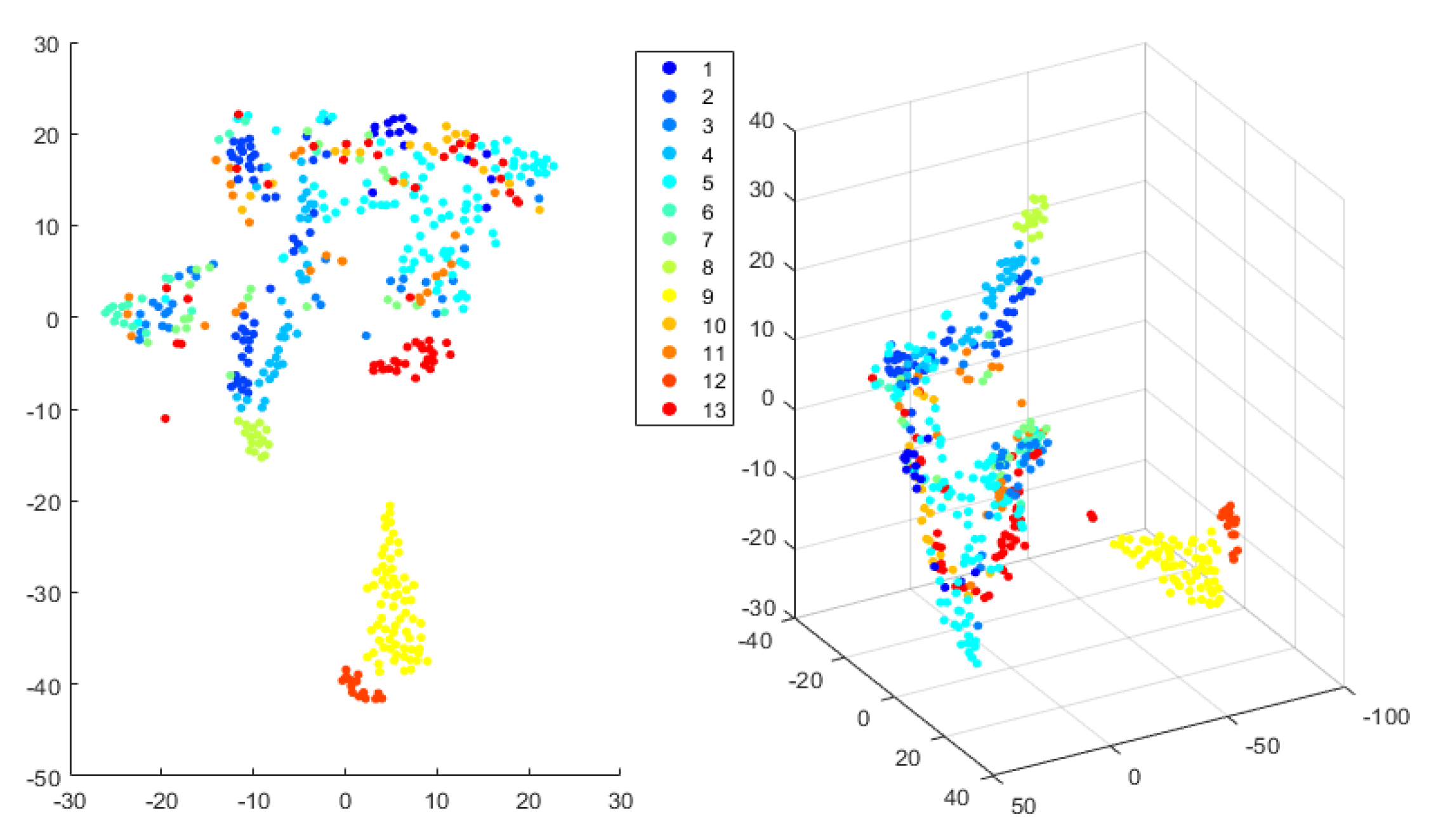
4.1.2. Visualization

To visualize the 12-dimensional perceptual features in 2D and 3D spaces, we used t-SNE to learn the low-dimensional embeddings of the original data. The learned results are shown in Figure 3. From the figure, we can see in the original data space that it is very challenging to distinguish the classes from each other, because different classes are heavily overlapped with each other.

Figure 4 shows two texture images; their appearances look very similar. However, they are generated from different procedural models, i.e., they belong to two different categories. The psychophysical test results show that the 12 perceptual features of the left image are (5.3, 6.05, 4.8, 3.35, 4.75, 5, 5.25, 3.65, 5, 5.3, 5.6, 6.7), and that of the right image are (5.65, 6.7, 4.75, 2.9, 4.3, 5.15, 4.65, 3.85, 4.4, 6.05, 5.35, 6.75). Due to the fact that even humans find it very difficult to distinguish them from each other, we considered combining data belonging to different classes but with similar appearance together. In this case, we obtained a 13-class problem. The new 2D and 3D embedding of the combined data are shown in Figure 5.

4.1.3. Classification Results

Both the original and combined texture perceptual data (12-dimensional perceptual features) were used to evaluate the ability of the feature learning models and the proposed deep architectures in processing texture perception features. Specifically, the classifier used in SDA was a support vector machine (SVM) with the radial basis function (RBF) kernel [73], and 5-fold cross validation was used to mean the accuracy of the experimental results. In particular, we tested the compared methods on different settings with respect to the dimensionality of the low-dimensional embeddings. Concretely, the dimensionality of the low-dimensional embeddings was set to 3 and 6, respectively. For concreteness, if the dimensionality of the embeddings was 3, an architecture

$$\begin{array}{c}\hfill 12D\frac{PCA}{}10D\frac{FL}{}8D\frac{FL}{}6D\frac{FL}{}5D\frac{FL}{}4D\frac{FL}{}3D\frac{SC}{}L.\end{array}$$

(15)

was used, while if the dimensionality of the embeddings was 6, an architecture

$$12D\frac{PCA}{}10D\frac{FL}{}8D\frac{FL}{}6D\frac{SC}{}L,$$

(16)

was applied. If the last feature learning module is nonlinear, we added a PCA layer to it, as mentioned in Section 3.3. Generally, the mapping modes of linear and nonlinear feature learning models were different. A projection matrix could be learned to perform feature mapping in linear feature learning models, whilst for nonlinear feature learning models, the three nearest neighbors of a test datum in the training data were used to estimate its low-dimensional representation. The final low-dimensional representations of the test data were obtained by learning layer by layer.

For MFA [40], the numbers of nearest neighbors for constructing the intrinsic graph and penalty graph were set to 5 and 15, respectively. For deep autoencoder (Autoencoder), as it is a classical deep learning method, we used it as the baseline. We set the layers of Autoencoder for the target spaces with dimensionality 3 and 6 as 12D-20D-8D-4D-3D and 12D-20D-11D-7D-6D. For the LeNet model, we used two convolutional layers and two fully connected layers without a pooling layer because of the lower dimension of texture data. The kernel size was set to $2\times 2$, the stride was set to 1, the number of nodes in the first fully connected layer was set to 100, the epoch was set to 4000, the initial learning rate was set to 0.001, and the momentum was set to 0.9. For the PCANet model, we used two PCA filter stages, one binary hashing stage, and one blockwise histogram. In PCANet, the filter size, the number of filters, and the block size were set to $k_1=k_2=3$, $L_1=L_2=2$, and $2\times 2$, respectively. For the learning rate policy, we used

$$r_i=r_0\times {(1+\gamma \times i)}^{-m},$$

(17)

where $r_i$ was the learning rate of the ith iteration, $r_0$ was the initial learning rate, $\gamma$ was set to 0.0001, and m was set to 0.75. Here, the compared deep learning models, i.e., Autoencoder, LeNet, and PCANet, have similar scales of parameters with SDA, while including both fully connected networks and CNNs. For other deep learning models, such as ResNet and ViT [31,35], although they are widely used in many applications, they have much more parameters than SDA. It is not fair to compare SDA with them. Hence, we do not consider them for the comparison with SDA in this experiment.

Table 1. Classification accuracy in the 6D space (before stretching) of the texture data set. “ORIG” represents the results obtained in the original data space. “shallow” denotes that algorithm only uses the single-layer feature learning models. ‘L’ represents the dimensionality of the stretched space. The best two results are highlighted with boldface.

Method	Shallow	Deep	$\mathit{L}=12$	$\mathit{L}=24$	$\mathit{L}=48$	$\mathit{L}=96$	$\mathit{L}=192$	$\mathit{L}=500$	$\mathit{L}=\mathit{\infty }$
ORIG	0.5524 ±0.2302	- -	- -	- -	- -	- -	- -	- -	- -
Autoencoder	- -	0.3984 ±0.1116	- -	- -	- -	- -	- -	- -	- -
LeNet	- -	0.4214 ±0.1008	- -	- -	- -	- -	- -	- -	- -
PCANet	- -	0.4691 ±0.0854	- -	- -	- -	- -	- -	- -	- -
PCA	0.4388 ±0.2178	0.4215 ±0.2408	0.5578 ±0.0617	0.5640 ±0.0264	0.6217 ±0.0673	0.6266 ±0.0649	0.6168 ±0.0609	0.6109 ±0.0562	0.4228 ±0.0365
PPCA	0.3226 ±0.1947	0.3115 ±0.0623	0.3215 ±0.0980	0.3885 ±0.0620	0.3730 ±0.0445	0.3966 ±0.0531	0.4175 ±0.1144	0.3829 ±0.0491	0.2404 ±0.0507
MDS	0.4365 ±0.1742	0.5406 ±0.0995	0.5386 ±0.0567	0.5684 ±0.0562	0.5758 ±0.0524	0.5875 ±0.0683	0.5619 ±0.0513	0.5660 ±0.0478	0.3966 ±0.0516
Sammon	0.5023 ±0.1964	0.5658 ±0.0543	0.5300 ±0.0567	0.5783 ±0.0597	0.5700 ±0.0439	0.5922 ±0.0710	0.5989 ±0.0734	0.5931 ±0.0636	0.4321 ±0.0586
SNE	0.4192 ±0.2409	0.5289 ±0.1371	0.5199 ±0.0435	0.5547 ±0.0617	0.5529 ±0.0537	0.5610 ±0.0581	0.5718 ±0.0610	0.5693 ±0.0576	0.4106 ±0.0720
MFA	0.5552 ±0.0622	0.5593 ±0.0798	0.5601 ±0.0712	0.5621 ±0.0734	0.5738 ±0.0671	0.5496 ±0.0446	0.5422 ±0.0495	0.5335 ±0.0527	0.3984 ±0.0540

and

Table 2. Classification accuracy in the 3D space of texture data set.

Method	Shallow	Deep	$\mathit{L}=12$	$\mathit{L}=24$	$\mathit{L}=48$	$\mathit{L}=96$	$\mathit{L}=192$	$\mathit{L}=500$	$\mathit{L}=\mathit{\infty }$
ORIG	0.5524 ±0.2302	- -	- -	- -	- -	- -	- -	- -	- -
Autoencoder	- -	0.4392 ±0.0982	- -	- -	- -	- -	- -	- -	- -
LeNet	- -	0.4214 ±0.1008	- -	- -	- -	- -	- -	- -	- -
PCANet	- -	0.4691 ±0.0854	- -	- -	- -	- -	- -	- -	- -
PCA	0.3982 ±0.0906	0.3667 ±0.0795	0.4596 ±0.0529	0.4575 ±0.0695	0.4765 ±0.0812	0.4836 ±0.0712	0.4624 ±0.0309	0.4882 ±0.0523	0.3638 ±0.0254
PPCA	0.4649 ±0.0703	0.4679 ±0.0577	0.5095 ±0.0619	0.5115 ±0.0678	0.5212 ±0.0652	0.5266 ±0.0573	0.5046 ±0.0601	0.5092 ±0.0851	0.3988 ±0.0807
MDS	0.4628 ±0.0724	0.4797 ±0.0954	0.4921 ±0.0514	0.5035 ±0.0424	0.5342 ±0.0614	0.5028 ±0.0640	0.4963 ±0.0661	0.5243 ±0.0586	0.3806 ±0.0494
Sammon	0.4698 ±0.0653	0.4791 ±0.0774	0.5245 ±0.0713	0.5245 ±0.0639	0.5088 ±0.0617	0.5056 ±0.0609	0.5153 ±0.0562	0.5007 ±0.0619	0.3852 ±0.0374
SNE	0.5531 ±0.0904	0.4683 ±0.0489	0.5160 ±0.0568	0.5028 ±0.0452	0.5248 ±0.0677	0.5631 ±0.0521	0.5039 ±0.0647	0.4915 ±0.0579	0.3843 ±0.0333
MFA	0.4601 ±0.0475	0.4634 ±0.0475	0.4689 ±0.0352	0.4712 ±0.0431	0.4856 ±0.0372	0.5012 ±0.0234	0.4765 ±0.0528	0.4712 ±0.0327	0.3834 ±0.0413

show the classification results obtained by the compared methods. Here, because LDA-based approaches performed much worse than others, the results obtained by them were not included. From Table 1 and Table 2, we can see that, firstly, both the feature learning models and SDA are effective for the visual texture perception problems; secondly, deep learning models perform better than or at least comparable with the compared feature learning models; and thirdly, SDA performs better than other stretching deep architectures, i.e., the previous Autoencoder, LeNet, and PCANet. In addition, we can find the best two stretching spaces, 48D and 96D, which donate more “winner” results than other spaces.

On the other hand, we can find that when we adopted the stretching strategy, SDA could achieve good performances in the 6D space using the deep architecture with stacked PCAs, while in the 3D space, the deep architecture with stacked SNEs performed better than other methods. This may be because that PCA is a linear model, while SNE is a nonlinear model. When the dimensionality of the target space is relatively high, linear models could achieve better performance; while the dimensionality of the target space is relatively low, nonlinear models could perform better. In the 6D space, with the stretching operation, the accuracy of the deep architectures with stacked PCAs and MDSs increased for $L<96$, those with stacked PPCAs, SNEs and Sammons increased for $L<192$, that with stacked MFAs increased for $L<48$, and all the methods achieved better performance than in the original 12D space. In the 3D space, we can obtain a similar conclusion as in the 6D space, and only the deep architectures with stacked SNEs were better than in the original data space when stretching in 3D space. These results sufficiently show that the stretching operation could improve the performance of deep architectures.

Figure 6 shows the classification results obtained by variants of SDA on the combined texture data. We chose the 6D space as the semantic space. Here, we can see two interesting points: the classification results in this space are better than in the original space using the deep architectures with stacked PCAs, PPCAs, MFAs, and the stretching operation; and not surprisingly, the deep architecture with stacked PCAs achieves the highest accuracy.

4.2. Experimental Results on Handwritten Text Data Sets

To evaluate the effectiveness of SDA in the applications of handwritten text recognition, we tested it on three data sets, i.e., handwritten digits data set USPS (http://www.gaussianprocess.org/gpml/data/, accessed on 31 December 2020), ancient Arabic documents data set Ibn Sina (http://www.causality.inf.ethz.ch/al_data/IBN_SINA.html, accessed on 31 December 2020) and English letter data set Letter (http://archive.ics.uci.edu/ml/, accessed on 31 December 2020). The classifier used in SDA were SVMs [73]. Both deep neural network models and shallow feature learning models were used to compare with SDA. For concreteness, PCA [24], PPCA [36], Sammon [37], SNE [38], MDS [39], LDA [25], MFA [40,41], and deep autoencoder (Autoencoder) [7] were used. The recognition results in the original space of data and that learned with and without stretching in SDA were all reported. Different values of L were tested for the stretching operation. For the parameter settings of the compared methods, we adopted the same as introduced in the above subsection.

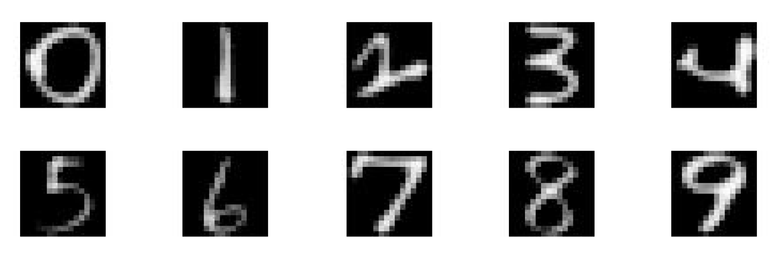
4.2.1. Results on the USPS Data Set

The USPS data set includes 10 classes of handwritten digits, with a dimensionality of 256. There are 7291 training samples and 2007 test samples. Figure 7 shows 10 images from each class of digits ‘0’ to ‘9’. On this data set, the structure of the Autoencoder was set to 256D-512D-256D-128D-64D-32D. For the LeNet model, we used two convolutional layers, two pooling layers, and two fully connected layers. The kernel size of convolutional layers and pooling layer was set to $2\times 2$, the stride was set to 1, the number of nodes of the first layer was set to 200, the epoch was set to 8000, the initial learning rate was set to 0.001, the learning rate policy was set as shown in Equation (17), and the momentum was set to 0.9. For the PCANet model, we also used two PCA filter stages, one binary hashing stage, and one blockwise histogram. Parameters in PCANet, the filter size, the number of filters, and the block size, were set to $k_1=k_2=3$, $L_1=L_2=4$, and $7\times 7$, respectively. The particle swarm optimization (PSO) method [74] was used to learn the parameter C in SVMs. If SDA was built using linear feature learning modules, the architecture was designed as

$$256D\frac{FL}{}128D\frac{FL}{}64D\frac{FL}{}32D\frac{SC}{}L,$$

(18)

where the feature learning modules were represented by ‘FL’, and the stretching operation was represented by ‘SC’. Note that when LDA was used to construct SDA, since the number of classes of the USPS data set was 10, the dimension of the learned subspace was set to 9. Since nonlinear feature learning models had no projection matrix, we used PCA on the last layer to perform stretching

$$256D\frac{FL}{}128D\frac{FL}{}64D\frac{FL}{}32D\frac{PCA}{}32D\frac{SC}{}L.$$

(19)

The classification results obtained by different models are shown in

Table 3. Classification accuracy on the USPS data set. “ORIG” represents the results obtained in the original data space. “shallow” denotes that the method is applied with only a single-layer feature learning model. ‘L’ represents the dimensionality of the stretched space. The best two results are highlighted in boldface.

Method	Shallow	Deep	$\mathit{L}=64$	$\mathit{L}=128$	$\mathit{L}=256$	$\mathit{L}=512$	$\mathit{L}=1000$	$\mathit{L}=\mathit{\infty }$
ORIG	0.8366	–	–	–	–	–	–	–
Autoencoder	–	0.9402	–	–	–	–	–	–
LeNet	–	0.8032	–	–	–	–	–	–
PCANet	–	0.9477	–	–	–	–	–	–
PCA	0.9402	0.9427	0.9472	0.9492	0.9507	0.9517	0.8829	0.8615
PPCA	0.9342	0.9372	0.9367	0.9382	0.9372	0.9342	0.8789	0.8645
Sammon	0.9292	0.9302	0.9318	0.9342	0.9372	0.9397	0.8894	0.8794
SNE	0.9312	0.9367	0.9372	0.9382	0.9397	0.9422	0.8869	0.8749
MDS	0.9278	0.9292	0.9307	0.9352	0.9367	0.9387	0.8914	0.8824
LDA(9D)	0.9243	0.9268	0.9292	0.9342	0.9312	0.9302	0.8969	0.8879
MFA	0.9392	0.9432	0.9412	0.9442	0.9457	0.9497	0.8929	0.8857

. We can easily see that SDA outperforms not only shallow feature learning models but also some deep neural networks. Moreover, stretching deep architectures can indeed improve classification accuracy, but it does not apply to all dimensions. For example, the classification accuracy decreases when L is very large or close to infinite.

From Table 3, we can see that the performances of the deep architectures with stacked PCAs, Sammons, SNEs, MDSs, and MFAs increase for $L<512$. Furthermore, the performances of that with stacked PPCAs and LDAs increases for $L<256$. In addition, the results achieved by linear methods are better than nonlinear methods. Finally, PCA- and MFA-based deep architectures achieve the highest classification accuracy on the USPS data set.

Figure 8 shows the effect of the stretching operation in SDA that is built upon PCAs. We can see that the accuracy increases first and then decreases with the increase in stretching dimension L, and the highest accuracy is obtained when stretching to the 682 dimension.

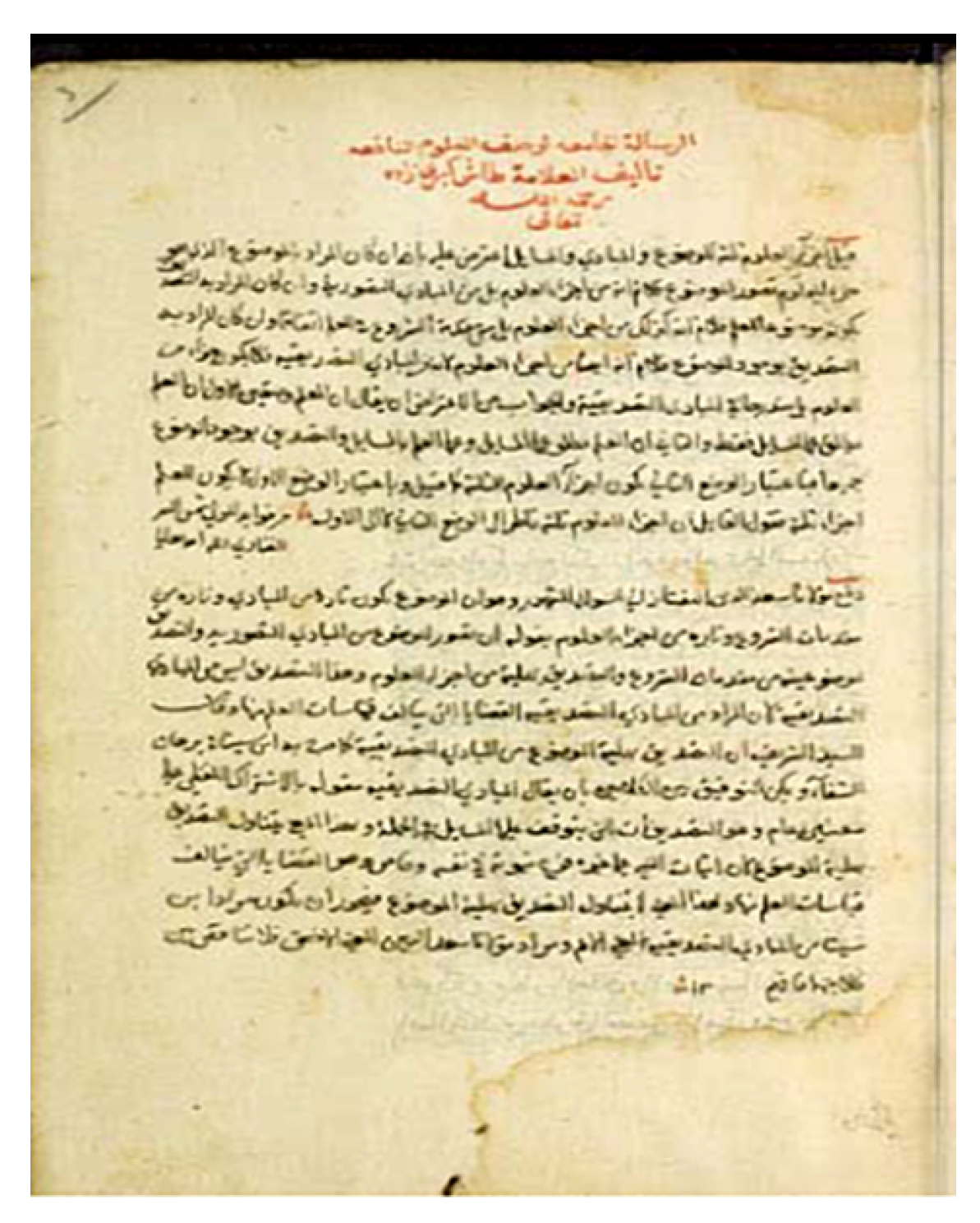
4.2.2. Results on the Ibn Sina Data Set

Figure 9 shows one page of the Ibn Sina ancient Arabic document images. We can easily see that the recognition of ancient Arabic words is more challenging than handwritten digit recognition. For this data set, 50 pages of the manuscript were used for training (including 17,543 training samples) and 10 pages for testing (including 3125 test samples) from 174 classes. The dimensionality of the Ibn Sina data was 200. In this experiment, for Autoencoder, the layers were set to 200D-400D-200D-50D-25D. The parameters of the LeNet model and PCANet were the same as the experiment of USPS, except that the epoch of LeNet was set to 40,000. The parameter C of SVMs was set to 15. Empirically, we designed a four-layer deep architecture for SDA using linear feature learning modules

$$200D\frac{FL}{}100D\frac{FL}{}50D\frac{FL}{}25D\frac{SC}{}L.$$

(20)

The architecture of SDA using nonlinear feature learning modules was set as follows

$$200D\frac{FL}{}100D\frac{FL}{}50D\frac{FL}{}25D\frac{PCA}{}25D\frac{SC}{}L.$$

(21)

Table 4. Classification accuracy on the Ibn Sina data set.

Method	Shallow	Deep	$\mathit{L}=100$	$\mathit{L}=200$	$\mathit{L}=500$	$\mathit{L}=2000$	$\mathit{L}=\mathit{\infty }$
ORIG	0.9274	–	–	–	–	–	–
Autoencoder	–	0.9334	–	–	–	–	–
LeNet	–	0.8195	–	–	–	–	–
PCANet	–	0.8995	–	–	–	–	–
PCA	0.9056	0.9184	0.9258	0.9328	0.9453	0.9478	0.9002
PPCA	0.9232	0.9258	0.9274	0.9347	0.9363	0.9369	0.9011
Sammon	0.9110	0.9197	0.9235	0.9274	0.9315	0.9254	0.9082
SNE	0.9034	0.9168	0.9197	0.9235	0.9261	0.9242	0.9011
MDS	0.9200	0.9219	0.9286	0.9264	0.9267	0.9276	0.9058
LDA	0.9258	0.9274	0.9389	0.9395	0.9384	0.9389	0.9014
MFA	0.9263	0.9316	0.9359	0.9440	0.9466	0.9491	0.9107

shows the classification results on the Ibn Sina data set. We can see that the accuracy is improved when we use the stretching operation. Furthermore, the accuracy is higher than that in the original data in most cases when the feature dimension is stretched to 200 (original dimensionality). The result of the deep architecture with stacked SNEs increases when $L<500$, and others increase when $L<2000$. In addition, same as on the USPS data set, the deep architectures with stacked MFAs and PCAs achieve the best results.

4.2.3. Results on the Letter Data Set

The Letter data set includes 20,000 samples from 26 classes. We used 16,000 data for training and 4000 data for testing. In our experiments, the layers of Autoencoder were set to 16D-32D-16D-15D-14D. For the LeNet model, we used two convolutional layers and two fully connected layers without a pooling layer. The kernel size was set to $2\times 2$, the stride was set to 1, the number of nodes of the first fully connected layer was set to 64, the epoch was set to 4000, the initial learning rate was set to 0.001, the learning rate policy was set as shown in Equation (17), and the momentum was set to 0.9. For PCANet, we used two PCA filter stages, one binary hashing stage, and one blockwise histogram. In PCANet, the filter size, the number of filters, and the block size were set to $k_1=k_2=3$, $L_1=L_2=4$, and $4\times 4$, respectively. The parameter C of the SVM classifier was set to 35. Due to the dimensionality of the data being less than other data set, we only use a two-layer structure. For linear feature learning modules, the architecture we designed was as follows:

$$16D\frac{FL}{}15D\frac{FL}{}14D\frac{SC}{}L.$$

(22)

For nonlinear feature learning modules, the architecture was

$$16D\frac{FL}{}15D\frac{FL}{}14D\frac{PCA}{}14D\frac{SC}{}L.$$

(23)

Table 5. Classification accuracy on the Letter data set.

Method	Shallow	Deep	$\mathit{L}=50$	$\mathit{L}=200$	$\mathit{L}=500$	$\mathit{L}=1000$	$\mathit{L}=\mathit{\infty }$
ORIG	0.8635	–	–	–	–	–	–
Autoencoder	–	0.8823	–	–	–	–	–
LeNet	–	0.6070	–	–	–	–	–
PCANet	–	0.5823	–	–	–	–	–
PCA	0.8565	0.8600	0.8613	0.8675	0.8713	0.8680	0.8613
PPCA	0.9610	0.9690	0.9703	0.9680	0.9430	0.9285	0.8988
Sammon	0.8233	0.8340	0.8388	0.8413	0.8345	0.8313	0.8255
SNE	0.7715	0.7750	0.7845	0.7893	0.8023	0.7895	0.7760
MDS	0.8673	0.8723	0.8750	0.8795	0.8770	0.8653	0.8620
LDA	0.9630	0.9688	0.9693	0.9720	0.9730	0.9713	0.9610
MFA	0.9670	0.9690	0.9713	0.9735	0.9758	0.9680	0.9520

shows the classification results on the Letter data set. We can obtain a similar conclusion as on the USPS and the Ibn Sina data set. The results of LeNet and PCANet are especially poor. The reason is that the dimensionality of the Letter data is low, and CNNs are not suited to it. In addition, we can find that the deep architectures with stacked PPCAs, LDAs, and MFAs achieve the best results. By analyzing the obtained results on these three data sets (USPS, Ibn Sina, and Letter), we can basically obtain the consistent conclusion that if we stretch the deep architecture to an infinite length, the original features might be submerged in the noise. On the contrary, if we set the length suitably, the new features will be adapted to the classifier and obtain better results than without stretching.

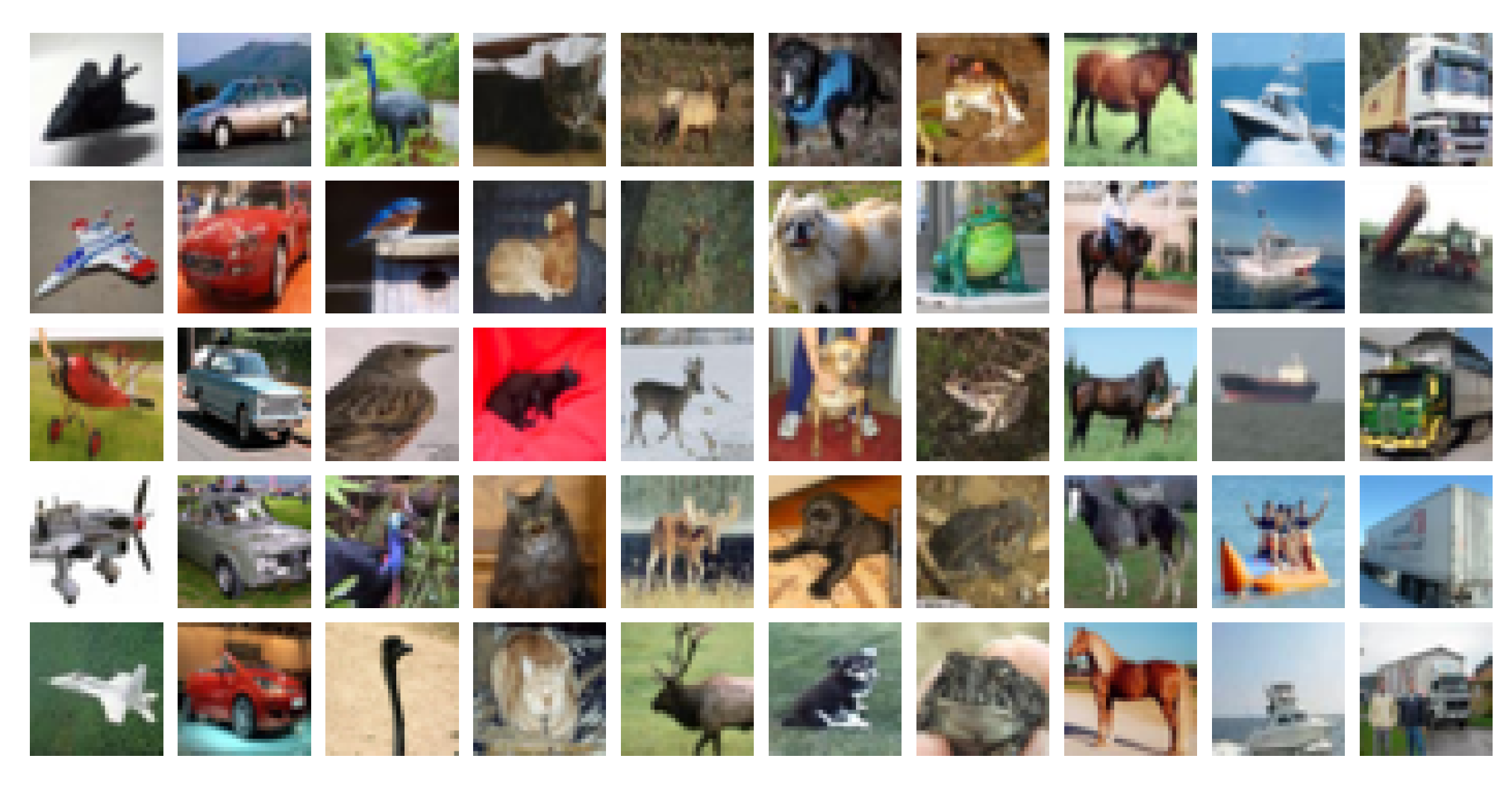
4.3. Classification of the Cifar-10 Data Set

The CIFAR-10 data set is a relatively large data set, which consists of 60,000 $32\times 32$ color images in 10 classes, with 6000 images per class. There are 50,000 training images and 10,000 test images. Figure 10 shows some examples of the CIFAR-10 data set from 10 categories. For the purpose of reducing computational cost, we attempted to create a compact representation of the data using an efficient local binary patterns algorithm. As a result, the representation of dimensionality 36 and 256 were adopted, and the data were normalized to [0, 1] as well. For SDA, the layers were set to 36D-18D-9D and 256D-128D-64D-32D. For Autoencoder, The layers were set to 36D-72D-36D-18D-9D and 256D-512D-126D-128D-64D-32D. For the LeNet model, we used two convolutional layers and two fully connected layers without a pooling layer. The kernel size was set to $2\times 2$, the stride was set to 1, the number of nodes of the first fully connected layer was set to 64, the epoch was set to 4000, the initial learning rate was set to 0.01, the learning rate policy was set as shown in Equation (17), and the momentum was set to 0.9. For PCANet, we used two PCA filter stages, one binary hashing stage, and one blockwise histogram. In the PCANet, the filter size, the number of filters, and the block size were set to $k_1=k_2=3$, $L_1=L_2=4$, and $7\times 7$, respectively. To further demonstrate the performance of SDA, we compared SDA with the classical CNN model AlexNet [29] on CIFAR-10 (256) data set. All the parameters of AlexNet are the same as [29] except for the kernel size of convolutional layers and pooling layers. We set the kernel size to $2\times 2$, and the stride was set to 1. The parameter C of the SVM classifier was set to the default value.

Table 6. Classification accuracy obtained on the CIFAR-10 (36) set.

Method	Shallow	Deep	$\mathit{L}=36$	$\mathit{L}=72$	$\mathit{L}=200$	$\mathit{L}=500$	$\mathit{L}=\mathit{\infty }$
ORIG	0.3225	–	–	–	–	–	–
Autoencoder	–	0.3521	–	–	–	–	–
LeNet	–	0.3256	–	–	–	–	–
PCANet	–	0.2569	–	–	–	–	–
PCA	0.3379	0.3385	0.3398	0.3439	0.3489	0.3478	0.3358
PPCA	0.3385	0.3374	0.3385	0.3395	0.3402	0.3411	0.3388
Sammon	0.3278	0.3285	0.3312	0.3356	0.3389	0.3378	0.3314
SNE	0.3355	0.3387	0.3397	0.3425	0.3438	0.3441	0.3322
MDS	0.3311	0.3335	0.3356	0.3397	0.3415	0.3401	0.3325
LDA	0.3178	0.3211	0.3256	0.3298	0.3301	0.3341	0.3211
MFA	0.3401	0.3438	0.3479	0.3511	0.3546	0.3536	0.3359

and

Table 7. Classification accuracy obtained on the CIFAR-10 (256) set.

Method	Shallow	Deep	$\mathit{L}=64$	$\mathit{L}=128$	$\mathit{L}=256$	$\mathit{L}=500$	$\mathit{L}=1000$	$\mathit{L}=\mathit{\infty }$
ORIG	0.3218	–	–	–	–	–	–	–
Autoencoder	–	0.3448	–	–	–	–	–	–
AlexNet	–	0.3356	–	–	–	–	–	–
LeNet	–	0.3221	–	–	–	–	–	–
PCANet	–	0.2569	–	–	–	–	–	–
PCA	0.3378	0.3382	0.3398	0.3405	0.3451	0.3442	0.3435	0.3382
PPCA	0.3358	0.3389	0.3415	0.3426	0.3456	0.3458	0.3425	0.3378
Sammon	0.3314	0.3356	0.3389	0.3436	0.3441	0.3432	0.3402	0.3347
SNE	0.3312	0.3341	0.3375	0.3389	0.3401	0.3412	0.3385	0.3289
MDS	0.3345	0.3358	0.3425	0.3435	0.3432	0.3438	0.3389	0.3322
LDA	0.3341	0.3358	0.3372	0.3396	0.3411	0.3415	0.3401	0.3356
MFA	0.3402	0.3414	0.3456	0.3472	0.3488	0.3452	0.3402	0.3399

show the experimental results of the CIFAR-10 data set. We can basically achieve the same conclusion as previous experiments. In addition, SDA outperforms AlexNet, LeNet, and PCANet in these experiments. The deep architecture with stacked MFAs achieves the best results. From these experiments, we can obtain that SDA works well in the relatively large-scale data set for semantic representation learning.

4.4. Improving the Effectiveness of CNNs

To demonstrate that SDA can improve the effectiveness of CNNs on image classification tasks, we built a deep CNN model with its structure shown in

Table 8. Structure of our baseline convolutional neural network.

Layer	Output Shape	Kernal Size
Conv_1	(32, 32, 32)	(3 × 3)
Activation_1 (ReLU)	(32, 32, 32)	–
Max Pooling_1	(16, 16, 32)	(2 × 2)
Conv_2	(16, 16, 64)	(3 × 3)
Activation_2 (ReLU)	(16, 16, 64)	–
Max pooling_2	(8, 8, 64)	(2 × 2)
Flatten_1	(4096, 1)	–
Dense_1	(512, 1)	–
Dense_2	(256, 1)	–
Dense_3 (Softmax)	(10, 1)	–

and trained this CNN model on the original CIFAR-10 data set. For this CNN model, we used two convolutional layers, all of which used max pooling, and two fully connected layers, where the numbers of nodes were set to 512 and 256, respectively. The RMSProp optimizer was used to perform optimization of the parameters. For SDA, the input features were that output from the second fully connected layer of the CNN model. In addition, the layers were set to 256D-200D-150D-100D-50D. Particularly, PCA, LDA, and MDS were selected to construct the SDA architecture and perform comparisons with the baseline CNN model.

Table 9. Classification accuracy obtained on the CIFAR-10 data set.

Method	Deep	$\mathit{L}=100$	$\mathit{L}=200$	$\mathit{L}=500$	$\mathit{L}=1000$	$\mathit{L}=\mathit{\infty }$
Baseline CNN	0.7158	–	–	–	–	–
PCA	0.7347	0.7348	0.7364	0.7345	0.7320	0.7205
LDA	0.7208	0.7241	0.7198	0.6098	0.6124	0.6972
MDS	0.7320	0.7340	0.7325	0.7321	0.7319	0.7193

shows that SDA with stacked PCAs achieves the best results among the compared models. Hence, we can easily conclude that SDA can make full use of the fully connected layer of the CNNs and improve their classification accuracy. In particular, for large image data sets or complex image classification problems, we can apply CNNs or ViT to extract features for SDA, or integrate SDA with CNNs and ViT to perform image classification. In this case, SDA may improve the performance of the original CNNs or ViT model.

4.5. Evaluation of the Number of Feature Learning Layers

To evaluate the number of feature learning layers, we designed the experiments on handwritten text data sets. We set the number of hidden layers from one to seven layers, and the parameters were the same as in previous experiments. For the last stretching layers, we set L as the same as the previous experiments that achieved the best results. Furthermore, all SDAs were based on stacking MFAs.

Figure 11 shows the results on the different number of feature learning layers. We can see that three to five feature learning layers obtain the best results. In addition, when the number of feature learning layers are less than 3, the results increase along with the number of feature learning layers. Then, the results will decrease with the increase in the number of feature learning layers.

5. Conclusions

In this paper, we proposed a novel deep learning method called SDA for semantic representation learning. SDA is constructed using stacked shallow feature learning modules. The stretching technique is applied to improve the learning performance of SDA. Extensive experiments on visual texture perception and image classification problems demonstrate that, in most cases, SDA greatly improves both traditional feature learning and deep learning models. In some cases, SDA can also improve the accuracy of CNNs. For future work, we plan to adopt some other techniques to enhance SDA, such as supervised fine-tuning and dropout regularization. It is expected that these techniques can greatly improve SDA in many object recognition tasks. Specifically, when the training data are limited, the regularization techniques can, to some extent, handle the overfitting problem. Moreover, we would like to extend the applications of SDA to real-world open sets, which are much more challenging than the tested closed sets in this paper.

References

1. Chen, K.; Salman, A. Learning Speaker-Specific Characteristics with a Deep Neural Architecture. Neural Netw. IEEE Trans. 2011, 22, 1744–1756. [Google Scholar] [CrossRef]
2. Stuhlsatz, A.; Lippel, J.; Zielke, T. Feature Extraction with Deep Neural Networks by a Generalized Discriminant Analysis. Neural Netw. Learn. Syst. IEEE Trans. 2012, 23, 596–608. [Google Scholar] [CrossRef]
3. Yuan, M.; Tang, H.; Li, H. Real-Time Keypoint Recognition Using Restricted Boltzmann Machine. Neural Netw. Learn. Syst. IEEE Trans. 2014, 25, 2119–2126. [Google Scholar] [CrossRef]
4. Bengio, Y.; Courville, A.; Vincent, P. Representation Learning: A Review and New Perspectives. Pattern Anal. Mach. Intell. IEEE Trans. 2013, 35, 1798–1828. [Google Scholar] [CrossRef] [PubMed] [Green Version]
5. Deerwester, S.; Dumais, S.; Landauer, T.; Furnas, G.; Harshman, R. Indexing by Latent Semantic Analysis. JASIS 1990, 41, 391–407. [Google Scholar] [CrossRef]
6. Landauer, T.; Foltz, P.; Laham, D. An Introduction to Latent Semantic Analysis. Discourse Process. 1998, 25, 259–284. [Google Scholar] [CrossRef]
7. Hinton, G.; Salakhutdinov, R. Reducing the Dimensionality of Data with Neural Networks. Science 2006, 313, 504–507. [Google Scholar] [CrossRef] [PubMed] [Green Version]
8. Ainsworth, S. DeFT: A Conceptual Framework for Considering Learning with Multiple Representations. Learn. Instr. 2006, 16, 183–198. [Google Scholar] [CrossRef]
9. Bengio, Y. Learning Deep Architectures for AI. Found. Trends Mach. Learn. 2009, 2, 1–127. [Google Scholar] [CrossRef]
10. Lee, H.; Grosse, R.; Ranganath, R.; Ng, A. Convolutional Deep Belief Networks for Scalable Unsupervised Learning of Hierarchical Representations. In Proceedings of the ICML, Montreal, QC, Canada, 14–18 June 2009; ACM: New York, NY, USA, 2009; pp. 609–616. [Google Scholar]
11. Xiao, M.; Guo, Y. A Novel Two-Step Method for Cross Language Representation Learning. In Proceedings of the NIPS, Lake Tahoe, NY, USA, 5–10 December 2013; pp. 1259–1267. [Google Scholar]
12. Huang, P.S.; He, X.; Gao, J.; Deng, L.; Acero, A.; Heck, L. Learning Deep Structured Semantic Models for Web Search Using Clickthrough Data. In Proceedings of the CIKM, San Francisco, CA, USA, 27 October–1 November 2013; ACM: New York, NY, USA, 2013; pp. 2333–2338. [Google Scholar]
13. Shen, Y.; He, X.; Gao, J.; Deng, L.; Mesnil, G. Learning Semantic Representations Using Convolutional Neural Networks for Web Search. In Proceedings of the WWW, Seoul, Republic of Korea, 7–11 April 2014; pp. 373–374. [Google Scholar]
14. Oveis, A.H.; Giusti, E.; Ghio, S.; Martorella, M. A Survey on the Applications of Convolutional Neural Networks for Synthetic Aperture Radar: Recent Advances. IEEE Aerosp. Electron. Syst. Mag. 2022, 37, 18–42. [Google Scholar] [CrossRef]
15. Landy, M.; Graham, N. Visual Perception of Texture. In Proceedings of the Visual Neurosciences; MIT Press: Cambridge, MA, USA, 2004; pp. 1106–1118. [Google Scholar]
16. Heeger, D.; Bergen, J. Pyramid-based Texture Analysis/Synthesis. In Proceedings of the SIGGRAPH, Los Angeles, CA, USA, 6–11 August 1995; ACM: New York, NY, USA, 1995; pp. 229–238. [Google Scholar]
17. Rao, A.; Lohse, G. Towards a Texture Naming System: Identifying Relevant Dimensions of Texture. Vis. Res. 1996, 36, 1649–1669. [Google Scholar]
18. Wolfson, S.; Landy, M. Examining Edge- and Region-based Texture Mechanisms. Vis. Res. 1998, 38, 439–446. [Google Scholar] [CrossRef] [PubMed] [Green Version]
19. Gurnsey, R.; Fleet, D. Texture Space. Vis. Res. 2001, 41, 745–757. [Google Scholar] [CrossRef] [PubMed] [Green Version]
20. Kingdom, F.; Hayes, A.; Field, D. Sensitivity to Contrast Histogram Differences in Synthetic Wavelet-Textures. Vis. Res. 2001, 41, 585–598. [Google Scholar] [CrossRef] [PubMed] [Green Version]
21. Durgin, F. Texture Contrast Aftereffects Are Monocular, Texture Density Aftereffects Are Binocular. Vis. Res. 2001, 41, 2619–2630. [Google Scholar] [CrossRef] [PubMed] [Green Version]
22. Zheng, Y.; Zhong, G.; Liu, J.; Cai, X.; Dong, J. Visual Texture Perception with Feature Learning Models and Deep Architectures. In Pattern Recognition, Proceedings of the 6th Chinese Conference, CCPR 2014, Changsha, China, 17–19 November 2014; Springer: Berlin/Heidelberg, Germany, 2014; pp. 401–410. [Google Scholar]
23. Liu, J.; Dong, J.; Cai, X.; Q, L.; Chantler, M. Visual Perception of Procedural Textures: Identifying Perceptual Dimensions and Predicting Generation Models. PLoS ONE 2015, 10, e0130335. [Google Scholar] [CrossRef] [PubMed] [Green Version]
24. Jolliffe, I. Principal Component Analysis, 2nd ed.; Springer: Berlin/Heidelberg, Germany, 2002. [Google Scholar]
25. Fisher, R. The Use of Multiple Measurements in Taxonomic Problems. Ann. Eugen. 1936, 7, 179–188. [Google Scholar] [CrossRef]
26. van der Maaten, L.; Postma, E.; van den Herik, H. Dimensionality Reduction: A Comparative Review. J. Mach. Learn. Res. 2009, 10, 66–71. [Google Scholar]
27. van der Maaten, L. An Introduction to Dimensionality Reduction Using Matlab. Report 2007, 1201, 62. [Google Scholar]
28. Salakhutdinov, R.; Hinton, G. Deep Boltzmann Machines. In Proceedings of the AISTATS, Clearwater, FL, USA, 16–19 April 2009; pp. 448–455. [Google Scholar]
29. Krizhevsky, A.; Sutskever, I.; Hinton, G. ImageNet Classification with Deep Convolutional Neural Networks. In Proceedings of the NIPS, Lake Tahoe, NV, USA, 3–6 December 2012; pp. 1106–1114. [Google Scholar]
30. Yin, F.; Wang, Q.F.; Zhang, X.Y.; Liu, C.L. ICDAR 2013 Chinese Handwriting Recognition Competition. In Proceedings of the ICDAR, Washington, DC, USA, 25–28 August 2013; pp. 1464–1470. [Google Scholar]
31. He, K.; Zhang, X.; Ren, S.; Sun, J. Deep Residual Learning for Image Recognition. arXiv 2015, arXiv:1512.03385. [Google Scholar]
32. Kattenborn, T.; Leitloff, J.; Schiefer, F.; Hinz, S. Review on Convolutional Neural Networks (CNN) in vegetation remote sensing. ISPRS J. Photogramm. Remote Sens. 2021, 173, 24–49. [Google Scholar] [CrossRef]
33. Yuan, Y.; Wang, L.N.; Zhong, G.; Gao, W.; Jiao, W.; Dong, J.; Shen, B.; Xia, D.; Xiang, W. Adaptive Gabor Convolutional Networks. Pattern Recognit. 2022, 124, 108495. [Google Scholar] [CrossRef]
34. Niu, Z.; Zhong, G.; Yu, H. A Review on the Attention Mechanism of Deep Learning. Neurocomputing 2021, 452, 48–62. [Google Scholar] [CrossRef]
35. Han, K.; Wang, Y.; Chen, H.; Chen, X.; Guo, J.; Liu, Z.; Tang, Y.; Xiao, A.; Xu, C.; Xu, Y.; et al. A Survey on Vision Transformer. IEEE Trans. Pattern Anal. Mach. Intell. 2022, 45, 87–110. [Google Scholar] [CrossRef] [PubMed]
36. Tipping, M.; Bishop, C. Probabilistic Principal Component Analysis. J. R. Stat. Soc. Ser. B (Stat. Methodol.) 1999, 61, 611–622. [Google Scholar] [CrossRef] [Green Version]
37. Sammon, J. A Nonlinear Mapping for Data Structure Analysis. IEEE Trans. Comput. 1969, 18, 401–409. [Google Scholar] [CrossRef]
38. Hinton, G.; Roweis, S. Stochastic Neighbor Embedding. In Proceedings of the NIPS, Vancouver, BC, Canada, 9–14 December 2002; Volume 2, pp. 833–840. [Google Scholar]
39. Kruskal, J.; Wish, M. Multidimensional Scaling; Sage: New York, NY, USA, 1978; Volume 11. [Google Scholar]
40. Yan, S.; Xu, D.; Zhang, B.; Zhang, H.J.; Yang, Q.; Lin, S. Graph Embedding and Extensions: A General Framework for Dimensionality Reduction. Pattern Anal. Mach. Intell. IEEE Trans. 2007, 29, 40–51. [Google Scholar] [CrossRef] [Green Version]
41. Zhong, G.; Chherawala, Y.; Cheriet, M. An Empirical Evaluation of Supervised Dimensionality Reduction for Recognition. In Proceedings of the ICDAR, Washington, DC, USA, 25–28 August 2013; pp. 1315–1319. [Google Scholar]
42. Pandey, G.; Dukkipati, A. Learning by Stretching Deep Networks. In Proceedings of the ICML, Beijing, China, 21–26 June 2014; pp. 1719–1727. [Google Scholar]
43. Zheng, Y.; Cai, Y.; Zhong, G.; Chherawala, Y.; Shi, Y.; Dong, J. Stretching Deep Architectures for Text Recognition. In Proceedings of the ICDAR, Tunis, Tunisia, 23–26 August 2015; pp. 236–240. [Google Scholar]
44. Ranzato, M.; Boureau, Y.; LeCun, Y. Sparse Feature Learning for Deep Belief Networks. In Proceedings of the NIPS, Vancouver, BC, Canada, 3–6 December 2007; pp. 1185–1192. [Google Scholar]
45. Lee, H.; Pham, P.; Largman, Y.; Ng, A. Unsupervised Feature Learning for Audio Classification Using Convolutional Deep Belief Networks. In Proceedings of the NIPS, Vancouver, BC, Canada, 7–10 December 2009; pp. 1096–1104. [Google Scholar]
46. LeCun, Y.; Bottou, L.; Bengio, Y.; Haffner, P. Gradient-Based Learning Applied to Document Recognition. Proc. IEEE 1998, 86, 2278–2324. [Google Scholar] [CrossRef] [Green Version]
47. Chan, T.H.; Jia, K.; Gao, S.; Lu, J.; Zeng, Z.; Ma, Y. PCANet: A Simple Deep Learning Baseline for Image Classification? Image Process. IEEE Trans. 2015, 24, 5017–5032. [Google Scholar] [CrossRef] [Green Version]
48. Vincent, P.; Larochelle, H.; Lajoie, I.; Bengio, Y.; Manzagol, P.A. Stacked Denoising Autoencoders: Learning Useful Representations in a Deep Network with a Local Denoising Criterion. J. Mach. Learn. Res. 2010, 11, 3371–3408. [Google Scholar]
49. Lin, M.; Chen, Q.; Yan, S. Network In Network. arXiv 2013, arXiv:1312.4400. [Google Scholar]
50. Julesz, B. Experiments in the visual perception of texture. Sci. Am. 1975, 232, 34–43. [Google Scholar] [CrossRef]
51. Julesz, B. Textons, the elements of texture perception, and their interactions. Nature 1981, 290, 91–97. [Google Scholar] [CrossRef] [PubMed]
52. Yu, Y.F.; Ren, C.X.; Dai, D.Q.; Huang, K.K. Kernel Embedding Multiorientation Local Pattern for Image Representation. IEEE Trans. Cybern. 2017, 48, 1124–1135. [Google Scholar] [CrossRef] [PubMed]
53. Ji, L.; Ren, Y.; Liu, G.; Pu, X. Training-Based Gradient LBP Feature Models for Multiresolution Texture Classification. IEEE Trans. Cybern. 2017, 48, 2683–2696. [Google Scholar] [CrossRef] [PubMed]
54. Graves, A.; Liwicki, M.; Fernandez, S.; Bertolami, R.; Bunke, H.; Schmidhuber, J. A Novel Connectionist System for Unconstrained Handwriting Recognition. Pattern Anal. Mach. Intell. IEEE Trans. 2009, 31, 855–868. [Google Scholar] [CrossRef] [Green Version]
55. Graves, A.; Schmidhuber, J. Offline Handwriting Recognition with Multidimensional Recurrent Neural Networks. In Proceedings of the NIPS, Vancouver, BC, Canada, 7–10 December 2009; pp. 545–552. [Google Scholar]
56. Graves, A. Generating Sequences with Recurrent Neural Networks. arXiv 2013, arXiv:1308.0850. [Google Scholar]
57. Liu, C.L.; Yin, F.; Wang, D.H.; Wang, Q.F. Online and Offline Handwritten Chinese Character Recognition: Benchmarking on New Databases. Pattern Recognit. 2013, 46, 155–162. [Google Scholar] [CrossRef]
58. Zeiler, M.; Fergus, R. Visualizing and Understanding Convolutional Networks. In Proceedings of the ECCV, Zurich, Switzerland, 6–12 September 2014; pp. 818–833. [Google Scholar]
59. Szegedy, C.; Liu, W.; Jia, Y.; Sermanet, P.; Reed, S.; Anguelov, D.; Erhan, D.; Vanhoucke, V.; Rabinovich, A. Going Deeper with Convolutions. In Proceedings of the CVPR, Boston, MA, USA, 7–12 June 2015; pp. 1–9. [Google Scholar]
60. Du, B.; Xiong, W.; Wu, J.; Zhang, L.; Zhang, L.; Tao, D. Stacked Convolutional Denoising Auto-Encoders for Feature Representation. IEEE Trans. Cybern. 2017, 47, 1017–1027. [Google Scholar] [CrossRef]
61. Qiao, H.; Li, Y.; Li, F.; Xi, X.; Wu, W. Biologically Inspired Model for Visual Cognition Achieving Unsupervised Episodic and Semantic Feature Learning. IEEE Trans. Cybern. 2016, 46, 2335–2347. [Google Scholar] [CrossRef] [PubMed]
62. Gama, J.; Brazdil, P. Cascade Generalization. Mach. Learn. 2000, 41, 315–343. [Google Scholar] [CrossRef]
63. Zhao, H.; Ram, S. Constrained Cascade Generalization of Decision Trees. Knowl. Data Eng. IEEE Trans. 2004, 16, 727–739. [Google Scholar] [CrossRef]
64. Viola, P.; Jones, M. Robust Real-time Object Detection. Int. J. Comput. Vis. 2001, 4. [Google Scholar]
65. Minguillón, J. On Cascading Small Decision Trees. Ph.D. Thesis, Universitat Autònoma de Barcelona, Barcelona, Spain, 2002. [Google Scholar]
66. Pang, Y.; Cao, J.; Li, X. Cascade Learning by Optimally Partitioning. IEEE Trans. Cybern. 2017, 47, 4148–4161. [Google Scholar] [CrossRef] [Green Version]
67. Zhang, Z.; Zha, H. Principal Manifolds and Nonlinear Dimensionality Reduction via Tangent Space Alignment. SIAM J. Sci. Comput. 2004, 26, 313–338. [Google Scholar] [CrossRef] [Green Version]
68. Zhong, G.; Li, W.J.; Yeung, D.Y.; Hou, X.; Liu, C.L. Gaussian Process Latent Random Field. In Proceedings of the AAAI, Atlanta, GA, USA, 11–15 July 2010. [Google Scholar]
69. Zhong, G.; Liu, C.L. Error-Correcting Output Codes Based Ensemble Feature Extraction. Pattern Recognit. 2013, 46, 1091–1100. [Google Scholar] [CrossRef]
70. Zhong, G.; Cheriet, M. Large Margin Low Rank Tensor Analysis. Neural Comput. 2014, 26, 761–780. [Google Scholar] [CrossRef] [Green Version]
71. Cho, Y.; Saul, L. Large-Margin Classification in Infinite Neural Networks. Neural Comput. 2010, 22, 2678–2697. [Google Scholar] [CrossRef] [Green Version]
72. Liu, J.; Dong, J.; Qi, L.; Chantler, M. Identifying Perceptual Features of Procedural Textures. In Proceedings of the ECVP, Bremen, Germany, 25–29 August 2013. [Google Scholar]
73. Chang, C.C.; Lin, C.J. LIBSVM: A Library for Support Vector Machines. ACM Trans. Intell. Syst. Technol. (TIST) 2011, 2, 27. [Google Scholar] [CrossRef]
74. Lin, S.W.; Ying, K.C.; Chen, S.C.; Lee, Z.J. Particle Swarm Optimization for Parameter Determination and Feature Selection of Support Vector Machines. Expert Syst. Appl. 2008, 35, 1817–1824. [Google Scholar] [CrossRef]
Figure 1. Examples of texture images from 20 categories.
Electronics 12 01537 g001
Figure 2. The architecture of SDA. D is the dimensionality of the data space, D i is the dimensionality of intermediate layer, the solid arrow represents feature learning model, and the dotted arrow can be expressed as stretching operation. From this figure, we can see that the number of features continues to decrease with the deepening of the intermediate layer. Lastly, the features are mapped to a high-dimensional space by the stretching operation.
Electronics 12 01537 g002
Figure 3. 2D and 3D embeddings of the original data. Here, different colors represent different classes.
Electronics 12 01537 g003
Figure 4. Two texture images belonging to different categories, but having very similar appearance.
Electronics 12 01537 g004
Figure 5. 2D and 3D embeddings of the combined data.
Electronics 12 01537 g005
Figure 6. Classification results obtained on the combined texture data. Different lines represent different methods, while we chose the 12-, 24-, 48-, 96-, 192-, 500-dimensional space for stretching. The blue line represents the classification result in the original data space.
Electronics 12 01537 g006
Figure 7. The samples of USPS handwritten digits.
Electronics 12 01537 g007
Figure 8. The effect of stretching in SDA on the USPS data set.
Electronics 12 01537 g008
Figure 9. One page of the Ibn Sina ancient Arabic document images.
Electronics 12 01537 g009
Figure 10. CIFAR-10 color images from 10 categories. Each column corresponds to one category.
Electronics 12 01537 g010
Figure 11. The effect of different numbers of feature learning layers.
Electronics 12 01537 g011