Statistical Study on the Time Characteristics of the Transient EMD Excitation Current from the Pantograph–Catenary Arcing Discharge

Abstract

Electromagnetic disturbances (EMDs) resulting from arcing discharge between the pantograph and catenary pose a serious threat to the electromagnetic safety of electrified trains. The time characteristic of EMD excitation current has a significant impact on the generation mechanism and characteristics of electromagnetic emission from pantograph–catenary discharge, but there have been few studies on the topic. In this paper, a large sample of time-domain waveform parameters were collected through laboratory measurements considering the high randomness nature of the arcing discharge. The reference distributions of the waveform parameters were selected using the Kolmogorov–Smirnov test, and the probability density function parameters that vary with applied voltages and discharge gap spacings were examined. Then, a stochastic model for the derivation of the discharge current waveform was proposed based on statistical results using a modified double exponential function whose parameters can be derived from physical properties. Waveforms of the excitation currents representing different EMD severities were generated by adjusting the quantiles of the fitting distributions. The validity of the stochastic model was demonstrated by comparing the measured and simulated waveforms for both single pulses and pulse trains. The proposed method and generated waveforms can help recreate the electromagnetic environment of pantograph–catenary arcing.

1. Introduction

Most electrified locomotives collect electrical traction energy through sliding electrical contact between the pantograph on the locomotive roof and the overhead catenary along the rail (known as the pantograph–catenary system) [1]. During the train operation, traction current flows from the electrical substations adjacent to the track, through the copper catenary wire and the graphite contact strip on the pantograph, and into the train body for traction power supply and onboard power consumption [2].

The pantograph strip and catenary wire should maintain a smooth dynamic interaction to guarantee the stability of the traction power transmission. During actual operation, however, the pantograph will be momentarily detached from the catenary line, a phenomenon known as “pantograph–catenary offline”. It may be brought on by the vehicle body vibration, imperfect contact surfaces, traversing a neutral region, and other factors [3,4]. As soon as the pantograph strip and catenary wire separate, a conductive channel made of ionizing gas, known as plasma, is created due to the high voltage (HV) breakdown crossing the small air gap, which results in an electrical arcing discharge. The materials used in pantograph strips and catenary wires will be ablated by the heat and electro-corrosion effects of arc discharge [5]. More importantly, it also leads to undesirable high-intensity and broadband electromagnetic emissions, which will cause broadband conducted and radiated electromagnetic disturbance (EMD) to the sensitive equipment in vehicles, as well as to traction power and signaling systems [6,7,8].

In recent years, the pantograph–catenary (PC) interaction has become more violent as train speed increases on electrified railways, causing the PC detachment arc to become a prominent phenomenon [9], along with the simultaneously increasing traction power, which causes a gradual increase in the intensity and occurrence frequency of electromagnetic emissions generated by the arc. Consequently, PC arcing has become the primary source compromising the electromagnetic safety in the railway [10]. In extreme EMD circumstances, it will damage or degrade the operating performance of the onboard equipment and even potentially compromise the driving safety of the electrified locomotives, particularly the high-speed trains [11]. Therefore, it is essential to investigate the mechanism, formation process, and electromagnetic characteristics of the disturbances caused by PC offline arcing in order to enhance the safety of electrified train operation.

Extensive research has been conducted to analyze EMDs caused by PC arcing using laboratory and on-site measurements, as well as simulation modeling methods. This research is crucial for understanding the causes and characteristics of PC arcing electromagnetic interference. In early laboratory measurements, researchers simulated PC arcing by controlling PC separation and recorded time-domain waveforms of arcing voltage, current, and electromagnetic field. Analysis showed that both conducted and radiated EMDs generated by the PC approaching transient are much larger than those generated by the PC separation, which have a negligible effect on onboard electronic equipment [12]. Midya et al. presented an experimental investigation of PC arcing and its effects on the AC traction system, which shows that a net DC component is generated and can be reduced by running the train at a lower power factor with additional inductance, while also noting that high frequency conducted and radiated emissions increase with line speed and require further investigation due to the challenging electromagnetic environment [13]. According to Ref. [14], arcing discharge between PCs acts not only as a stand-alone transient pulse in the traction circuit but also as broadband stimulation to the electromagnetic environment of the entire railway system. Recently, researchers measured the electrical properties of PC arcing and its influence on current quality using a test system developed to recreate the PC arcing event [15]. They also designed a fourth-order Hilbert curve fractal antenna to receive the electromagnetic radiation signal generated by the PC arcing. The results showed that the radiated electromagnetic pulse is almost synchronous with the arc discharge voltage transient and concentrated in two frequency bands of 0–40 MHz and 60–100 MHz [16]. Ma et al. conducted measurements in a reverberation chamber and used numerical modeling to assess the radiated disturbance caused by pantograph arcing and the associated electromagnetic power received by sensitive equipment [17]. Ref. [18] proposed an aerial catenary nonuniform transmission line model to predict the longitudinal propagation characteristic of pantograph arcing electromagnetic waves based on practical measurement data and EM field theory. This model was verified by the consistency of theoretical results and practical measurement at 0.5 MHz. Tang et al. measured and analyzed the interference caused by PC arcing on the traction control unit (TCU) speed sensor of a high-speed train, and suggested the use of Ni–Zn ferrite magnetic rings on the sensor cable to suppress the overvoltage and electromagnetic radiation caused by the PC arcing [19]. Another study investigated the electromagnetic interference caused by PC arcing to the airport navigation stations, which was affected by changes in the speed of the high-speed train. The researchers measured and analyzed the electric field intensity of the PC arcing generated at the common and neutral section of the power supply line at different train speeds, and also calculated the maximum train speed that would not interfere with the navigation signal [20]. Ref. [21] explored potential new applications of unintentional signals emitted by electrified railway infrastructure based on experimental measurements. Two proposals were introduced: energy harvesting from low-frequency electromagnetic interference signals and a new non-destructive inspection method using VHF signals from the sliding contact between PC.

In recent years, research on electromagnetic interference caused by pantograph arcing and related electromagnetic protection has received increasing attention, and the application of some new methods has been very inspiring for dealing with the problem. The Amplitude Probability Distribution (APD) of time-domain measured data is computed to identify impulsive waveforms that can cause errors in radio reception and can be used to evaluate the degradation caused by impulsive noise to digital communication systems [22,23]. Based on experimental results of PC arcing in high-speed railway, a streamer discharge model was established to investigate the characteristics of the EMD inside and outside the locomotive body [24]. The study found that the off-line discharge between the PC has two discharge forms with different discharge stages and characteristics, which cause significant disturbance to the communication equipment installed on the top of the locomotive. Song et al. established a machine learning-based prediction model to accurately predict the coupling coefficient between PC arcing and GSM-R antenna while reducing simulation time. They used a data set constructed by Latin hypercube sampling and incorporating the Radial Based Function, Generalized Regression Neural Network, and Modular Neural Network [25]. A mathematical model of the electromagnetic radiation noise waveform was established in [26] using the least square method, taking into account the symmetry and convergence of the radiation waveform. This model is in good agreement with experimental results. In our previous study [27], a PC arcing simulation device with an alternative single-pendulum electrode was built in the laboratory, and we investigated the different effects of the vertical approaching and lateral sliding on the electromagnetic emission characteristics, which explains the effect mechanism of the train travel speed on the radiated emission from PC arcing. However, due to the randomness of the discharge process itself and the impact of external factors such as airflow and temperature, the dispersion of PC arcing test results in the measurement is very dramatic. The variation of the measurement result with conditions may not be as large as that caused by this randomness, resulting in the measurement data being submerged by randomness, which is very unfavorable for the study of arcing disturbance characteristics.

Although the characteristics and influencing factors of EMD produced by PC arcing discharge have been thoroughly examined, the mechanism underlying it has not been fully explained. In terms of electromagnetic emission, the amplitude of the radiation field produced by the transient discharge current is proportional to the current derivative, dI/dt. The radiation field resulting from PC arcing is determined by the current’s time-domain variation and the “antenna structure” composed of the PC and train body. Therefore, the PC arcing current acts as the excitation source for electromagnetic radiation, and understanding its formation process and influencing factors is crucial to comprehend the EMD characteristics. Investigating the time-domain characteristics of PC discharge current is essential to understanding the generation principle and characteristics of the electromagnetic field. However, research in this area is limited due to challenges on in-site measurement of PC arcing discharge and the inherent randomness of the discharge current, making it difficult to grasp the physical laws.

This study focused on the statistical analysis of the time characteristics of the transient pulsed current waveforms collected during laboratory experiments. Several reference models are used to determine the statistical distribution of the pulsed current waveform parameters, such as the pulse amplitude, rise time, and pulse interval time. Using a fitting method, the variation laws of the distribution function parameters are extracted with varying the applied voltage and electrode gap spacing. On the basis of the statistical characteristics, we then consider a stochastic model of the discharge current waveform. By establishing the relationship between model parameters and waveform parameters, the model is able to directly generate the current waveforms for various arc-generating conditions. Further research may employ the simulated current waveforms as the PC arcing EMD excitation source. The paper is structured as follows: Section 2 provides a concise description of the experimental setup and measurement arrangement, as well as defining the time characteristics of the transient EMD excitation current. In Section 3, we present the statistical analysis of the collected current waveform. Firstly, we select the reference distribution functions to describe the probability distribution characteristics of the waveform time parameters. We then investigate the impact of different application voltages and electrode gaps on the distribution function parameters. Finally, in this section, we use a fitting method to establish a quantitative relationship between these variables. Section 4 focuses on deriving a stochastic model of a pulsed discharge current, based on the statistical characteristics of waveform parameters obtained in the previous section. The proposed method generates current waveforms for different arcing discharge conditions and EMD severities, which are compared to measured data to validate its accuracy. Finally, Section 5 provides a summary of the work.

2. Experimental Setup and Measured Time Characteristics

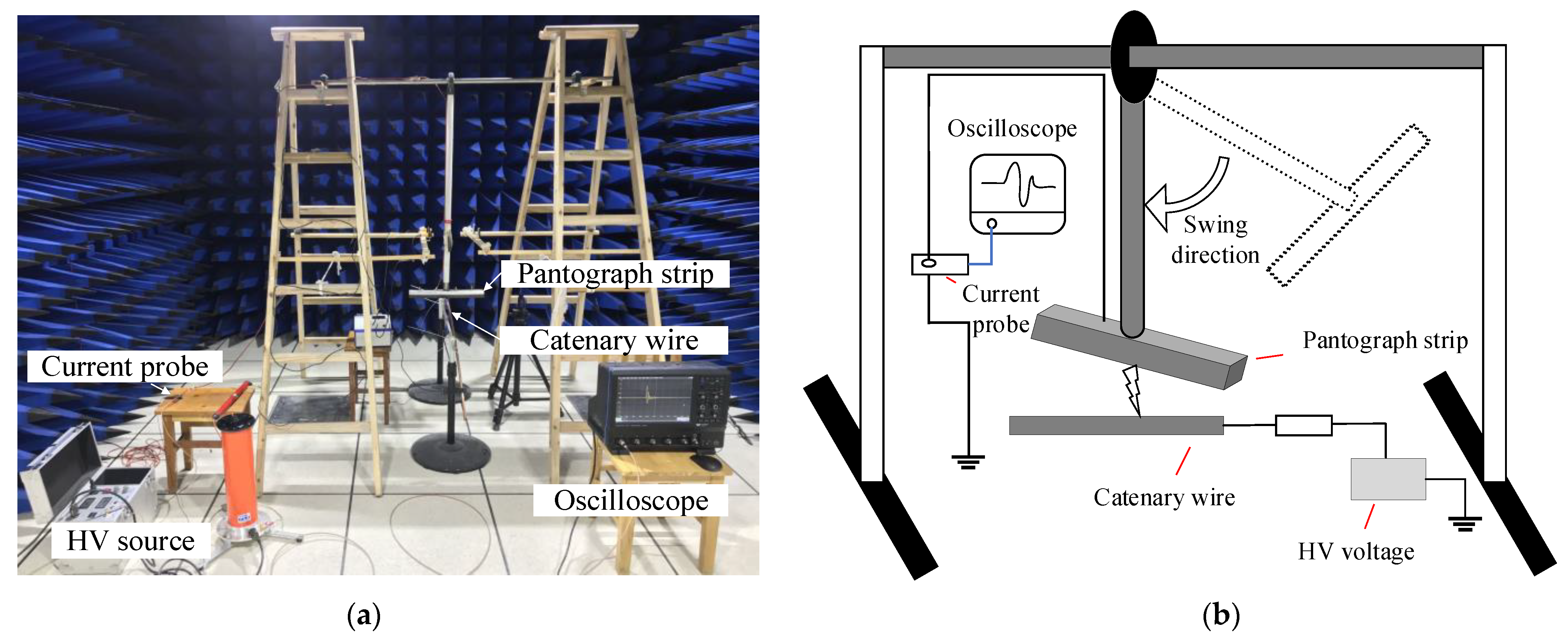
The experimental setup was built in an ultracompact anechoic chamber to examine the high-frequency behaviors generated by the arcing discharge between the pantograph strip and catenary wire (see Figure 1 and Figure 2). The two discharge electrodes are cut from the actual pantograph and catenary, respectively, which are the DSA200 and CTA120 models employed in the railway. A pendulum-typed moving electrode consists of a conducting pantograph strip affixed to the end of an insulated rod. The catenary wire is kept fixed and connected to a DC voltage source that provides a variable HV of up to 50 kV. When the contact strip swings down, the electric field between the pantograph strip and catenary wire grows with the reducing gap distance and finally exceeds the breakdown field strength, penetrating the air between the two electrodes and finally causing a conductive discharge path.

Due to the transient nature of the arc-generated electromagnetic disturbance, direct frequency-domain measurements based on frequency sweep techniques are not appropriate [28,29]. In this experiment, the time-domain waveform of the transient current from PC arcing discharge was measured using the CT-1 probe manufactured by Tektronix Company. A 1 GHz bandwidth, 20 GSa/s sampling-frequency LeCroy Waverunner 8104 digital oscilloscope was linked to the current probe via coaxial cables to acquire and record the current waveform. During the test, the oscilloscope was set as two acquisition modes: sampling rate of 10 GSa/s and acquisition time of 0.2 μs, which is enough time to record the complete current pulse of one single arc; sampling rate of 100 MSa/s and acquisition time of 10 ms when recording the repetitive series of pulses.

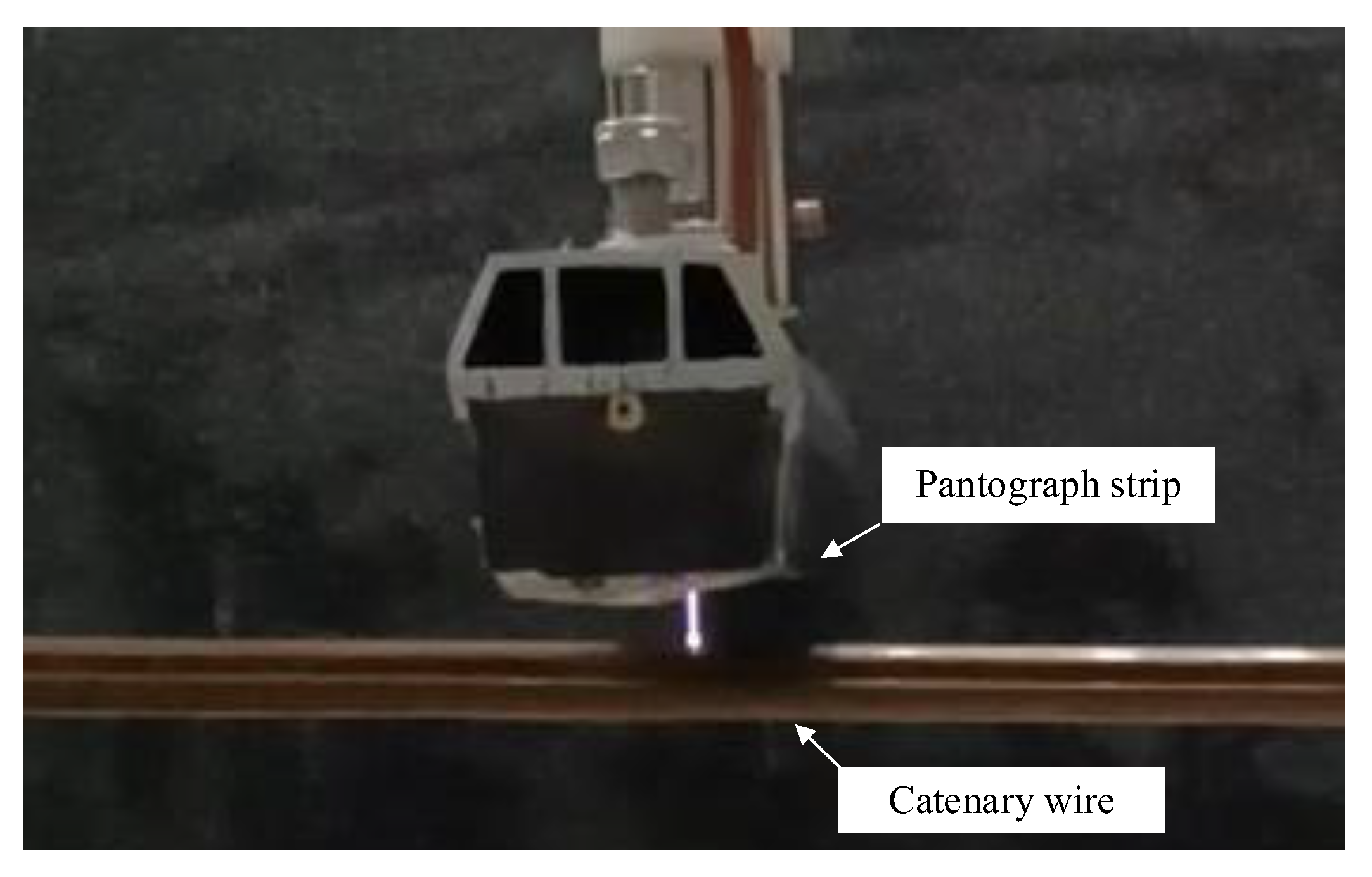
As shown in Figure 3, a typical oscilloscope recording of the time evolution of a current pulse reveals two different zones: (a) the initial high-amplitude pulse response of the transient pantograph arcing, and (b) the low-frequency decaying oscillatory tail that results in additive distortion. It should be noted that the generation of the initial pulse is due to pantograph arcing, whereas the oscillations are caused by the superposition mechanism of the reflected and incident transient currents, depending on the circuit load and the electrical parameters of the arc.

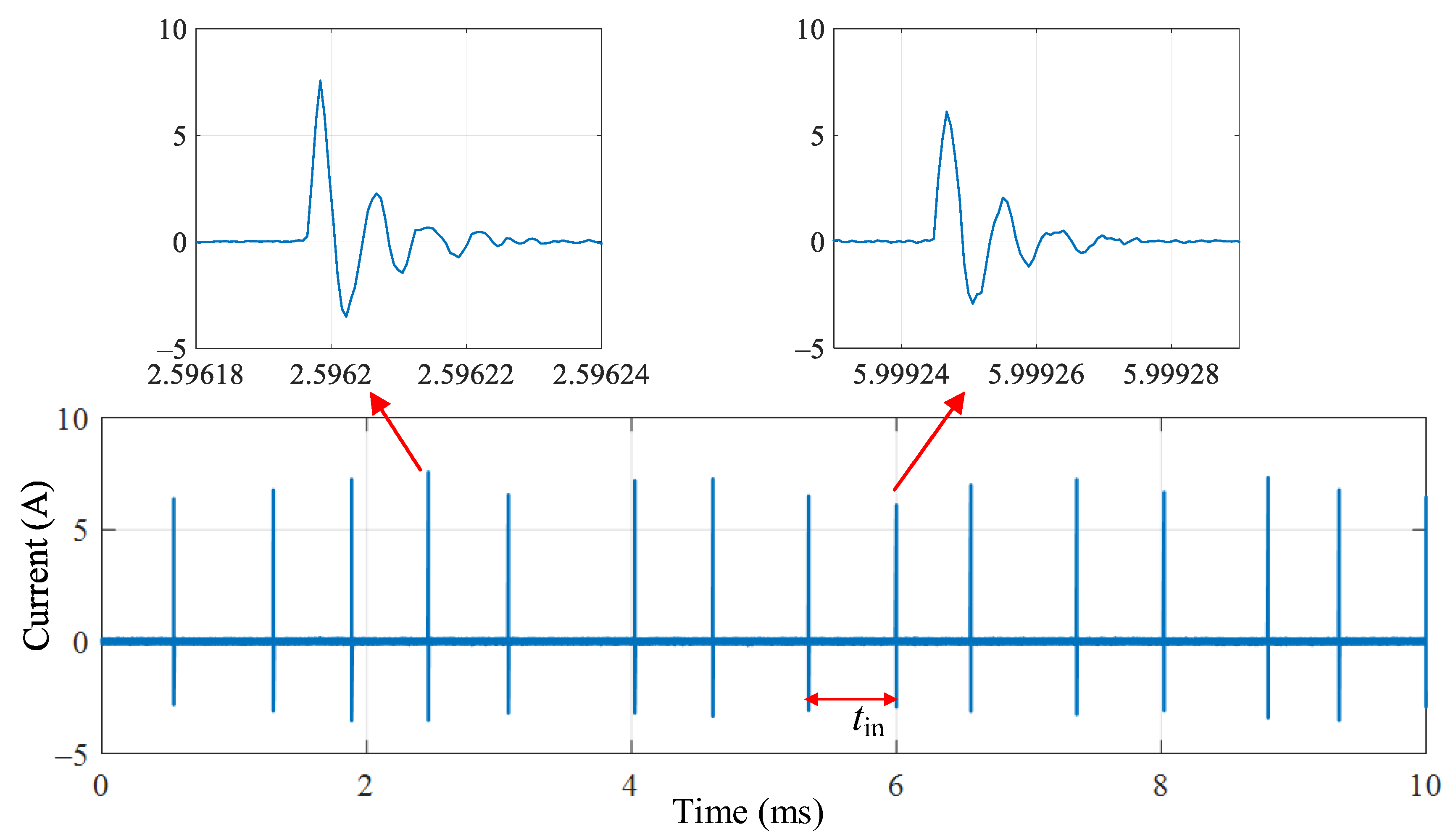
Once the arcing ignites in this experiment, the voltage drop between the electrodes will not be sufficient to keep it burning. This causes the air between the pantograph strip and the catenary wire to break down repeatedly, resulting in a series of transients of rapid arcing discharge. Consequently, when the electrode approaches, the arcing discharge current behaves as a train of pulses. Figure 4 shows the typical profile of the repeated pattern of the pulse train over a long acquisition time of 10 ms.

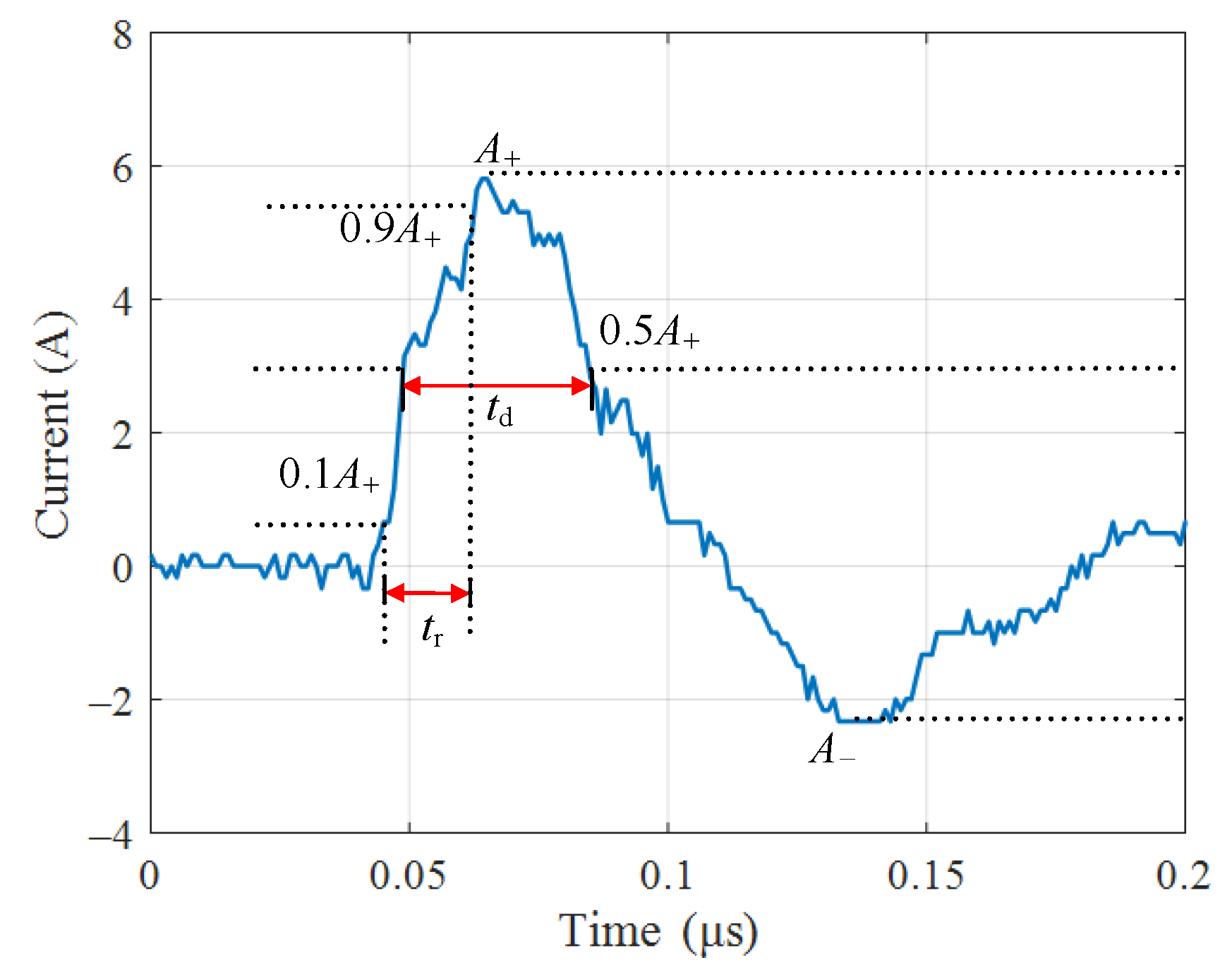
The repetitive fast transients caused by arc reignitions are measured in the time domain and evaluated in terms of peak amplitude, rise time, pulse width, successive time interval, and other specified current measures in IEC 61000-4-4 [30]. In Figure 3 and Figure 4, the time-domain waveform parameters of interest to this study are described, and they can be interpreted as follows:

• Peak amplitudes (A₊ and A₋), the positive and negative peak amplitudes of a single current pulse;
• Rise time (t_r), the time interval between the instants at which the instantaneous current value first reaches 0.1 A₊ and then 0.9 A₋;
• Pulse width (t_w), i.e., halfwave duration, the period between the instants at which the instantaneous value reaches 50% of its peak amplitude;
• Pulse repetition interval (t_in), the time interval between two successive pulses in a pulse train.

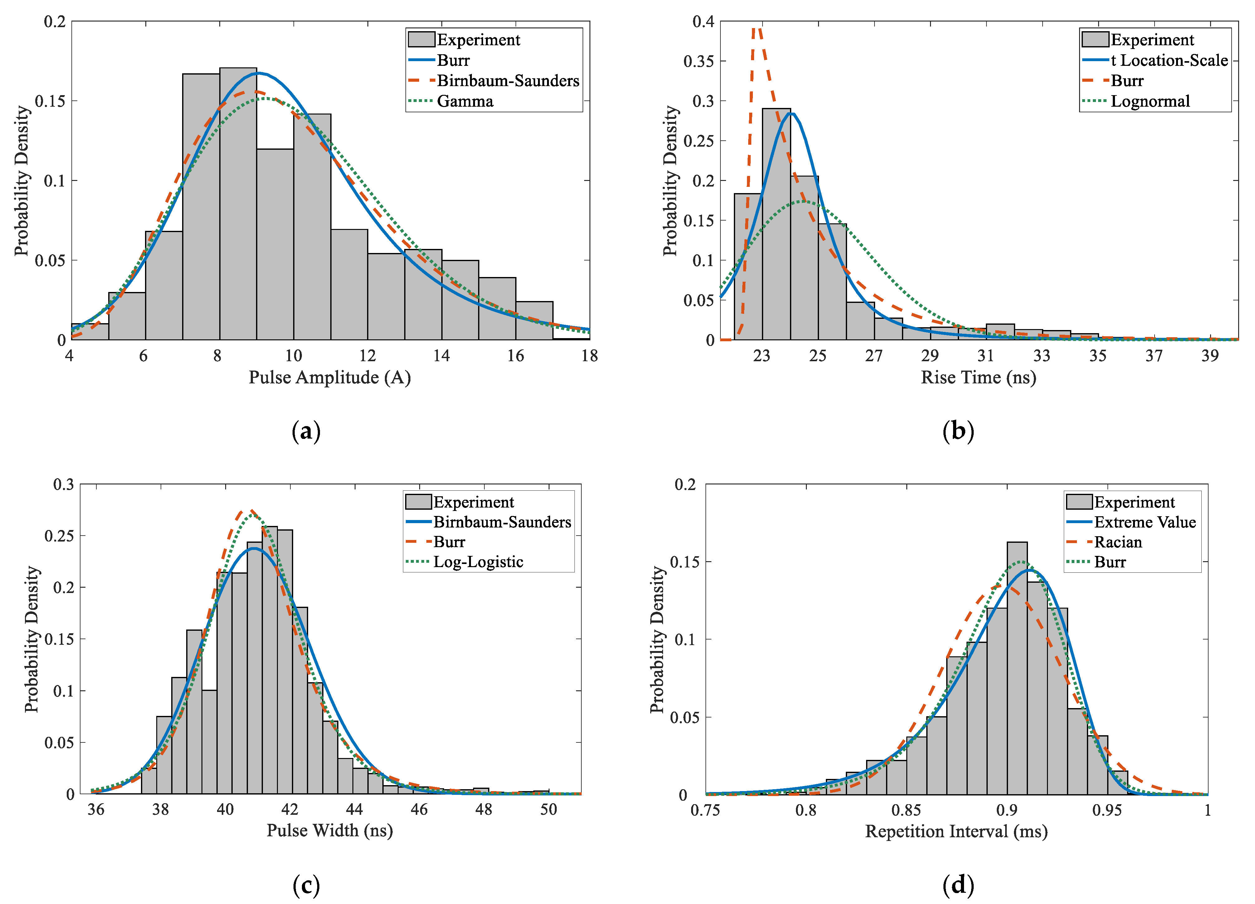
All these physical properties of the current waveform substantially affect the frequency bandwidth covered by the transient. Due to the poor reproducibility of the air discharge, a statistical investigation is required to better comprehend the characteristics of the disturbance excitation current. In Section 3, statistical evaluations of the time and amplitude characteristics of the collected transient discharge currents are presented.

3. Experimental Results and Analysis

3.1. Statistical Distribution of Transient Current Waveform Parameters

The discharge test was carried out with the sliding strip stationary, a 20 kV DC voltage, and a 5 mm discharge gap spacing as the experimental conditions. Based on the built-in Measure function of the oscilloscope, statistics of the waveform parameters were acquired. The distribution histogram of the observed peak amplitudes (A₊ and A₋), rise time (t_r), pulse width at half maximum (t_w), and interval time (t_in) of current pulses, as well as their probability density functions (PDF), are calculated with the distribution fitting tool from MATLAB software. As depicted in Figure 5, the statistical distributions of the waveform parameters with a sample size of 1000 are graphically described in the form of distribution histograms associated with various theoretical reference distributions. The characteristics of individual pulses are quite different, which is mainly reflected in the randomness of pulse amplitude, rise time, and interval time.

The optimal value of the bin width h for each histogram is determined by Scott’s rule [31], which is a formula giving a choice of the bin width for an equally spaced histogram. The rule is specified as

$$h=3.5\widehat{\sigma }{·n}^{-\frac{1}{3}},$$

(1)

where $n$ is the sample size and $\hat{\sigma }$ is the sample standard deviation.

According to Figure 5, the range of pulse amplitude distribution (taking A₊ as an example) is between 4 and 17 A, which accounts for 96.2% of the total number of samples, and the right-biased distribution of the pulse amplitude A₊ essentially follows the Burr distribution law. The rise time is predominantly distributed in the region of 23 to 27 ns, and there is less distribution in the range of 27 to 39 ns. The t Location–Scale distribution can better describe the data distribution with heavier tails (more prone to outliers). The pulse width corresponds more closely to the Birnbaum–Saunders distribution model, which results in a better fit at the distribution peak. The repetition interval time distribution of the pulse presents a left-skewed Extreme Value distribution, and the smaller the pulse interval time, the higher the repetition frequency, so the fitting accuracy on the left side of the peak is very important.

It is expected that the distribution with a close fit will result in precise predictions. Therefore, accurate distribution fitting calculations should be conducted in this section. The parameters of the selected theoretical models are estimated by the maximum likelihood (ML) method.

Table 1. Distribution fittings for the waveform parameters with different reference models.

Parameter	Reference Distribution	ML Estimation	R2	RMSE
A+	Burr	α = 9.519, c = 6.259, k = 0.983	0.894	0.018
	Birnbaum–Saunders	β = 9.593, γ = 0.277	0.873	0.020
	Gamma	a = 13.424, b = 0.742	0.856	0.021
tr	t Location–Scale	μ = 19.017, σ = 1.243, ν = 2.024	0.967	0.016
	Burr	α = 17.518, c = 228.853, k = 0.037	0.932	0.023
	Lognormal	μ = 2.981, σ = 0.117	0.743	0.044
tw	Birnbaum–Saunders	β = 40.949, γ = 0.041	0.943	0.019
	Burr	α = 40.416, c = 50.860, k = 0.696	0.942	0.021
	Log-Logistic	μ = 3.710, σ = 0.022	0.920	0.025
tin	Extreme Value	μ = 0.911, σ = 0.025	0.934	0.012
	Rician	s = 0.896, σ = 0.029	0.894	0.020
	Burr	α = 0.945, c = 40.489, k = 5.229	0.923	0.015

The bolded entries in the table are the selected reference distributions.

displays the results of parameter estimations along with two crucial goodness-of-fit indices, the coefficient of determination or R-squared (R²) and the root mean squared error (RMSE). A smaller RMSE value or an R² value closer to 1 is employed to choose a suitable model among the candidate theoretical distributions.

Although the goodness of fit tells us which reference theoretical model best describes the experimental data, it is crucial to conduct statistical hypothesis testing to see whether the ideal distribution with estimated parameters genuinely matches the empirically observed data. The Kolmogorov–Smirnov test (K–S test) is one of the frequently used hypothesis tests [32], and it is also employed in this work. The test is predicated on the most significant discrepancy between the theoretical and experimental cumulative distributions, whose statistical expression is indicated by

$$D_n= {\sup }_x \left|F_n\left(x\right)-F\left(x\right)\right|,$$

(2)

where $F_n\left(x\right)$ is the empirical cumulative distribution function (CDF) for the experiment sample and $F\left(x\right)$ is the theoretical CDF for the specified model. The operator ${\sup }_x$ denotes the supremum of the absolute differences between the empirical and theoretical CDFs. It can also be understood as the maximum vertical distance between the two cumulative probability curves, as shown in Figure 6.

The calculated K–S statistic $D_n$ is compared to the critical value $D(n,\alpha )$, related to the sample size $n$ and significance level $\alpha$, to decide whether to accept or reject the null hypothesis $H_0$: the true probability that follows the data is actually the assumed $F\left(x\right)$.

$D(n,\alpha )$ is calculated as

$$D(n,\alpha )=\frac{1.63}{\sqrt{n}},$$

(3)

when $\alpha =0.01$ and $n>50$. As the sample size for this test is 1000, the critical value for the K–S test statistic here is 0.051. The selected distribution laws and the corresponding K–S statistic results are concluded in

Table 2. K–S test for the selected distribution laws.

Parameter	Distribution Law	Dn
A+	Burr	0.047
tr	t Location–Scale	0.023
tw	Birnbaum–Saunders	0.031
tin	Extreme Value	0.034
Significance level: $\alpha =0.01$
Critical value: $D(n,\alpha )=0.051$

.

Hence, under a significance level of 0.01, the K–S test value for each parameter’s distribution estimation is smaller than the critical value for the test statistic. In light of this, it was possible to accept the $H_0$ hypothesis, which means that the actual distributions of the waveform parameters could be viewed as conforming to the distribution rule we chose.

After establishing the statistical distribution models for the waveform parameters, we compute the probability quantile points at various degrees of significance for the waveform parameters with the reference distribution models and the corresponding model parameter estimations in Table 1.

Table 3. Quantile points of the main cumulative probability of each parameter.

Cumulative Probability	Peak Amplitude (A)	Rise Time (ns)	Pulse Width (ns)	Repetition Interval (ms)
5%	5.96	15.41	38.27	0.835
50%	9.55	19.01	40.95	0.902
80%	11.94	20.33	42.39	0.923
95%	15.36	22.61	43.81	0.939

shows the calculation results with cumulative probabilities of 5, 50, 80, and 95%, representing the probability of a signal with a specific time parameter at or above a specific level, to refer to different degrees of the EMD severity. According to the theory of electromagnetic radiation, an arcing discharge generates more intense electromagnetic radiation with a steeper front-rising edge, i.e., a bigger peak amplitude or a shorter rise time, as indicated by the following equation [33]:

$$E_{\mathrm{arc}}=\frac{1}{{4\mathsf{\pi }\mathsf{\epsilon }}_0{\mathrm{c}}^2} \frac{{\mathrm{d}I}_{\mathrm{arc}}}{\mathrm{d}t}=k·\dot{I_{\mathrm{arc}}}$$

(4)

where ${\mathsf{\epsilon }}_0$ is the air’s dielectric constant, $\mathrm{c}$ is the speed of light, and $k$ is a constant. In addition, the repetition interval and pulse duration have a certain influence on the electromagnetic sensitivity of the receiving equipment, thereby affecting the effect of EMDs, which has been reported in an electromagnetic injection experiment [34].

The statistically typical current waveform parameters representing the critical EMD circumstances can be set as follows: peak amplitude of 15.36 A, rise time of 15.41 ns, pulse width of 43.81 ns, and interval time of 4.18 ms, whereas the following waveform characteristics may be selected for the excitation current characterizing the normal conditions: peak value of 9.55 A, rise time of 19.01 ns, pulse width of 40.95 ns, and interval time of 4.51 ms.

3.2. Statistical Analysis on the Peak Amplitudes of Transient Current Pulses

The procedure described in Section 3.1 for statistical hypothesis testing has demonstrated that the statistical distribution of pulse amplitudes may be characterized using the Burr distribution. The peak amplitudes of the pulsed current generated by PC discharge are influenced by the applied voltage and gap spacing between the pantograph strip and catenary line [3,4,27]. Over the whole range of relevant applied voltages and gap spacing distances, it is demonstrated that the probability densities can be approximated by the Burr distribution. This part performs a statistical analysis of the positive and negative amplitudes (A₊ and A₋) as they vary with the applied voltage and the gap spacing distance. The probability density function $f\left(A\right)$ has the following expression:

$$f\left(A\left|\alpha ,c,k\right.\right)=\frac{\frac{kc}{\alpha }\cdot {\left(\frac{A}{\alpha }\right)}^{c-1}}{{\left(1+{\left(\frac{A}{\alpha }\right)}^c\right)}^{k+1}},$$

(5)

where $A$ is the pulse amplitude, and $\alpha ,c,k$ are the shape parameters for the distribution.

Figure 7 shows the measured distribution and fitting probability densities of PC discharge current amplitudes for different applied voltages U and gap spacing distances d. Under experimental conditions in which the applied voltage varied from 20 kV to 35 kV and the gap spacing distance changed from 5 mm to 15 mm, the waveform parameters defined above were all picked up in the experiment.

As depicted in Figure 7a–d, under the same contact spacing length, the peak amplitudes of the pulsed current (both A₊ and A₋) increase with higher applied voltages, primarily due to the occurrence of multi-point discharges caused by the strengthening electric field. Positive and negative peak amplitudes increase significantly more in the lower voltage range of 20 to 25 kV, whereas the distribution of peak amplitudes varies little and stabilizes gradually in the higher voltage range of 25 to 35 kV. Figure 7d–f shows that, despite a constant applied voltage, the peak value of the current pulse increases considerably as the distance of the contact gap increases. The influence of the gap spacing on the peak amplitudes of the discharge current can be explained as follows: a greater d allows a space charge to travel a greater distance, resulting in the accumulation of more charges and a reduction in the total electric field. The decrease of the total electric field weakens the discharge at the conductor’s surface, hence reducing the number of seed charges at the beginning of the discharge and the peak amplitudes of the resulting discharge pulse.

Under identical applied voltage and gap spacing conditions, the positive amplitude distribution is to the left of the negative amplitude distribution, suggesting that most positive peak values are greater than the negative ones. At the same time, the distribution shape of A₋ is more compact than that of A₊, indicating that the variance of A₋ is significantly smaller. Comparing the average values of A₊ and A₋ with various applied voltages reveals that the changes of A₊ with the applied voltages are comparable to those of A₋, and that the average values of the two are nearly twice as close. Figure 8 depicts scatter plots for A₊ versus A₋ under different settings, showing the value relationship between A₊ and A₋ from a single current pulse. From the plots, we can observe a generally tight positive correlation between the positive peak amplitudes of the pulsed current and its negative peak amplitudes, which indicates a nearly identical ratio between A₊ and A₋ under the same condition. The ratio of the positive peak amplitude A₊ and the following negative peak amplitude A₋ in one single current pulse can be expressed as

$$R_{\mathrm{A}}=\frac{A_{+}}{A_{-}},$$

(6)

and it is believed to be related to the arc generation conditions, as depicted in Figure 8.

In order to explore the impact of the applied voltage and electrodes’ gap spacing distance on R_A, the variation of R_A at different voltages from 20 to 40 kV with gap spacing distance changes from 5 to 15 mm is shown in Figure 9. The average values and standard deviations (STD) are used to represent the fluctuations of R_A in this figure.

According to Figure 9, R_A increases with d; however, at the same spacing, R_A maintains a constant value while U changes from 20 kV to 40 kV, showing that the applied voltage has no influence over R_A. This phenomenon is thought to be brought on by a variation in the arc length, or the distance between the electrodes, which changes the arc resistance. The arc resistance R_arc can be expressed using the following formula with reference to [33] when the arc is thought of as a plasma cylinder.

$$R_{\mathrm{arc}}=\frac{\rho l}{S},$$

(7)

where l represents the spacing distance and S represents the average cross-sectional area of the arc column. The resistivity of the arc in the expression is written as ρ with the unit of Ω m, which is thought to be related to gas properties and the number of ionized particles in arc plasma between the contacts. From Equation (7), we can see that the arc resistance increases when the contact separation distance increases. Given that the formation of a series RLC path by the discharge accounts for the current waveform of the oscillation decay mode in Figure 3, the following expression describes the relation between the oscillation’s damping ratio factor and the arc’s electrical parameters:

$$\zeta =\frac{R_{\mathrm{arc}}}{2} \sqrt{ \frac{C}{L} }.$$

(8)

Consequently, a larger arc resistance increases the damping coefficient, which reduces the oscillation effect of the discharge circuit and leads the RLC circuit to transition from an underdamped to an overdamped state. As illustrated in Figure 9, the ratio of the positive peak amplitude to the subsequent negative peak amplitude in a single current pulse increases as the electrodes’ gap spacing distance increases.

3.3. Statistical Analysis on the Pulse Repetition Intervals

The repeated pattern of the discharge current pulse generated by PC arcing is shown in Figure 4. The pulse repetition frequency $f_{\mathrm{R}}$ can be described using the following equation, with the applied voltage as a variable, similar to the narrow-gap Trichel pulse.

$$f_{\mathrm{R}}{=K}_{\mathrm{R}}(U-U_0{)}^2,$$

(9)

where $K_{\mathrm{R}}$ is the ratio constant and U₀ is the coefficient that adjusts the applied voltage value to match the experimental data more closely. The physical significance of U₀ is the inception voltage of the arcing discharge. However, Equation (9) is insufficient to describe the changing law of the repetition frequency with varying gap spacing distances. Fortunately, close correlations between K_R and d as well as U₀ and d were found in the experiments, as shown in Figure 10. The fitted relational expression between K_R and d exhibits a power law:

$$K_{\mathrm{R}}=0.018{·d}^{-0.513},$$

(10)

whereas U₀ and d exhibit a linear association because of the linear relationship between the breakdown field strength and the gap distance,

$$U_0=0.788·d+4.136,$$

(11)

where the units for K_R, U₀, and d are expressed in kHz, kV, and mm, respectively.

Due to the inversely proportional relationship between the average value of the repetition intervals and the pulse repetition frequency, the average value of the time intervals between two subsequent pulses in a pulse train has the following expression:

$$\overline{t_{\mathrm{i}}}{=K}_{\mathrm{i}}\frac{1}{{\left(U-U_0\right)}^2} ,$$

(12)

where

$$K_{\mathrm{i}}=\frac{1}{K_{\mathrm{R}}} .$$

(13)

By substituting Equations (10), (11) and (13) into Equation (12), the fitted equation for the mean value of the repetition intervals can be given as

$$\overline{t_{\mathrm{in}}}=\frac{1}{0.018{·d}^{-0.513}} · \frac{1}{{\left(U-0.788·d-4.136\right)}^2}.$$

(14)

The interval time $t_{\mathrm{in}}$ follows the Extreme Value distribution mentioned above, which has a leftward skewed form that is constant for all parameter values. The location parameter, $\mu$, shifts the distribution along the real line, and the scale parameter, $\sigma$, expands or contracts the distribution. The Extreme Value distribution is expressed in PDF form as follows:

$$f\left(t_{\mathrm{in}}\left|\mu ,\sigma \right.\right)={\sigma }^{-1}\exp (\frac{t_{\mathrm{in}}-\mu }{\sigma })\exp (-\exp (\frac{t_{\mathrm{in}}-\mu }{\sigma })).$$

(15)

After obtaining the mean value $\overline{t_{\mathrm{in}}}$ and the standard deviation $s_{\mathrm{in}}$ of the sample, we can use the equation in Ref. [35] to determine the estimated values of $\mu$ and scale parameter $\sigma$:

$$\left\{\begin{array}{c}\mu =\overline{t_{\mathrm{in}}}+0.577\sigma \\ \sigma =\frac{s_{\mathrm{in}}}{1.283}\end{array}\right.$$

(16)

A correlation between the mean and standard deviation of the measured $t_{\mathrm{in}}$ is displayed in

Table 4. Correlation between the mean and standard deviation of the measured t_in.

Experimental Condition	Mean Value (ms)	Standard Deviation (ms)	CV (%)
U = 20 kV, d = 5 mm	0.905	0.310	34.3
U = 25 kV, d = 5 mm	0.453	0.157	34.7
U = 30 kV, d = 5 mm	0.243	0.083	34.1
U = 35 kV, d = 5 mm	0.185	0.064	34.8
U = 35 kV, d = 10 mm	0.312	0.109	35.1
U = 35 kV, d = 15 mm	0.571	0.196	34.4

. The mean and standard deviation of $t_{\mathrm{in}}$ are positively correlated across samples under different experimental settings, as observed. In this instance, the coefficient of variation (CV), defined as the ratio of standard deviation to mean, is used to indicate the accuracy of a measurement. The calculated CVs under various voltage and gap spacing conditions are listed in Table 4, and it appears that the CV value in this experiment remains constant. Therefore, after knowing the applied voltage and gap spacing distance, it is possible to estimate the mean value and standard deviation of the repetition intervals, compute the estimated $\mu$ and $\sigma$, and derive the PDF expression of $t_{\mathrm{in}}$ for this particular condition.

3.4. Statistical Study of Transient Current Pulse Rise Time and Pulse Width

The statistical distribution of the current rise time t_r follows the t Location–Scale model, represented as

$$f\left(t_{\mathrm{r}}\left|\mu ,\sigma ,\nu \right.\right)=\frac{\mathsf{\Gamma }(\frac{\nu +1}{2})}{\sigma \sqrt{\nu \pi }\mathsf{\Gamma }(\frac{\nu }{2})}{[\frac{\nu +(\frac{t_{\mathrm{r}}-\mu }{\sigma }{)}^2}{\nu }]}^{-(\frac{\nu +1}{2})},$$

(17)

where Γ(•) is the gamma function, $\sigma$ is the scale parameter, $\mu$ is the location parameter, and $\nu$ is the shape parameter. The distribution parameters that characterize the statistical distribution of t_r under various experimental settings are determined using the ML estimation approach with a 95% confidence interval.

Table 5. Fitted distribution parameter of t_r.

Experimental Condition	$\mathbf{Location}\mathbf{Parameter}\mathbf{\mu }$	$\mathbf{Scale}\mathbf{Parameter}\mathbf{\sigma }$	$\mathbf{Shape}\mathbf{Parameter}\mathbf{\nu }$
U = 20 kV, d = 5 mm	19.017	1.243	2.024
U = 25 kV, d = 5 mm	18.681	1.229	2.019
U = 30 kV, d = 5 mm	19.118	1.235	2.014
U = 35 kV, d = 5 mm	18.731	1.143	2.023
U = 35 kV, d = 10 mm	20.032	1.361	2.026
U = 35 kV, d = 15 mm	20.889	1.585	2.024

demonstrates that the applied voltage has no direct relationship with the distribution parameter values; however, examining the data for different gap spacing distances reveals an evident correlation between the gap spacing distance d and the location parameter $\mu$, as well as the scale parameter $\sigma$. During the condition shifting, the shape parameter $\nu$ maintains a constant value near 2.02. The fitting relation between $\mu$ and d can be described as

$$\mu =0.216d+17.732.$$

(18)

Additionally, the fitting relation between $\sigma$ and d is as follows:

$$\sigma =0.044d+0.921.$$

(19)

The Birnbaum–Saunders distribution model, whose PDF has the following form, is used to describe the statistical distribution of the pulse width t_w.

$$f\left(t_{\mathrm{w}}\left|\beta ,\gamma \right.\right)=\frac{1}{\sqrt{2\pi }}\exp \{-\frac{\sqrt{t_{\mathrm{w}}/\beta }-{\sqrt{\beta /t_{\mathrm{w}}}}^2}{2{\gamma }^2}\}\frac{\sqrt{t_{\mathrm{w}}/\beta }+{\sqrt{\beta /t_{\mathrm{w}}}}^{}}{2\gamma t_{\mathrm{w}}},$$

(20)

where β is the scale parameter and γ is the shape parameter. According to the calculated parameters by the ML approach in

Table 6. Fitted distribution parameter of t_w.

Experimental Condition	Scale Parameter β	Shape Parameter γ
U = 20 kV, d = 5 mm	40. 949	0.041
U = 25 kV, d = 5 mm	39.681	0.038
U = 30 kV, d = 5 mm	39.562	0.041
U = 35 kV, d = 5 mm	38.169	0.039
U = 35 kV, d = 10 mm	37.124	0.038
U = 35 kV, d = 15 mm	38.758	0.039

, neither the varying applied voltage nor the changing gap spacing distance has a close relationship with the distribution parameter values for the Birnbaum–Saunders model. This result shows that although the pulse width of a single discharge pulse follows a given distribution rule under different conditions, the distribution law does not change with the arc generation conditions.

4. Deviation of the Stochastic Model of Arcing Currents

The fundamental concept underlying the stochastic model of the pantograph–catenary arcing discharge pulse is to construct current pulse sequences with similar statistical properties and similar shapes to the measurement results. Single pulses and continuous pulse trains are both considered in constructing the time domain waveform of the arcing current. The single pulse waveform model is constructed using the main waveform parameters obtained from the above statistical analysis to construct the single pulse waveform function, while the continuous pulse model generates a continuous long pulse sequence with statistical properties similar to the measurement results by splicing together multiple single pulses based on the obtained single pulse waveform.

Considering the bipolar characteristic of a measured single current pulse, we suggest that a typical waveform comprised of two modified double exponential functions be used to fit the single pulse, which is expressed as follows:

$$I\left(t\right)=\left\{\begin{array}{cc}{A}_{+} k_1{(\mathrm{e}}^{-{\alpha }^2{t}^2}-{\mathrm{e}}^{-{\beta }^2{t}^2}),\hfill & {0<t<t}_{\mathrm{p}}\hfill \\ -A_{-} k_2{(\mathrm{e}}^{-{\alpha }^2{(t-t_{\mathrm{p}})}^2}-{\mathrm{e}}^{-{\beta }^2{(t-t_{\mathrm{p}})}^2}),\hfill & t_{\mathrm{p}}{<t<t}_{\mathrm{e}}\hfill \end{array}\right.$$

(21)

where $k_1$ and $k_2$ are the constants determined by a fitting procedure for the measured waveform, $\alpha$ and $\beta$ are the mathematical parameters awaiting translation from the physical parameters, t_p is the zero-crossing point of the positive pulse component, and t_e is the end time of the single current pulse.

The modified double exponential function (MDEF) employed in Equation (21) was introduced in Ref. [36] and is derived from the popular double exponential pulse (DEP) function that is given by

$${I\left(t\right)=I}_0{k(\mathrm{e}}^{-\alpha t}-{\mathrm{e}}^{-\beta t}),$$

(22)

where $I_0$ is the function’s maximum, $k$ is a modifying factor, and α and β are characteristic parameters. The DEP function was presented to characterize the shape features of electromagnetic pulse waveforms with t_r of several nanoseconds and t_w of tens of nanoseconds, whereas the MDEF model was proposed to characterize pulses with low t_w/t_r ratios.

Given that the rise edges of pulses acquired in some experiments are noticeably less steep than the standard DEP and their fall edges are obviously steeper, it is natural to find a modified method that squares the index in the DEP function to characterize the waveform shape by stretching the rise edge and compressing the fall edge. The MDEF is written as follows:

$${I\left(t\right)=I}_0{k(\mathrm{e}}^{-{\alpha }^2{t}^2}-{\mathrm{e}}^{-{\beta }^2{t}^2}).$$

(23)

In practice, the physical characteristics of a pulse, typically the rise time t_r, pulse width at half maximum t_w, and fall time t_f (the time interval from 90% to 10% of the maximum value), and the function’s mathematical parameters, denoted as α and β, commonly need to be transformed into each other with high precision. Using the numerical solution and asymptotic formulations to make estimations, Ref. [36] established the correlations for βt_w, t_w/t_r, and t_f/t_r with β/α for Equation (23), which are expressed as follows:

$${\beta t}_{\mathrm{w}}\approx 5.088\exp \left(\right(\frac{\beta }{\alpha })/9.871)-4.474,$$

(24)

$$\frac{t_{\mathrm{w}}}{t_{\mathrm{r}}}\approx 0.191\exp \left(\right(\frac{\beta }{\alpha })/1.732)+1.615,$$

(25)

$$\frac{t_{\mathrm{f}}}{t_{\mathrm{r}}}\approx 0.0057\exp \left(\right(\frac{\beta }{\alpha })/0.387)+1.584.$$

(26)

Suppose the probability distributions of the waveform parameters are known. In that case, four arrays of random numbers, which describe the positive amplitude (A₊), rise time (t_r), pulse width (t_w), and separation intervals (t_in) of current pulses, can be obtained through a pseudo-random number generation algorithm. The proportion ratio between the positive and negative amplitudes at different voltages, shown in Figure 9, can be used to calculate the negative amplitude (A₋). The mathematical parameters α and β are calculated with Equations (24) and (25), which, in turn, can be used to estimate the fall time t_f in Equation (26) to determine t_p and t_e in the following equation.

$$\left\{\begin{array}{c}{t}_{\mathrm{p}}\approx 1.35{(t}_{\mathrm{r}}{+t}_{\mathrm{f}})\\ t_{\mathrm{e}}\approx 2.70{(t}_{\mathrm{r}}{+t}_{\mathrm{f}})\end{array}\right..$$

(27)

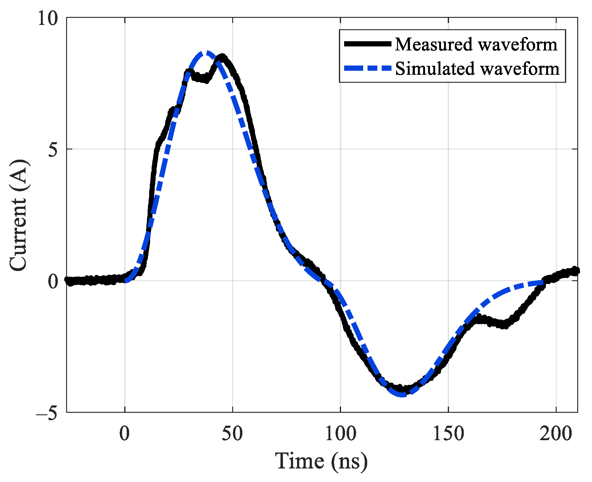
By substituting these mathematical parameters into Equation (21), the analytical equation representing the time domain variation of a single pulse can be determined. Figure 11 illustrates the measured waveform and simulated sequence of a single arcing current pulse when the applied voltage is 20 kV and the gap spacing distance between electrodes is 5 mm. The observed waveform is depicted as a solid black line, whereas the simulated waveform is shown as a dashed blue line. In addition, the function parameters and physical properties of the discharge current are listed beneath the figure. The measured and calculated waveforms have a correlation coefficient of roughly 0.956, which confirms the validity of the proposed generation method for a single pulse.

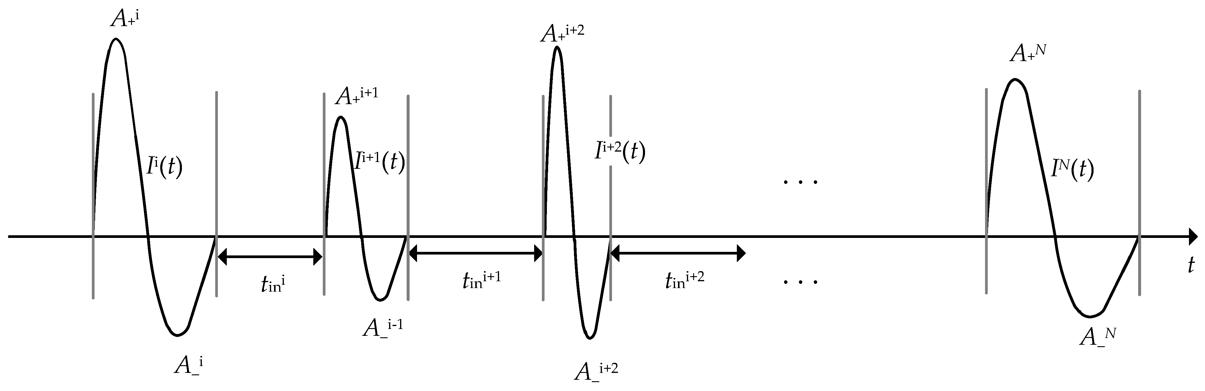
Regarding the current pulse trains, they can be characterized as the superposition of separated single current pulses. A schematic representation of a typical arcing current pulse train with pseudo-randomly generated parameters is shown in Figure 12. $A_{+}^{\mathrm{i}}$ and $A_{-}^{\mathrm{i}}$ are the positive and negative amplitudes for the ith current pulse, respectively, and $t_{\mathrm{in}}^{\mathrm{i}}$ is the ith interval time between two successive pulses. According to the above analysis, the analytical function of every single pulse can be determined according to the triplet (A+, t_r, t_w) generated by the parameter distribution functions. Assuming N to be the total number of single pulses in a pulse train, the N single pulses can be represented by the notation $I^{\mathrm{i}}\left(t\right)$, $1<\mathrm{i}<N$. Then, we can produce N groups of random t_in based on the Extreme Value distribution stated in Equation (15) and apply the following formula to splice the pulse train sequence:

$$I_{\mathrm{train}}\left(t\right)={\displaystyle \sum }_{\mathrm{i}}{I}^{\mathrm{i}}\left(t\right)+{\displaystyle \sum }_{\mathrm{i}}{S}^{\mathrm{i}}\left(t\right), 1<\mathrm{i}<N$$

(28)

where $S^{\mathrm{i}}\left(t\right)$ denotes the current value between the end of ith pulse (denoted as $t_{\mathrm{ei}}$) and the start point of the (i + 1)th pulse (denoted as $t_{\mathrm{s}(\mathrm{i}+1)}$). $S^{\mathrm{i}}\left(t\right)$ has following expression:

$$S^{\mathrm{i}}\left(t\right)=0,t_{\mathrm{ei}}<t<t_{\mathrm{s}(\mathrm{i}+1)},$$

(29)

and $t_{s(i+1)}-t_{\mathrm{ei}}$ is the random pulse interval time $t_{\mathrm{in}}^{\mathrm{i}}$.

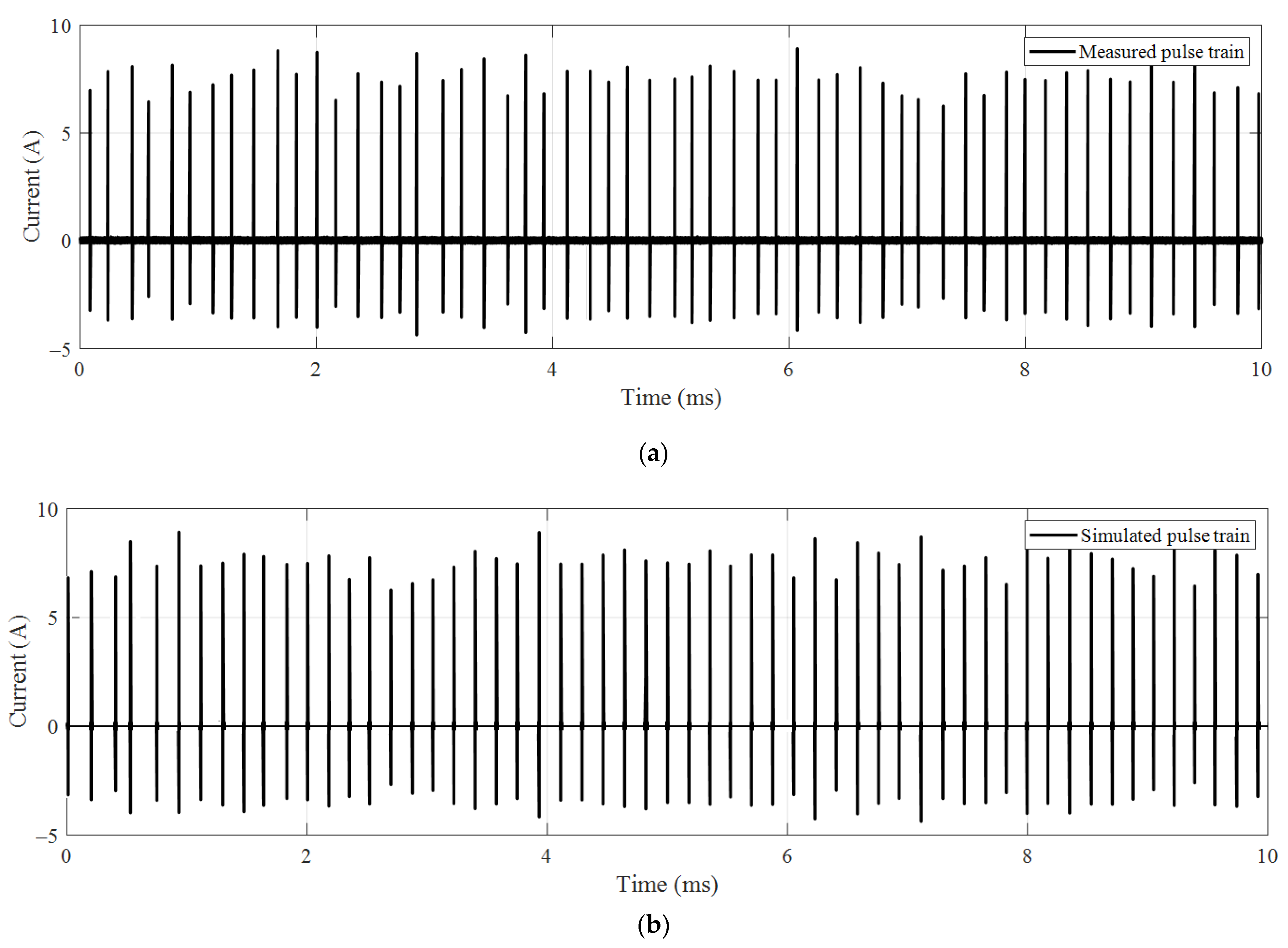
As an example, the measured and fitted waveforms of the discharge pulse train recorded for 10 ms are presented in Figure 13a,b, respectively, where the applied voltage is 35 kV and the gap spacing between electrodes is 5 mm. It is seen that both the amplitude of each pulse in the test waveform and the simulated sequence, as well as the interval between two consecutive pulses, are random and that their randomness is similar. By statistical calculation, $\overline{t_{\mathrm{in}}}=0.185$ ms and $s_{\mathrm{in}}=0.064$ ms. Then, we calculated the parameter value of the Extreme Value distribution from Equation (16), and we have $\mu$ = 0.214 and $\sigma$ = 0.050. The interval distance of the simulated pulse train in Figure 13b is produced at random according to Equation (15). With this determined PDF, the generated t_in has a mean value of 0.185 and a standard deviation of 0.064, consistent with statistical calculations. The pulse train simulated by this method is very similar to the measured one. The stochastic model of the discharge waveform is effective based on the description of the statistical distribution of the waveform.

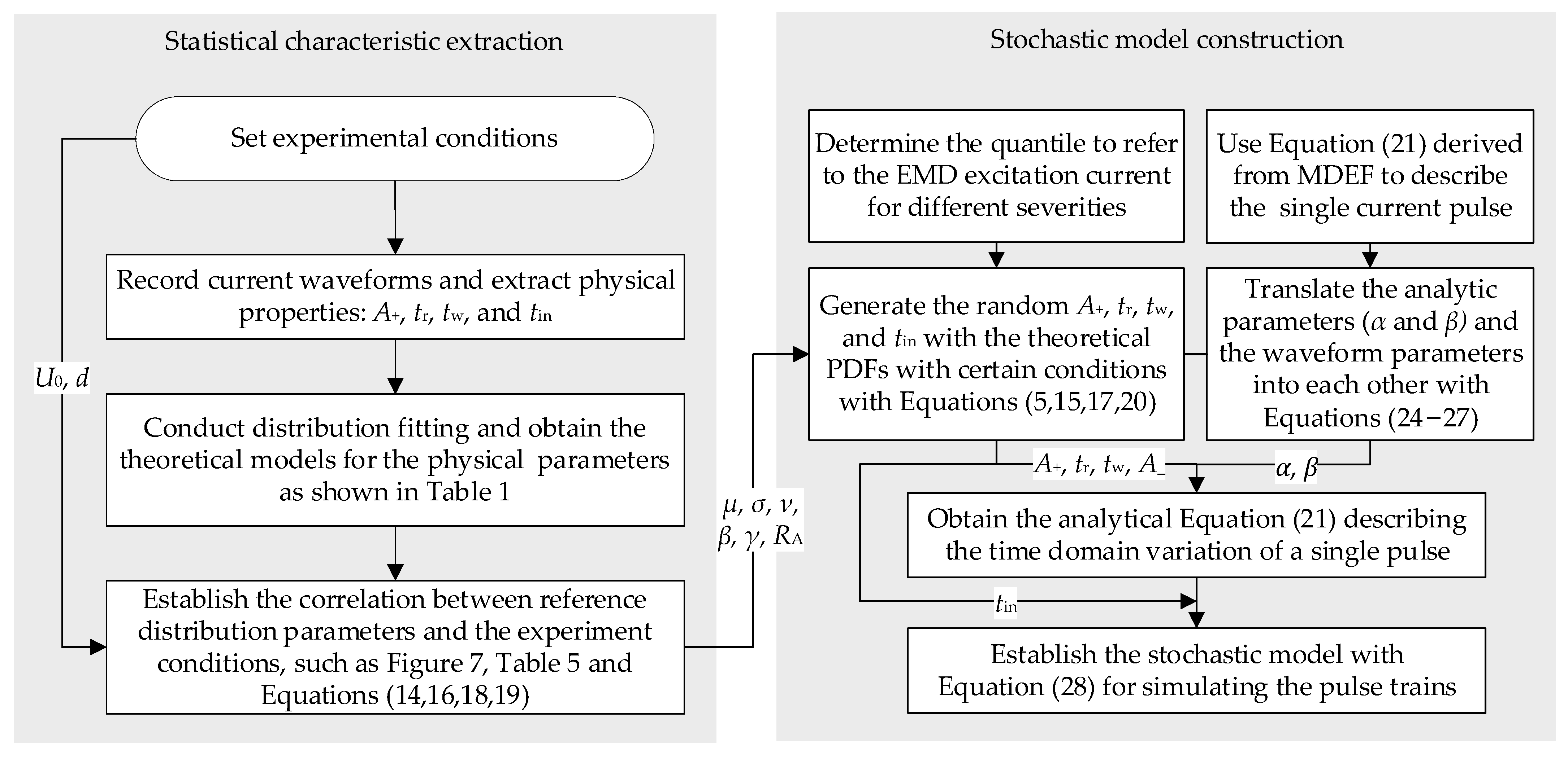
The flow diagram of the stochastic model of pulsed discharge current in the time domain is summarized in Figure 14, including the extraction for the statistical distribution of the waveform parameters, the construction of connection between the mathematical parameters (α, β, t_p, t_e) and physical parameters (A₊, A₋, t_r, t_w, t_in, t_f), and the establishment of the time-domain waveform of the transient current for both single pulse and pulse train. The detailed description of the calculation process has been given in previous sections.

According to the method depicted in the flowchart, the excitation current waveforms of EMD with various intensities can be obtained in the case of a known parameter distribution function by altering the quantile of the selected probability distribution.

We first chose the 50%, 80% (or 20%), and 95% (or 5%) quantiles to represent the moderate, severe, and critical EMD scenarios. Each waveform characteristic conforms to a specific distribution rule, although the distribution parameters still need to be specified. In fact, the parameters of each distribution function can be determined by the experimental conditions according to the correlation shown in Figure 7, Table 5, and Equations (14), (16), (18) and (19). Then, A₊, t_r, t_w, and t_in with statistically typical characteristics can be obtained from the identified distribution function and the selected quantiles for different severity levels. Using the relationship between the analytic parameters (α and β) and the waveform parameters in Equations (24)–(27), the MDEF model (in the form of Equation (21)) representing the single pulse waveform can be finally derived from the triplet (A₊, t_r, t_w).

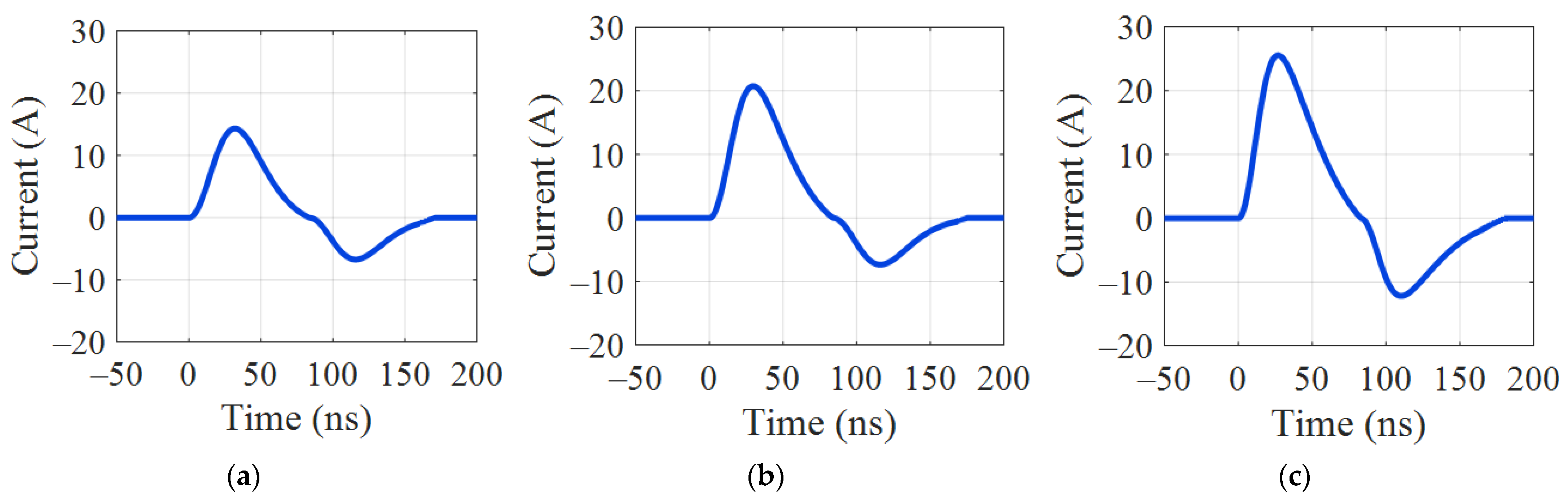
The approach can generate the arc discharge current waveform for a specified EMD severity and arc-generating condition. Figure 15 illustrates the calculated single-pulse current waveforms for the three situations with an applied voltage of 35 kV and an electrode separation spacing of 5 mm.

Comparing the three generated waveforms, the positive peak amplitudes are 14.580, 19.218, and 26.252 A, respectively, while the rise times are 18.731, 17.522, and 15.419 ns, which proves a larger amplitude and a faster rising speed dI/dt in the more serious situations. In addition, the calculated quantiles of the pulse interval times representing the three situations are 0.195, 0.139, and 0.065 ms. In a more serious EMD scenario, not only does a single current pulse exhibit a higher and steeper front-rising edge, but the occurrence frequency of the pulsed current transients increases significantly.

The method first establishes the connection between the arc generation conditions and the probability distribution of physical waveform characteristics. Then, it uses the relationship between these waveform parameters and the function parameters to determine the analytical expression that can estimate the current waveform. The proposed method can provide electromagnetic excitation current waveforms under different EMD severities and arcing conditions with high accuracy across the entire variation range of the experimental parameters. It can even generate the estimated waveform of arcing current beyond the experimental parameters’ variation range if the empirical fitting results conform to the physical law, which can be used as prediction of the current waveforms and their key parameters.

The application of this method can further elucidate the generation mechanism of the electromagnetic emission from PC arcing and supplement the fundamental data of EMD created by pantograph–catenary arcing. The generated pulse waveform can be utilized in assessing the immunity of the device under test to the EMD generated by pantograph–catenary arcing. As the electromagnetic excitation source, the generated waveform can help reproduce the electromagnetic environment when a pantograph–catenary arc occurs.

5. Conclusions

This research investigates the time characteristics of the EMC excitation current produced by PC arcing discharge based on a large sample of waveform data recorded from laboratory experiments. The analysis of this data leads to the following conclusions:

• The statistical distribution of pulse peak amplitude, rise time, pulse width at half maximum, and pulse interval time follows a specific reference distribution determined by the distribution fitting method. The chosen reference distribution model was validated through a Kolmogorov–Smirnov hypothesis test.
• Statistical analysis demonstrates that the distribution parameters of each fitted model vary with the applied voltage and the gap spacing distance between the electrodes. The fitting relation between the waveform parameters and the experimental conditions is established using a maximum likelihood estimation approach. This allows for the determination of statistically typical current waveform parameters representing different EMD severities and parameters in the later deduced current function.
• A new bipolar MDEF is introduced to describe the amplitude of the PC arcing current as a function of time, and is used to model the ratio between the positive and negative peak amplitudes, which increases with a larger gap spacing. The mathematical parameters of the bipolar MDEF are calculated from the waveform parameters generated by a pseudo-random number generation algorithm, based on the known time characteristics’ statistical distributions. The measured and calculated waveforms show a correlation coefficient of approximately 0.956, confirming the validity of the proposed generation method for a single pulse.
• The PC discharge current pulse train is characterized as the superposition of separated single current pulses generated by the stochastic model. The simulated pulse train closely matches the measured one, indicating that the stochastic model of the discharge waveform is effective in describing the statistical distribution of the waveform.

Overall, this study provides valuable insights into the time characteristics of the EMD excitation current produced by PC arcing discharge, and offers a new method for generating PC arcing current waveforms with a high degree of accuracy. The subsequent research focused on reconstructing the electromagnetic environment that occurs during PC arcing. The research team will achieve this by developing a miniaturized electromagnetic environment simulator for pantograph–catenary discharge using the calculated statistically typical EMD excitation current and PC radiation structure. This simulator can replicate the conditions of PC arcing electromagnetic emissions, aiding in a better understanding of this phenomenon.