DV-Hop Location Algorithm Based on RSSI Correction

Abstract

To increase the positioning accuracy of Distance Vector-Hop (DV-Hop) algorithm in non-uniform networks, an improved DV-Hop algorithm based on RSSI correction is proposed. The new algorithm first quantizes hops between two nodes by the ratio of the RSSI value between two nodes and the benchmark RSSI value, divides the hops continuously, calculates the average hop distance according to the Minimum Mean Square Error (MMSE) criterion of the best index based on the quantized hops, and then adds hop distance matching factor to the fitness function of each anchor node into the calculation of the hop distance fitness function to weight the fitness function. The change index value is introduced to obtain more accurate hop distance value, and then the estimation error of unknown node (UN) coordinate is modified by using the distance relationship between the UN and the nearest beacon node (BN), and the modified coordination position is further modified by using the triangle centroid to improve the accuracy of node positioning in the irregular network. The experimental results show that compared with the original DV-Hop, improved DV-Hop1, improved DV-Hop2 and improved DV-Hop3, the localization error of the improved algorithm in this paper is reduced by 58%, 45%, 34%, and 29%, respectively, on average, in the two network environments. Without increasing the hardware cost and energy consumption, the improved algorithm has excellent localization performance.

1. Introduction

Wireless Sensor Networks (WSNs) enable IoT to obtain the required monitoring information. Node location is the key to WSNs monitoring information collection. Without location information, monitoring information will lose its meaning [1,2,3]. Therefore, node location has become an issue in WSNs and a research hotspot [4]. The precision of node location determines if the monitoring information can be related to the perceived phenomenon source, so it is crucial to ensure that nodes can obtain accurate location information [5]. However, in large WSNs, it is unrealistic to equip each sensor node with a GPS (Global Positioning System) chip to obtain position information [6]. A more reasonable solution is to allow some sensor nodes to obtain their own positions by equipping them with GPS, which are called beacon nodes (BNs), and estimate the locations of other nodes (nodes with unknown positions) by communicating with BNs.

On the basis of whether to measure the distance or azimuth between two nodes or not, there are two kinds of positioning algorithms—location algorithm based on distance measurement and location algorithm without distance measurement [7]. The ranging technology required by the range-based positioning algorithm mainly includes Receive Signal Strength Indicator (RSSI), Time of Arrival (TOA), Time Difference of Arrival (TDOA) Angle of Arrival (AOA), etc. [8]. Location algorithms without ranging mainly include centroid algorithm, convex programming algorithm, DV-Hop algorithm, etc. [9].

Among location algorithms without range measurement, more and more researchers are paying attention to DV-Hop because of its simplicity and scalability [10]. In order to further improve the location accuracy of DV-Hop algorithm, researchers have tried many improvement strategies. Fei Tang [11] proposed a new DV-Hop location algorithm based on Simulated Annealing Evolution (DSAE). Jeng Shyang [12] combined the proposed gas Brownian motion optimization CGMBO with the proposed layer DV-Hop to greatly improve the position. A multi-objective DV-Hop algorithm based on differential evolution quantum particle swarm optimization was proposed in reference [13]. Shi Q [14] uses a new particle swarm optimization and simulated annealing hybrid algorithm to enhance the positioning accuracy of the UN. Shi Q [15] proposed that modifying the space between the UN and the beacon node (BN) and optimizing the initial position of the UN. A new DV-Hop with social studying class topper majorization was implemented in literature [16]. Reference [17] solved the mathematical weighted DV-Hop location model by using genetic algorithm. Reference [18] used the optimized formula to compute the mean hops of BNs, so as to acquire higher positioning accuracy, but there is still a large distance estimation error. Literature [19] introduced the concept of multiple communication radius to refine the hop number of nodes and used the sparrow search algorithm to correct the unknown node coordinate position. Literature [20] proposed an improved DV-Hop algorithm based on dual communication radius to update the minimum hop number obtained by the unknown node closer to the beacon node. Several steps based on geometry improvements of the localization problem are added in literature [21]. Literature [22] proposed a three-time correction of the unknown node location. An improved DV-Hop algorithm based on hop thinning and distance correction was proposed in literature [23].

The above algorithms have improved the positioning performance of DV-Hop algorithm to varying degrees, but in the non-uniform network, there is still error accumulation caused by unreasonable hops and jump distance. Therefore, this paper puts forward an improved DV-Hop algorithm on RSSI amendment to reduce the cumulative error generated in calculating the space between two nodes and enhance the positioning accuracy of nodes.

The major improvements from this paper are as follows:

(1)

Optimization of hops. The RSSI is optimized by weighted normal filtering to cut down the interruption of RSSI from environment, noise, multipath propagation and other factors. The hops are divided continuously by the filtered distance, and the discrete hops are continuous to obtain more accurate hops.

(2)

Optimization of jump distance calculation. The MMSE criterion under the best index is introduced to calculate the jump distance. The original algorithm fails to take into account the matching relationship between hops and the distance between BNs. Instead, it generally regards all BNs as equally important and minimizes the fitness function to obtain the jump distance, which will lead to error propagation. Therefore, this paper evaluates the relationship between the space and hops of the BN and minimizes fitness function as a weight. The change index value was introduced into the calculation of fitness function, and the optimal value was selected to solve the BN jump distance.

(3)

Emendation coordination position of UNs. The estimated coordinates of UNs were modified for the first time by comparing whether the distance obtained by RSSI ranging technology and by the estimated coordinates of UNs. To obtain good positioning accuracy in the irregular network structure, the UN coordinates were modified twice.

The results of experiment illustrate that the improved algorithm at each stage has improved precision of UN coordinates, and the proposed algorithm performs very well compared to the algorithms in [21,22,23].

The rest of the paper is organized as follows. In Section 1, research background is presented, and related work is provided in Section 2. Section 3 describes the algorithm proposed in this article. Before concluding remarks, simulation results and discussion are given in Section 4 for two topologies separately.

2. Research Background

DV-Hop localization algorithm was originally a distributed localization algorithm based on segment hopping mechanism proposed by scholars Niculescu and Nath [24]. In the process of positioning, the unknown node does not need to directly measure the distance to obtain the coordination innates; instead, it obtains its own position by communicating with the anchor nodes with known coordination innates in the network. The way the unknown node obtains its own coordination innates is related to the minimum number of hops and the average hop distance in the network.

2.1. Positioning Process

The position course of DV-Hop is as follows.

Step 1: A packet containing identification number, its own coordination position and hops is broadcast to the network by BNs through using the flooding method, and the hops are initialized to 0. After broadcasting, the minimum hops of nodes from each BN are obtained.

Step 2: The average distance per hop ($hopsize$) for each BN is calculated using Formula (1).

$$hopsiz{e}_i={\displaystyle \sum }_{i\ne j}\sqrt{{({\mathrm{x}}_i-{\mathrm{x}}_j)}^2+{({\mathrm{y}}_i-{\mathrm{y}}_j)}^2}/{\displaystyle \sum }_{i\ne j}{hop}_{ij},$$

(1)

where $({\mathrm{x}}_i,{\mathrm{y}}_i)$, $({\mathrm{x}}_j,{\mathrm{y}}_j)$ are the coordinates of nodes $i, j$, respectively, and $ho{p}_{ij}$ are the minimum hops between two nodes. Then, $hopsiz{e}_i$ is broadcast into the network.

Step 3: The coordination innate positions of UNs are acquired through trilateral measurement.

2.2. Positioning Error Analysis

DV-Hop estimates the UN coordination position by multiplying the hops by $hopsiz{e}_i$. The error is mainly derived from the following two aspects.

2.2.1. Error Caused by the Minimum Number of Hops

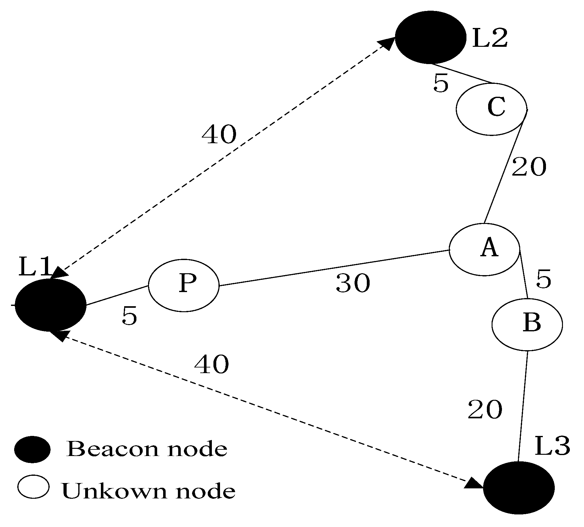
In DV-Hop, as long as the node receives packet from neighbor node, the hop count is 1 regardless of the distance, as shown in Figure 1. Although the distance between L1 and P, P and A is different, they are all recorded as 1 hop. There will certainly be large error if the minimum hops calculated in this way, which are used to continue the subsequent localization.

2.2.2. Error Caused by Hopsize

Since L1, L2, and L3 are beacon nodes and the coordinate positions of the three nodes are known, both of the real distances between L1 and L2 and L1 and L3 are calculated as 40 using the Euclidean distance. The path with the minimum number of hops from L1 to L2 passes through P, A and C nodes, respectively, so the minimum number of hops is 4. Similarly, the minimum number of hops from L1 to L3 is 4. According to the second step of the DV-Hop positioning process, $hopsize$ of L1 is calculated as $\frac{40+40}{4+4}=10$ by Formula (1). As L1 is the closest node of UN P, the $hopsize$ of L1 is taken as the $hopsize$ of UN P, and the estimated distance between L1 and UN P is $10\times 1=10$ while the actual distance is 5, so the error is large.

3. Related Research

The deployment scale of IoT equipment has grown rapidly in recent years. Many application fields need to obtain accurate location information of people and things. For location-based IoT services and indoor and outdoor integration positioning, academia and industry have conducted extensive exploration and practice. Satellite-based positioning systems are widely used in outdoor scenes, such as Beidou system, GPS system, etc.

However, the positioning accuracy of nodes widely distributed in the urban environment often decreases due to the obstruction of the building structure to the satellite signal. To resolve this problem, literature [25] improves the positioning accuracy of nodes by building a GPS signal network sharing multiple nodes in a single car, integrating the acceleration sensor and magnetometer in the user’s smartphone to predict the user’s trajectory, and estimating the relative distance between two nodes in a single car. Literature [26] designed a strategy to correct the original GPS observation information based on the reinforcement learning model, and achieved more stable positioning performance through an efficient confidence reward mechanism. In order to further improve the accuracy of satellite positioning and meet the needs of high-precision positioning in autopilot and other applications, Qianxun Location Network has achieved centimeter-level outdoor positioning precision degrees [27]. Literature [28] achieved a positioning accuracy of 0.2 m. This scheme requires complex sensors and high system computing power, resulting in high system power consumption and cost. Literature [29] designed an outdoor group-aware location method based on WiFi hotspots, which simplifies the structure of the location system and reduces the power consumption of nodes. Literature [30] designed an adaptive switching spatiotemporal fusion detection method, which realized the detection and positioning of small unmanned aerial vehicles in airspace through the image information observed by the electronic optical camera.

Unlike the outdoor scene, the indoor environment lacks a general positioning system due to the serious attenuation of satellite signals. In recent years, the academic and industrial circles have carried out research and application of indoor positioning through WiFi, RFID, Bluetooth, ultra-wideband (UWB), ultrasound and other means for node positioning in complex indoor environment. Reference [31] designed a fingerprint location method based on user-guided following strategy. However, such methods need to build corresponding fingerprint database for specific environment. In response to this problem, literature [32] designed an ultra-low load WiFi fingerprint map construction method, which reduced the cost of fingerprint database construction and extended the maintenance cycle. Literature [33] designed a fingerprint location method based on multi-user group intelligence perception, which solved the problem of fingerprint database construction to a certain extent. Literature [34] designed a privacy protection location method under the condition of ensuring accuracy to solve the problem of user privacy disclosure. Literature [35] proposed a three-dimensional indoor localization system based on a Bayesian graphical model which collected received signal strength indicators from each access point in an offline training phase and then estimated the user location in an online localization phase. Literature [36] proposed an application of the standard particle swarm optimization algorithm to Wi-Fi fingerprint-based indoor localization, wherein a new two-panel fingerprint homogeneity model is adopted to characterize fingerprint similarity.

4. The improved DV Hop Algorithm

4.1. Hop Correction Based on RSSI Ranging

Compared with the previous hop count method, the idea of multiple communication radii is adopted in literature [19], but the idea of multiple communication radii will greatly increase energy consumption of the node, and the accuracy of the hop count is directly related to the degree of division of the pre-propagation radius. The idea of two communication half paths is adopted in literature [20], which cannot make a more accurate division of the hops, and as the communication radius increases, the hop count becomes more and more inaccurate.

For this reason, this paper adopts the idea of RSSI ranging to divide hops continuously, making discrete hops become continuous hops. However, because RSSI is vulnerable to interference from environment, noise, multipath propagation and other factors, this paper first optimizes RSSI by weighted normal filtering, and uses the filtered distance to divide hops continuously.

4.1.1. RSSI Ranging Model

RSSI is now one of the most popular ranging algorithms, because most sensor chips now have the function of measuring RSSI strength, and it can complete the range estimation without adding any other additional hardware equipment to the sensor.

However, it is impossible to always carry out accurate ranging because RF signals are greatly affected by terrain, weather and human factors and because of the fluctuating characteristics of the received signal power, so the error of distance estimation based on transmission power loss is large. To avoid this problem, RSSI is introduced in this paper not to use it for ranging, but only as an auxiliary tool for hop thinning in DV-Hop algorithm. In this paper, the widely used Log Normal signal model is used to depict the relation between RSSI and space. Even in the environment with shelter, it can flexibly establish different expressions of signal attenuation and propagation distance. The model is expressed as

$$\left[\mathrm{P}{\left(\mathrm{d}\right)}_{\mathrm{dB}}\right]=\left[\mathrm{P}{\left({\mathrm{d}}_0\right)}_{\mathrm{dB}}\right]-10\mathsf{\gamma }\lg \left(\frac{\mathrm{d}}{{\mathrm{d}}_0}\right)+{\mathrm{X}}_{\sigma },$$

(2)

where $\mathrm{P}\left(\mathrm{d}\right)$ is the signal intensity at d from the transmission point, $\mathrm{P}\left({\mathrm{d}}_0\right)$ is the signal strength from the transmission point, which is the reference signal strength, generally taken as 1 m and its value is known, $\mathsf{\gamma }$ is the path loss index, and ${\mathrm{X}}_{\sigma }$ is Gaussian noise.

4.1.2. Weighted Normal Filtering

Because signals are often interrupted by environment, noise, multipath effect, etc., when they are transmitted, the signal value taken over by the node is often not the true value, but the interfered value. Therefore, this paper uses weighted normal distribution to process the signal value received by the sensors. The normal distribution is

$$\mathrm{f}\left(\mathrm{x}\right)=\frac{1}{\sqrt{2\mathsf{\pi }}\sigma }\exp \left(-\frac{{\left(\mathrm{x}-\mu \right)}^2}{2{\sigma }^2}\right),$$

(3)

$$\mu =\frac{1}{N}{\displaystyle \sum }_{i=1}^N{\mathrm{x}}_i,$$

(4)

$$\sigma =\sqrt{\frac{1}{N-1}{\displaystyle \sum }_{i=1}^N{\left(\mathrm{x}-\mu \right)}^2},$$

(5)

where, μ is the mean of signal, and $\sigma$ is the standard deviation of signal. According to the $3\sigma$ principle of normal distribution, the probability of signal distribution within the range $\left(\mu -\sigma ,\mu +\sigma \right)$ is 0.6526. In this paper, the value of $\mathrm{RSSI}$ within this range is taken as the effective value to avoid the impact of abnormal values on the overall value, and a series of effective values within this range are weighted and optimized.

Assume that a group of valid values filtered by the node are $({\mathrm{RSSI}}_1, {\mathrm{RSSI}}_2, \dots , {\mathrm{RSSI}}_{\mathrm{n}})$, and average them to obtain

$${\mathrm{RSSI}}_{\mathrm{a}}=\frac{1}{\mathrm{n}}\left({\mathrm{RSSI}}_1+{\mathrm{RSSI}}_2+\dots +{\mathrm{RSSI}}_{\mathrm{n}}\right).$$

(6)

The weight value is

$${\mathrm{w}}_i=\frac{1}{1+\left|{\mathrm{RSSI}}_i-{\mathrm{RSSI}}_{\mathrm{a}}\right|}.$$

(7)

The final ${\mathrm{RSSI}}_i^{\prime }$ is obtained through the following equation:

$${\mathrm{RSSI}}_i^{\prime }={\mathrm{w}}_i{\mathrm{RSSI}}_i.$$

(8)

After weighted normal processing, nodes can obtain more accurate RSSI values, which minimizes the impact of the external environment.

4.1.3. RSSI Ratio Correct Hops

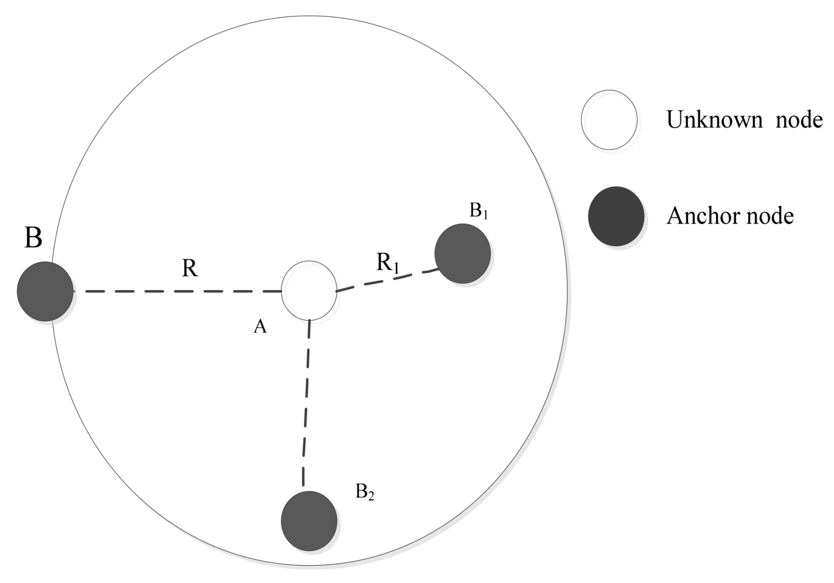
The node communication radius R is selected as the best one-hop distance, and hop is recorded as 1 when the space between the two nodes is R, then hops between two nodes are calculated by using the proportion of the true distance within the communication range and R. When there are nodes with unknown coordinates in adjacent nodes, the true distance cannot be obtained. However, all nodes have the functionality of gathering RSSI, so the RSSI value received by UNs can be used to quantify hops.

When the distance between two nodes is R, ${\mathrm{RSSI}}_{\mathrm{R}}$ is used to represent the received signal strength, and ${\mathrm{RSSI}}_{\mathrm{R}}$ is defined as the reference $\mathrm{RSSI}$ value. The ratio of $\mathrm{RSSI}$ value between neighbor nodes and reference $\mathrm{RSSI}$ are used as hops between two nodes.

Assuming $\mathrm{RSSI}$ received by node from the neighbor is ${\mathrm{RSSI}}_{\mathrm{k}}$, the hops from node K to the neighbor node are

$${hop}_i=\frac{{\mathrm{RSSI}}_{\mathrm{k}}}{{\mathrm{RSSI}}_{\mathrm{R}}}\le 1.$$

(9)

As shown in Figure 2, it is an abridged general view of hop quantization between two nodes. When $hop=1$, it means a node is on a circle with radius of communication radius, such as B. When $hop<1$, it means the distance between nodes A and B₁ is less than R, that is, at points B₁ and B₂ in Figure 2, the hops are less than 1.

The RSSI ranging technology is introduced to quantify the hops, serialize discrete hops, so the relative distance between actual nodes is more accurate, and make the distance estimation between two nodes more accurate.

4.2. Correct Hopsize

In DV-Hop, the $hopsize$ is important for reckoning the distance of nodes. The DV-Hop used unbiased estimation to calculate the $hopsize$, but this method failed to take into account that the error is stochastically distributed into positive and negative phases, leading to the minimization of the overall error, which cannot minimize all errors. Therefore, the MMSE criterion under the best index is used to count the $hopsiz{e}_{}$ and introduces the matching relationship between BN distance and hops to jointly amend it, to further reduce the error of it and improve the positioning effect.

The adaptive MMSE criterion is adopted to minimize the total error globally. Compared with the deviation and variance, it is more reasonable to apply it to the calculation of $hopsize$, but the fitness function must satisfy Formula (10):

$$\mathrm{f}=\frac{1}{N-1}{\displaystyle \sum }_{i\ne j}{(\sqrt{{\left({\mathrm{x}}_i-{\mathrm{x}}_j\right)}^2+{\left({\mathrm{y}}_i-{\mathrm{y}}_j\right)}^2}-{hopsize}_i\times {hop}_{ij})}^2,$$

(10)

where $({\mathrm{x}}_i,{\mathrm{y}}_i)$, $({\mathrm{x}}_j,{\mathrm{y}}_j)$ are the coordination positions of BNs $i$ and $j$, respectively, $N$ is the number of BNs, ${hopsize}_i$ is the average distance per hop of BNs $i$ and $j$, ${hop}_{ij}$ are the minimum hops between BNs $i$ and $j$.

In order to discuss the increment of hopsize, the partial derivative of the fitness function is obtained, and the other independent variables are constant, so the derivative is taken as 0.

$$\frac{\partial \mathrm{f}}{\partial hopsiz{e}_i}=0.$$

(11)

The $hopsiz{e}_i$ is calculated by Equation (12):

$$hopsiz{e}_i=\frac{{{\displaystyle \sum }}_{i\ne j}\left(\sqrt{{\left({\mathrm{x}}_i-{\mathrm{x}}_j\right)}^2+{\left({\mathrm{y}}_i-{\mathrm{y}}_j\right)}^2}\times {hop}_{ij}\right)}{{{\displaystyle \sum }}_{i\ne j}{hop}_{ij}{}^2}.$$

(12)

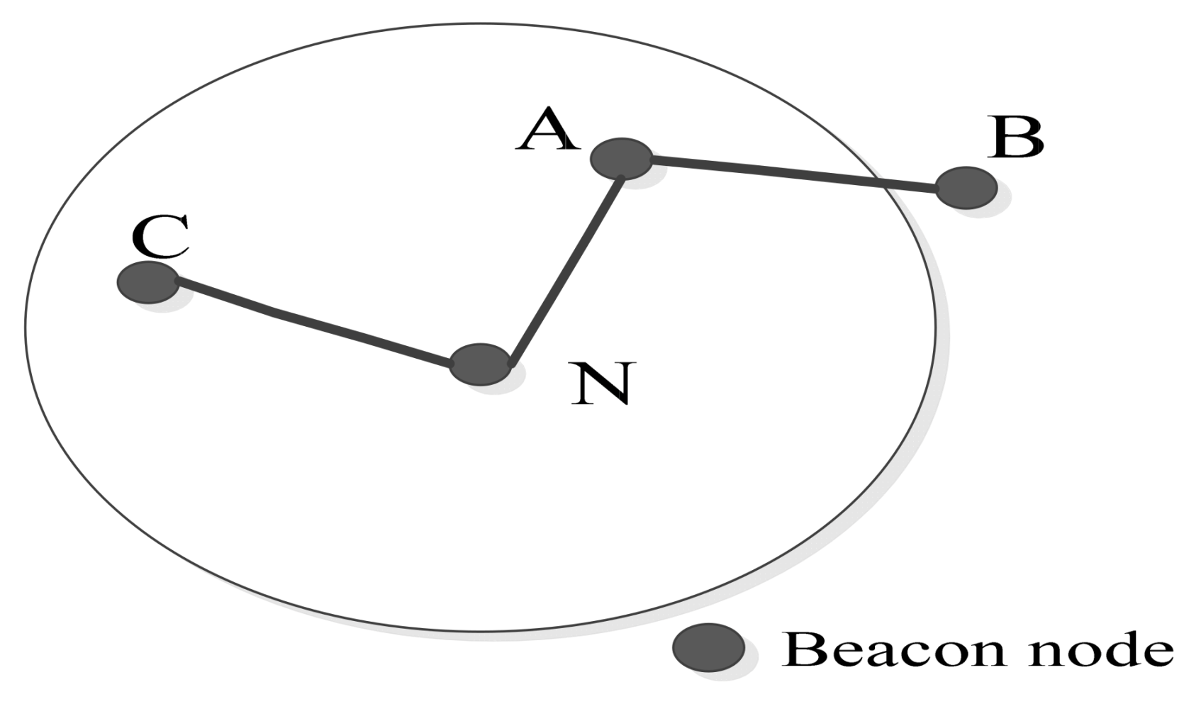
However, this fitness function does not take into account the matching relationship between the BN distance and hops when computing $hopsize$ of the BN, as shown in Figure 3.

All of the distances between beacon node N and beacon node A, beacon node N and beacon node B, beacon node N and beacon node C are approximately the node communication radius distance R. However, the hops between beacon node N and beacon node A, B and C are approximately ${hop}_{NA}$, ${hop}_{NA}+{hop}_{AB}$, ${hop}_{NC}$. If this beacon node relationship is viewed in the same way, there will be a large error when computing $hopsize$ of the beacon node. In this paper, the hop distance matching factor $\mathsf{\gamma }$ is used to modify the fitness function, where

$${\mathsf{\gamma }}_{ij}=\frac{\sqrt{{\left({\mathrm{x}}_i-{\mathrm{x}}_j\right)}^2+{\left({\mathrm{y}}_i-{\mathrm{y}}_j\right)}^2}}{{hop}_{ij}},$$

(13)

where $({\mathrm{x}}_i,{\mathrm{y}}_i)$, $({\mathrm{x}}_j,{\mathrm{y}}_j)$ are the coordination positions of BNs $i$ and $j$, respectively, ${hop}_{ij}$ are the minimum hops between BNs $i$ and $\mathrm{j}$.

This hop distance matching factor can make the weight value assigned to BNs with mismatched distance and hops smaller when calculating hop distance. As depicted in Figure 1, when calculating the $hopsize$ of BN N, the weights assigned to BNs A, B and C are

$${\mathsf{\gamma }}_{NA}=\frac{\sqrt{{\left({\mathrm{x}}_N-{\mathrm{x}}_A\right)}^2+{\left({\mathrm{y}}_N-{\mathrm{y}}_A\right)}^2}}{{hop}_{NA}},$$

(14)

$${\mathsf{\gamma }}_{NB}=\frac{\sqrt{{\left({\mathrm{x}}_N-{\mathrm{x}}_B\right)}^2+{\left({\mathrm{y}}_N-{\mathrm{y}}_B\right)}^2}}{{hop}_{NB}},$$

(15)

$${\mathsf{\gamma }}_{NC}=\frac{\sqrt{{\left({\mathrm{x}}_N-{\mathrm{x}}_C\right)}^2+{\left({\mathrm{y}}_N-{\mathrm{y}}_C\right)}^2}}{{hop}_{NC}},$$

(16)

where $({\mathrm{x}}_N,{\mathrm{y}}_N)$, $({\mathrm{x}}_A,{\mathrm{y}}_A)$, $({\mathrm{x}}_B,{\mathrm{y}}_B),({\mathrm{x}}_C,{\mathrm{y}}_C)$ are the coordination positions of nodes $N,A,B$ and $C$, respectively, ${hop}_{NA}, {hop}_{NB, }{hop}_{NC}$ are the minimum hops between nodes $N$ and A, nodes $N$ and B, nodes $N$ and C, respectively.

Therefore, the $hopsize$ is obtained by Equation (17):

$$\mathrm{f}=\frac{1}{N-1}{\displaystyle \sum }_{i\ne j}{\mathsf{\gamma }}_{ij}{}^2{(\sqrt{{\left({\mathrm{x}}_i-{\mathrm{x}}_j\right)}^2+{\left({\mathrm{y}}_i-{\mathrm{y}}_j\right)}^2}-{hopsize}_i\times {hop}_{ij})}^2.$$

(17)

In the same way, the partial derivative of fitness function is calculated and taken as 0.

$$\frac{\partial \mathrm{f}}{\partial hopsiz{e}_i}=0.$$

(18)

$hopsiz{e}_i$ is calculated as follows:

$$hopsiz{e}_i=\frac{{{\displaystyle \sum }}_{i\ne j}{\mathsf{\gamma }}_{ij}{}^2\times \left(\sqrt{{\left({\mathrm{x}}_i-{\mathrm{x}}_j\right)}^2+{\left({\mathrm{y}}_i-{\mathrm{y}}_j\right)}^2}\times {hop}_{ij}\right)}{{{\displaystyle \sum }}_{i\ne j}{\mathsf{\gamma }}_{ij}{}^2\times {hop}_{ij}{}^2}.$$

(19)

The deviation between the estimated distance and the true space is small in terms of the $hopsize$ calculated by Equation (19). In addition, this paper introduces the changed exponential value $\mathsf{\theta }$ into Equation (19) above. According to the influence of different values on the positioning error, the best value is selected to apply to the correction of $hopsize$. Equation (20) is rewritten as follows:

$${hopsize}_{\mathrm{i}}=\frac{{{\displaystyle \sum }}_{i\ne j}{\mathsf{\gamma }}_{ij}{}^2\times \left(\sqrt{{\left({\mathrm{x}}_i-{\mathrm{x}}_j\right)}^2+{\left({\mathrm{y}}_i-{\mathrm{y}}_j\right)}^2}\times {hop}_{ij}\right)}{{{\displaystyle \sum }}_{i\ne j}{\mathsf{\gamma }}_{ij}{}^2\times {hop}_{ij}{}^{\mathsf{\theta }}}.$$

(20)

4.3. Correct Coordination Position of UN

In terms of the quantized hops recorded by the UN and the modified $hopsize$, the estimated coordinates of the UN can be obtained. The space between the estimated coordinates and the real coordinates to each BN is different. To lessen the computation, only the distance discrepancy between the estimated coordinates and the real coordinates to the nearest BN of the UN is taken into account. In fact, the distance between the estimated coordinates to the nearest BN of the UN and should be the same as the space between the real coordinates to the nearest BN of the UN, so the estimated coordinates should be correct to meet the reality.

Because RSSI ranging technology can accurately estimate the space between two nodes that are close to each other, the RSSI value is applied to estimate the distance between the UN and the nearest BN, and the distance is regarded as the veritable distance between them.

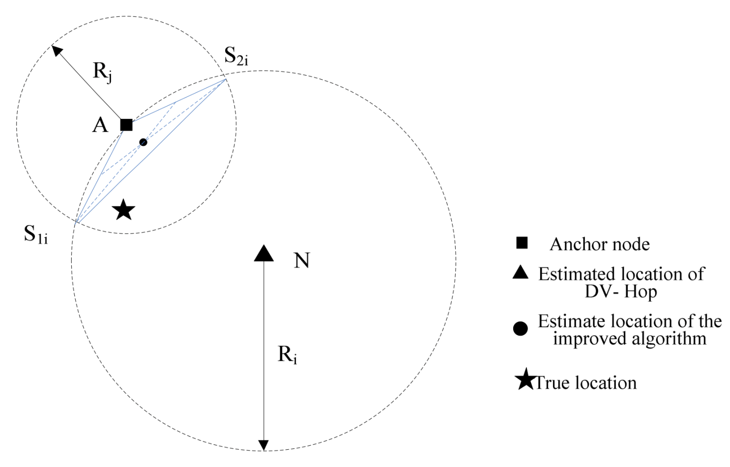
Assume that the coordinates of A are estimated to be $\left({\mathrm{x}}_{\mathrm{e}},{\mathrm{y}}_{\mathrm{e}}\right)$ by using the modified $hopsize$ of UN A and the consecutive hops to each BN, and the distance between the estimated coordinates and the nearest BN B$\left({\mathrm{x}}_{\mathrm{B}},{\mathrm{y}}_{\mathrm{B}}\right)$ is $\mathrm{d}=\sqrt{{\left({\mathrm{x}}_{\mathrm{B}}-{\mathrm{x}}_{\mathrm{e}}\right)}^2+{\left({\mathrm{y}}_{\mathrm{B}}-{\mathrm{y}}_{\mathrm{e}}\right)}^2}$. RSSI ranging technology is used to estimate the distance between A and the nearest BN as ${\mathrm{d}}_{\mathrm{n}}$, and whether to correct the estimated coordinates of A is determined by comparing whether $\mathrm{d}$ and ${\mathrm{d}}_{\mathrm{n}}$ are the same. Let the modified coordination be $\left({\mathrm{x}}_{\mathrm{m}},{\mathrm{y}}_{\mathrm{m}}\right)$, and the purpose of the modification is to make the distance from the modified coordination to the nearest BN of A equal to the distance from A to the nearest BN. To modify the estimated coordinates on the line is the best way, and the modified result of the estimated coordinates of node A can be obtained through of Equation (21):

$$\{\begin{array}{c}{\mathrm{x}}_{\mathrm{i}}={\mathrm{x}}_{\mathrm{e}}+\left({\mathrm{x}}_{\mathrm{B}}-{\mathrm{x}}_{\mathrm{e}}\right)\times \frac{\mathrm{d}-{\mathrm{d}}_{\mathrm{n}}}{\mathrm{d}}\\ {\mathrm{y}}_{\mathrm{i}}={\mathrm{y}}_{\mathrm{e}}+\left({\mathrm{y}}_{\mathrm{B}}-{\mathrm{y}}_{\mathrm{e}}\right)\times \frac{\mathrm{d}-{\mathrm{d}}_{\mathrm{n}}}{\mathrm{d}}\end{array}.$$

(21)

Because DV-Hop location algorithm assumes that the location is carried out in the regular network topology structure, the location error increases in the irregular network structure, while most of the practical applications are irregular network structures. In order to obtain good location accuracy, this paper makes a secondary correction to the UN coordinates obtained. The BN A with the minimum hops originating from the UN is selected, and its coordination position is marked as $({\mathrm{x}}_{\mathrm{j}},{\mathrm{y}}_{\mathrm{j}})$. A circle is drawn with UN N and BN A as the center, ${\mathrm{R}}_{\mathrm{i}}$, ${\mathrm{R}}_{\mathrm{j}}$ as the radius, as shown in Figure 4. where ${\mathrm{R}}_i=\sqrt{{\left({\mathrm{x}}_i-{\mathrm{x}}_j\right)}^2+{\left({\mathrm{y}}_i-{\mathrm{y}}_j\right)}^2}$, ${\mathrm{R}}_j=\mathrm{HS}\prime \times {hop}_{ij}$.

The intersection of two circles ${\mathrm{S}}_{1i}\left({\mathrm{x}}_{1i},{\mathrm{y}}_{1i}\right)$,${\mathrm{S}}_{2i}\left({\mathrm{x}}_{2i},{\mathrm{y}}_{2i}\right)$ is determined. The triangle’s centroid obtained by the two intersection points and the BN is the coordination position of the UN. The final UN coordination position is calculated by Equation (22):

$${\mathrm{X}}_i^{\mathrm{t}}\left({\mathrm{x}}_{\mathrm{t}},{\mathrm{y}}_{\mathrm{t}}\right)=\left(\frac{{\mathrm{x}}_{i+}{\mathrm{x}}_{1i+}{\mathrm{x}}_{2i}}{3},\frac{{\mathrm{y}}_{i+}{\mathrm{y}}_{1i+}{\mathrm{y}}_{2i}}{3}\right).$$

(22)

5. Simulation Results and Discussion

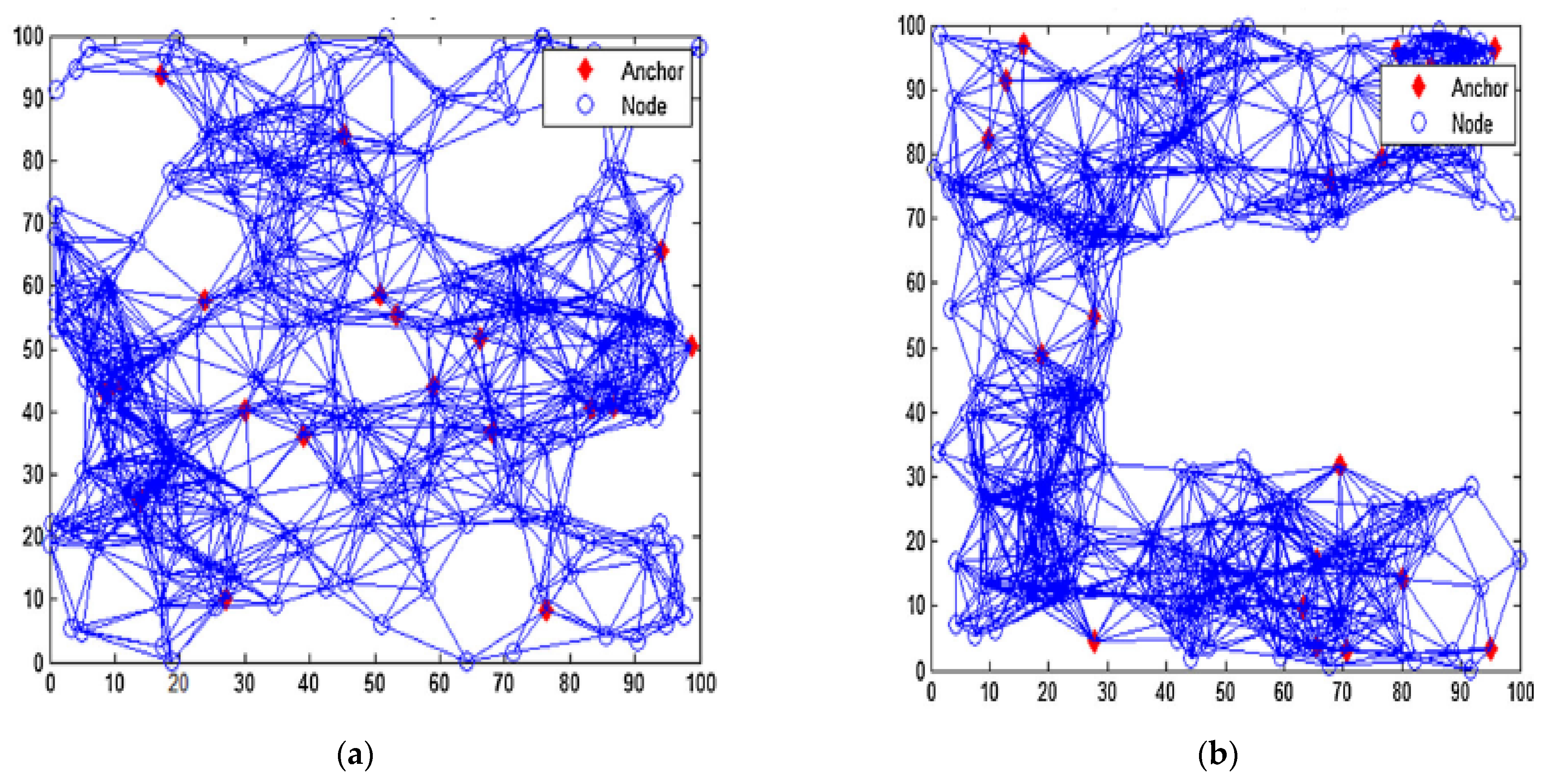
To evaluate the performance of the proposed algorithm, all experiments are designed to be simulated on the MATLAB platform. In the uniform random network and C-type random network, as depicted in Figure 5a,b, the nodes are stochastically fixed up in the square area, and the localization deviation is used as the evaluation index of this experiment. We assume that the real coordinates and estimated coordinates of UNs are $\left({\mathrm{x}}_{\mathrm{t}},{\mathrm{y}}_{\mathrm{t}}\right),\left({\mathrm{x}}_{\mathrm{e}},{\mathrm{y}}_{\mathrm{e}}\right),$ respectively, the communication radius is R, the sum of nodes is N, the number of BNs is M, and the localization error is defined as

$$\mathrm{err}=\frac{{{\displaystyle \sum }}_{i=1}^{\mathrm{N}-\mathrm{M}}\sqrt{{\left({\mathrm{x}}_{\mathrm{e}}-{\mathrm{x}}_{\mathrm{t}}\right)}^2+{\left({\mathrm{y}}_{\mathrm{e}}-{\mathrm{y}}_{\mathrm{t}}\right)}^2}}{\mathrm{R}\times \left(\mathrm{N}-\mathrm{M}\right)}.$$

(23)

The proposed algorithms, the algorithm in literature [21] (Improved DV-Hop1), literature [22] (Improved DV-Hop2), literature [23] (Improved DV-Hop3)and DV-Hop algorithm are run:

Figure 5. (a) Uniform random network; (b) C-type random network.

Figure 5. (a) Uniform random network; (b) C-type random network.

5.1. Simulation Results for the Uniform Random Network

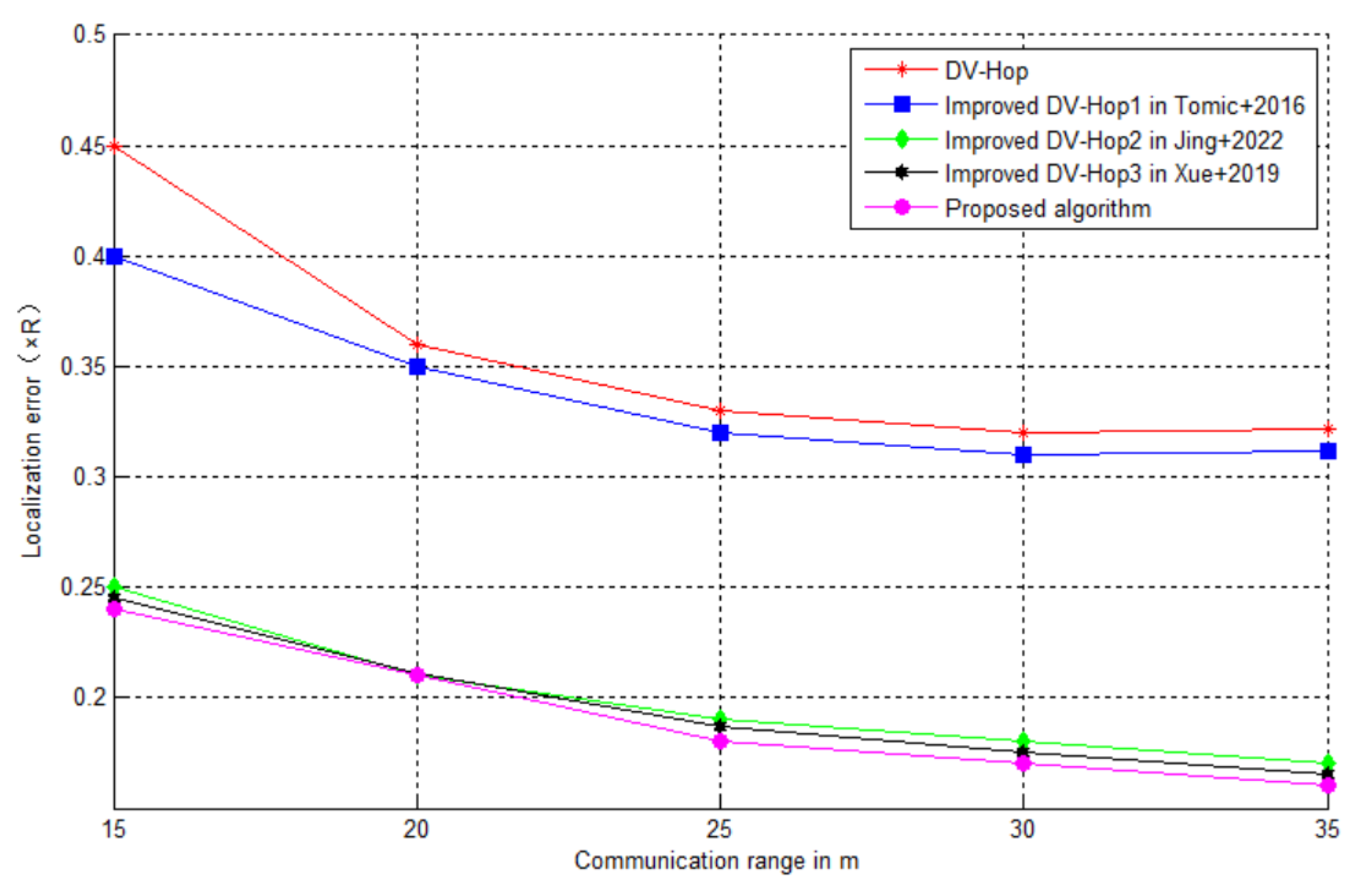
In a uniform random network environment, 200 UNs are stochastically distributed, the sum of nodes is fixed, the percentage of BNs is 10%, and R of nodes is changed. The traditional DV-Hop is run, improved DV-Hop1, improved DV-Hop2, improved DV-Hop3 and the improved algorithm proposed in this paper are run separately. Figure 6 depicts the results.

Figure 6 shows that DV-Hop1 only revised the coordination of UNs, DV-Hop2, DV-Hop3 and the new algorithm all revised the minimum hops and $hopsize$ between two nodes, reducing the estimated distance deviation between UNs and BNs, so their localization errors are lower than those of the traditional DV-Hop and DV-Hop1. With communication range R = 15 m, the proposed DV-Hop has an approximate 0.24 R localization error while DV-Hop has an approximate 0.45 R error and DV-Hop1 has an approximate 0.4 R error, and DV-Hop2 and DV-Hop3 also show better performance with approximate 0.25 R and 0.245 R localization errors, respectively. In the uniform network structure environment, the positioning deviation of the new algorithm is slightly higher than that of DV-Hop2 and DV-Hop3, as it corrects the UNs coordinates.

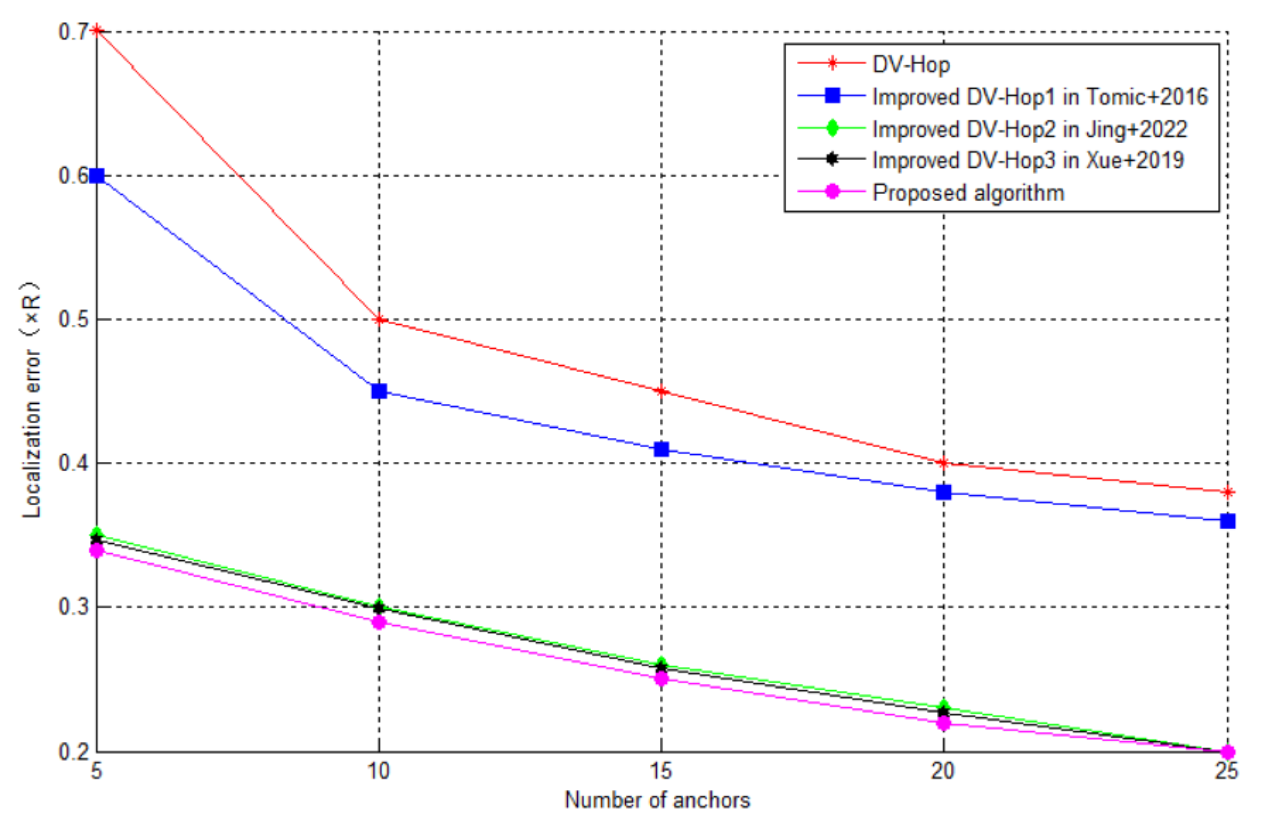
The sum of all nodes is unchanged, R = 15 m, and the proportion of BNs is changed. The four algorithms are then run separately. Figure 7 depicts the simulation results.

Figure 7 depicts that the localization deviation of the five algorithms lessen when the proportion of BNs aggrandizes, but the localization precision of the new algorithm and the DV-Hop2 and DV-Hop3 is obviously better than that of DV-Hop and DV-Hop1. The average localization errors of DV-Hop2, DV-Hop3 and the proposed DV-Hop are approximately 0.27 R, 0.27 R and 0.26 R, respectively. The errors of DV-Hop and DV-Hop1 are approximately 0.49 R and 0.41 R, respectively. The proposed DV-Hop has the lowest localization error compared to other algorithms for scenario with five anchors.

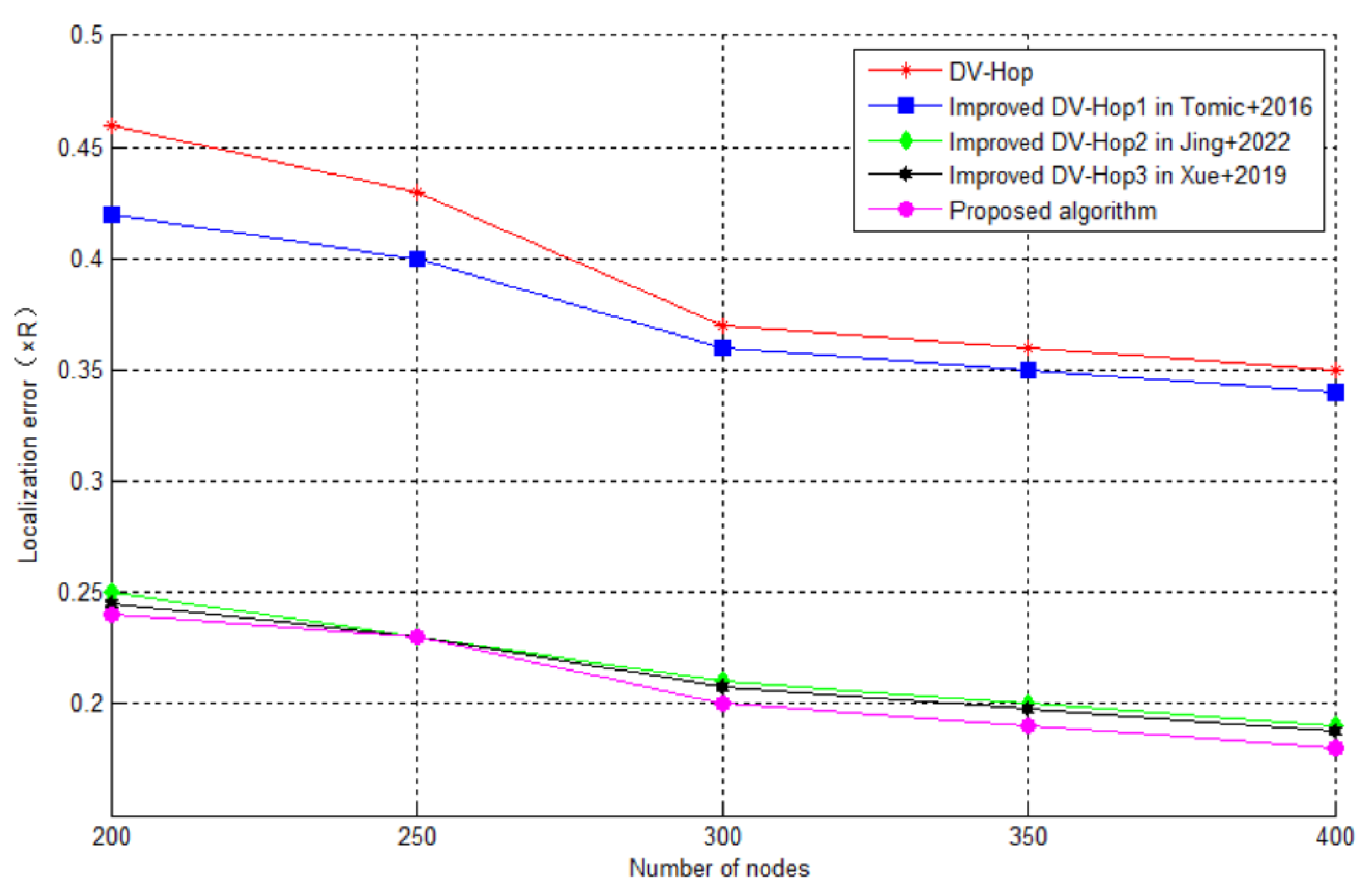
The number of nodes is 200, 250, 300, 350, 400, with R = 15 m, and the ratio of BNs is 10%. The five algorithms are run separately. The simulation results are shown in Figure 8.

Figure 8 shows that as the average number of neighbors per node increases (that is, the network density increases), the localization deviation of the five algorithms lessens when the proportion of BNs enlarges. However, the localization precision of the new algorithm and the improved DV-Hop2 and improved DV-Hop3 algorithms is much better than that of DV-Hop and the improved DV-Hop1. The new algorithm depicts the best performance, with the lowest average localization error at approximately 0.21 R. Compared to the improved DV-Hop2 and DV-Hop3, average localization error is lower by approximately 7% and approximately 6%. Compared to the improved DV-Hop1 and DV-Hop, average localization error of the proposed in the paper is lower by approximately 47% and 43%.

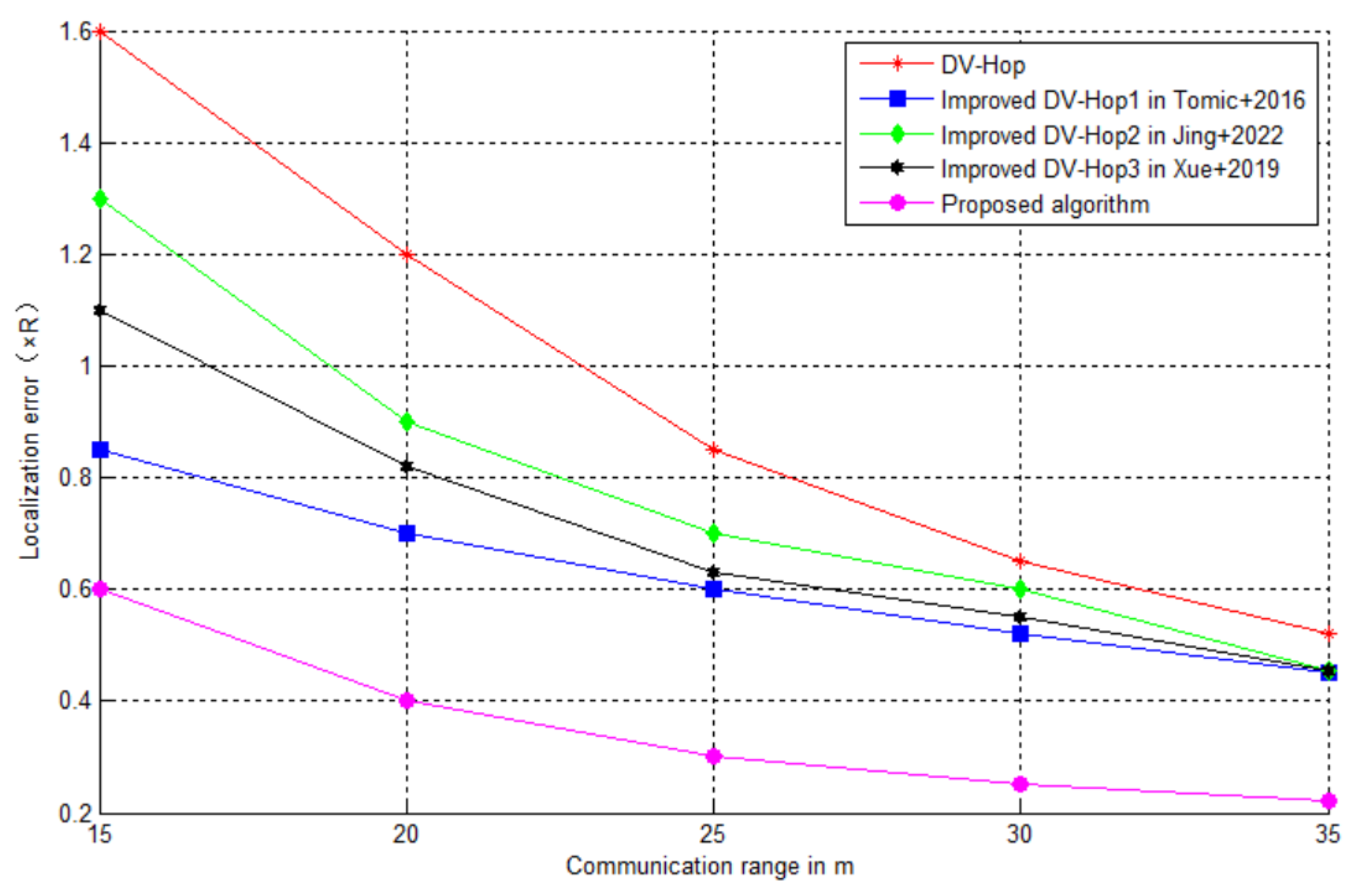
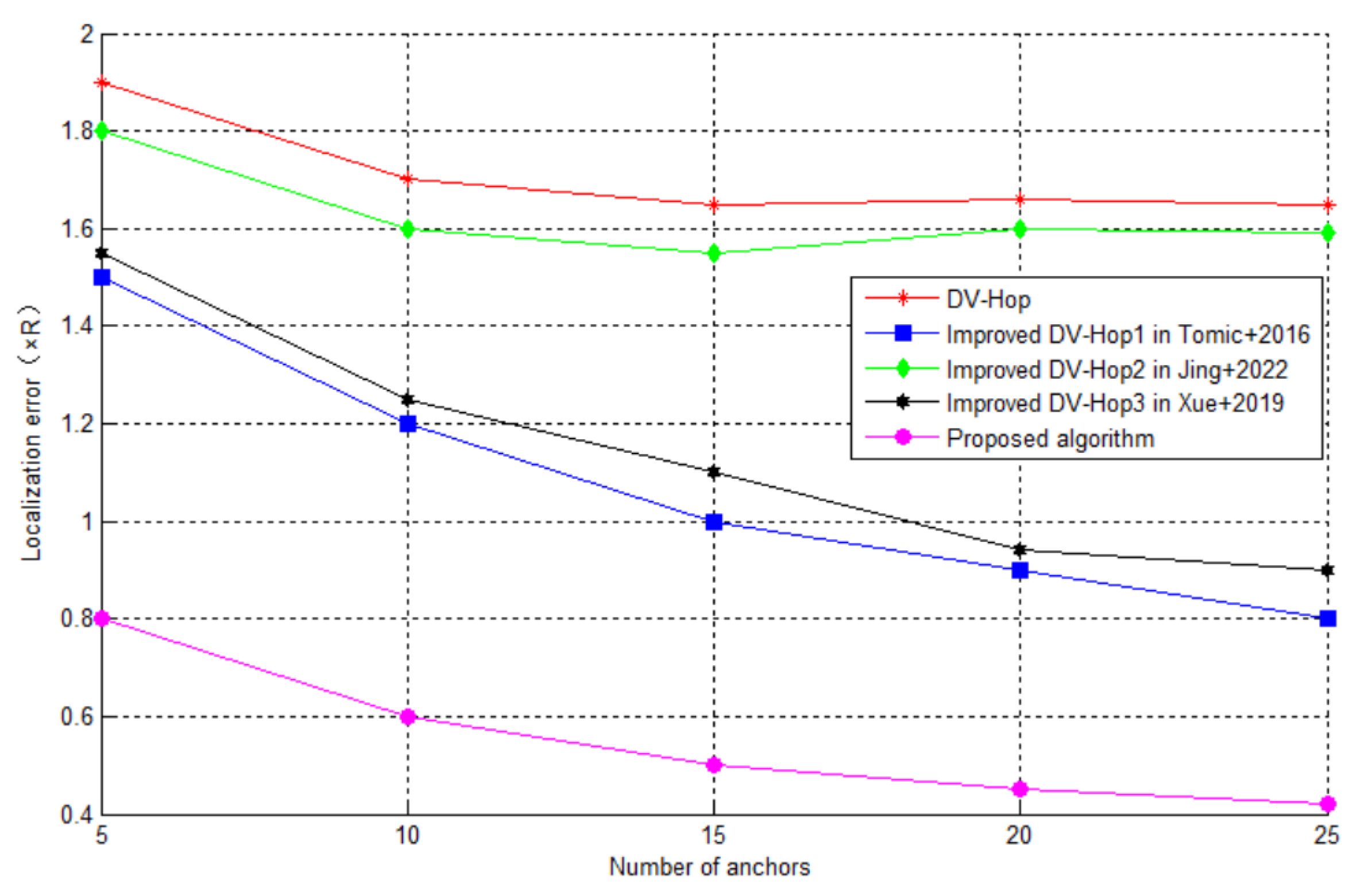
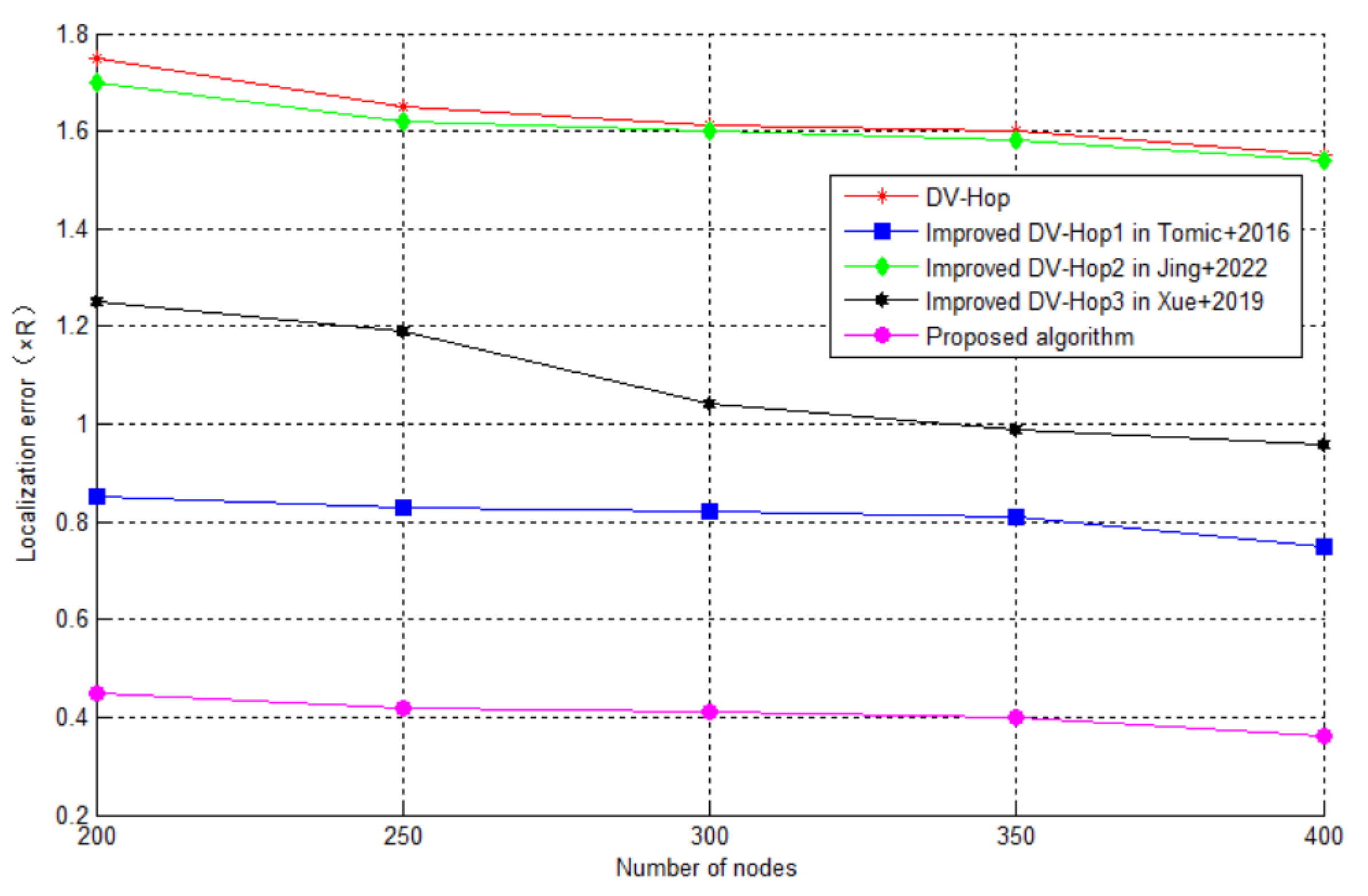
5.2. Simulation Results of C-Shaped Random Network

In the C-type random network environment, the sum nodes are kept unchanged and R is changed. The sum of nodes is kept unchanged, the proportion of BNs and the number of nodes are changed, and the proportion of BNs is unchanged. The five positioning algorithms are run. The simulation results are shown in Figure 9, Figure 10 and Figure 11. The figures show that in the non-uniform network environment, the positioning deviation of DV-Hop and the improved DV-Hop2, DV-Hop3 is larger than that in the uniform network environment. However, since the new algorithm and the improved DV-Hop1 have modified the coordinates of UNs, it can still be effectively located in the non-uniform network. Compared to the improved DV-Hop2 and DV-Hop3, average localization error is lower by approximately 60% and approximately 51%. Compared to the improved DV-Hop1 and DV-Hop, average localization error of the one proposed in the paper is lower by approximately 68% and 44%.

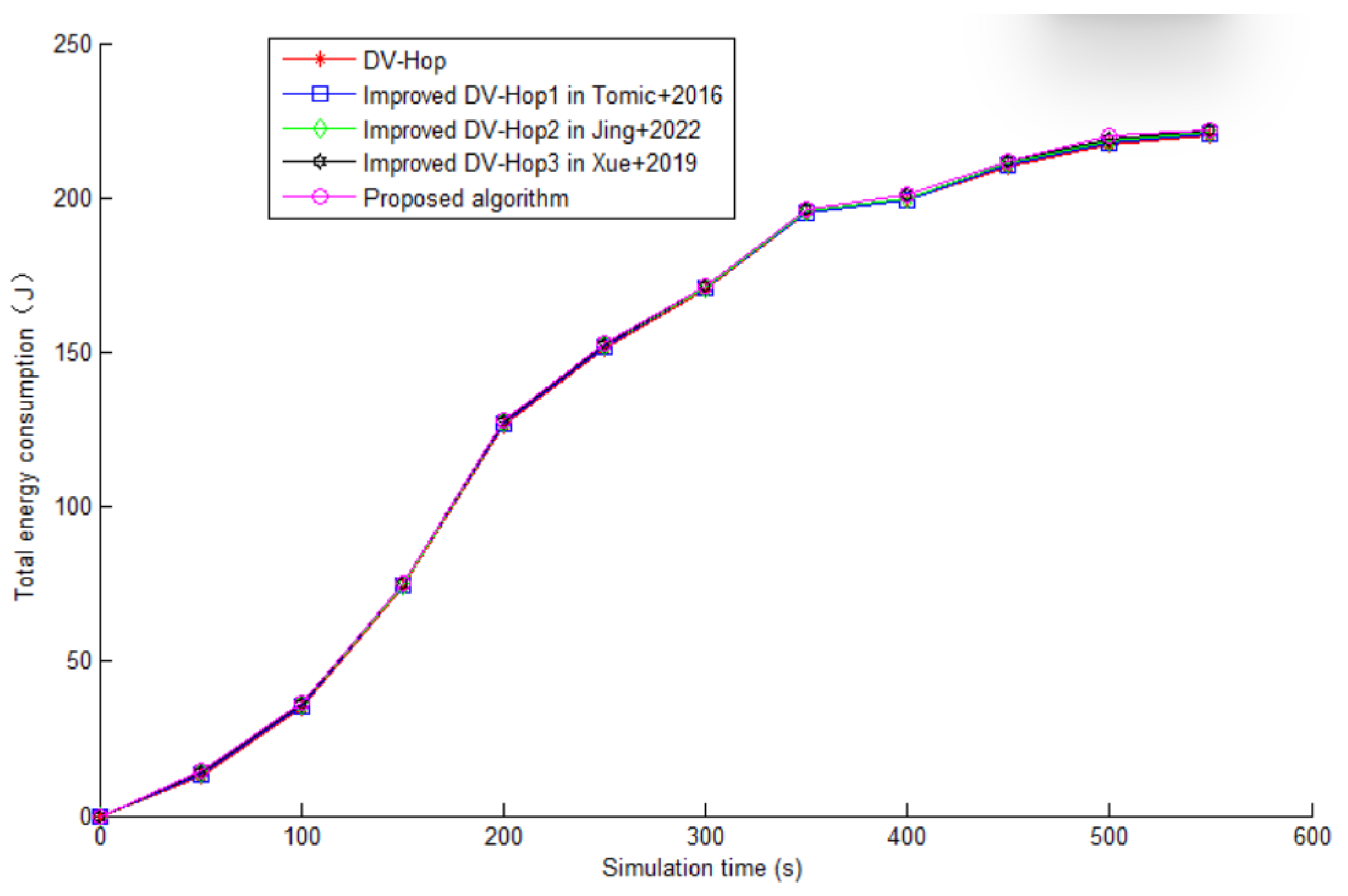
5.3. Comparison of Energy Utilization Efficiency of Algorithms

When the simulation time of the five algorithms is the same, the comparison of total energy consumption is shown in Figure 12. It can be seen from the figure that the energy consumption of the algorithm proposed in this paper is slightly higher than that of the other three algorithms, but it is not very obvious. This is due to the fact that in the positioning process, the improved algorithm optimizes the hops and the average distance per hop and corrects the coordinate position of unknown node twice, which constitutes part of the energy consumption. In wireless sensor networks with limited energy, it is of great significance to achieve higher positioning accuracy with little energy consumption.

6. Conclusions

DV-Hop has low localization precision. Because the hop number of 1 has the greatest impact on node location, the new DV-Hop put forward in this paper hierarchically processes the hop number of 1 to make it closer to the actual hop number. In addition, DV-Hop uses unbiased estimation to calculate the jump distance. When the overall error is minimized, it fails to minimize various errors. Therefore, this paper uses the square error function as the fitness function to solve the jump distance, and the original algorithm does not consider the matching relationship between the hops and the distance in the process of calculating $hopsize$ of the BN, which introduces more errors. Therefore, the hop distance matching factor is proposed to weigh the fitness of each BN and introduce the change index value, so as to obtain more accurate $hopsize$, which effectively improves the localization precision of the algorithm. Finally, the UNs can still be located effectively in the irregular network by modifying their estimated positions twice.

References

- Prasannababu, D.; Amgoth, T. Joint mobile wireless energy transmitter and data collector for rechargeable wireless sensor networks. Wirel. Netw. 2022, 28, 3563–3576. [Google Scholar] [CrossRef]
- Ghafour, M.G.A.E.; Kamel, S.H.; Abouelseoud, Y. Improved DV-Hop based on Squirrel search algorithm for localization in wireless sensor networks. Wirel. Netw. 2021, 27, 2743–2759. [Google Scholar] [CrossRef]
- Wang, R.B.; Wang, W.F.; Xu, L.; Pan, J.S.; Chu, S.C. Correction to: Improved DV-Hop based on parallel and compact whale optimization algorithm for localization in wireless sensor networks. Wirel. Netw. 2022, 28, 3429. [Google Scholar] [CrossRef]
- Cao, Y.; Wang, Z. Improved DV-Hop Localization Algorithm Based on Dynamic Anchor Node Set for Wireless Sensor Networks. IEEE Access 2019, 7, 124876–124890. [Google Scholar] [CrossRef]
- Fu, S.; Lou, W.; Wang, J.; Ji, T.; Liu, W. Multi-barycenter Nodes Localization Method in Wireless Sensor Network Based on Improved RSSI. J. Beijing Inst. Technol. 2021, 30, 210–217. [Google Scholar] [CrossRef]
- Lyu, Y.; Mo, Y.; Yue, S.; Liu, W. Improved Beetle Antennae Algorithm Based on Localization for Jamming Attack in Wireless Sensor Networks. IEEE Access 2022, 10, 13071–13088. [Google Scholar] [CrossRef]
- Pan, J.S.; Wang, J.; Lai, J.; Lai, J.; Luo, H.; Chu, S.-C. A Modes Communication of Cat Swarm Optimization Based WSN Node Location Algorithm. J. Internet Technol. 2021, 22, 949–956. [Google Scholar] [CrossRef]
- Sabale, K.; Mini, S. Localization in Wireless Sensor Networks with Mobile Anchor Node Path Planning Mechanism. Inf. Sci. 2021, 579, 648–666. [Google Scholar] [CrossRef]
- Zhang, Y.; Jiang, J.; Zhang, G.; Lu, Y. Accurate and Robust Synchronous Extraction Algorithm for Star Centroid and Nearby Celestial Body Edge. IEEE Access 2019, 7, 126742–126752. [Google Scholar] [CrossRef]
- Liu, G.; Qian, Z.; Wang, X. An improved DV-Hop localization algorithm based on hop distances correction. China Commun. 2019, 16, 200–214. [Google Scholar] [CrossRef]
- Tang, F.; Pedrycz, W. An improved DV-Hop algorithm based on differential simulated annealing evolution. Int. J. Sens. Netw. 2022, 38, 1–11. [Google Scholar] [CrossRef]
- Pan, J.S.; Gao, M.; Li, J.P.; Chu, S.C. A compact GBMO applied to modify DV-Hop based on layers in a wireless sensor network. Int. J. Ad Hoc Ubiquitous Comput. 2022, 39, 20–36. [Google Scholar] [CrossRef]
- Han, D.; Wang, J.; Tang, C.; Weng, T.; Li, K.; Dobre, C. A multi-objective distance vector-hop localization algorithm based on differential evolution quantum particle swarm optimization. Int. J. Commun. Syst. 2021, 34, e4924.1–e4924.17. [Google Scholar] [CrossRef]
- Shi, Q.; Wu, C.; Xu, Q.; Zhang, J. Optimization for DV-Hop type of localization scheme in wireless sensor networks. J. Supercomput. 2021, 77, 13629–13652. [Google Scholar] [CrossRef]
- Shi, Q.; Xu, Q.; Zhang, J. Amended DV-hop scheme based on N-gram model and weighed LM algorithm. Electron. Lett. 2020, 56, 247–250. [Google Scholar] [CrossRef]
- Mohanta, T.K.; Das, D.K. Improved Wireless Sensor Network Localization Algorithm Based on Selective Opposition Class Topper Optimization (SOCTO). Wirel. Pers. Commun. 2022, 80, 529–543. [Google Scholar] [CrossRef]
- Cai, X.; Wang, P.; Cui, Z.; Zhang, W.; Chen, J. Weight convergence analysis of DV-hop localization algorithm with GA. Soft Comput. 2020, 24, 18249–18258. [Google Scholar] [CrossRef]
- Messous, S.; Liouane, H.; Liouane, N. Improvement of DV-Hop localization algorithm for stochastically deployed wireless sensor networks. Telecommun. Syst. 2020, 73, 75–86. [Google Scholar] [CrossRef]
- Peng, D.; Yang, Y.; Gao, Y.; Wang, C. Node location algorithm based on multiple communication radii and sparrow search. J. Sens. Technol. 2021, 34, 1523–1529. [Google Scholar] [CrossRef]
- Li, T.; Wang, C.; Na, Q. Research o DV-Hop improved algorithm based on dual communication radius. EURASIP J. Wirel. Commun. Netw. 2020, 113. [Google Scholar] [CrossRef]
- Tomic, S.; Mezei, I. Improvements of DV-Hop localization algorithm for wireless sensor networks. Telecommun. Syst. Model. Anal. Des. Manag. 2016, 61, 93–106. [Google Scholar] [CrossRef]
- Jing, Z.; Yu, L. Improved three-time correction DV-Hop positioning algorithm. J. Chin. Comput. Syst. 2022, 43, 1762–1768. [Google Scholar]
- Xue, D. Research of localization algorithm for wireless sensor network based on DV-Hop. J. Wirel. Commun. Netw. 2019, 2019, 2–8. [Google Scholar] [CrossRef] [Green Version]
- Niculescu, D.; Nath, B. Ad HocPositioning System(APS). In Proceedings of the IEEE Global Telecommunications Conference, San Francisco, CA, USA, 30 March–3 April 2003; pp. 2926–2931. [Google Scholar] [CrossRef]
- Chen, K.; Tan, G. BikeGPS: Localizing shared bikes in street canyons with low level GPS cooperation. ACM Trans. Sens. Netw. 2019, 15, 1–28. [Google Scholar] [CrossRef]
- Zhang, E.; Masoud, N. Increasing GPS localization accuracy with reinforcement learning. IEEE Trans. Intell. Transp. Syst. 2020, 22, 2615–2626. [Google Scholar] [CrossRef]
- Qianxun Location Network Co., Ltd. RTK. Available online: https://www.qxwz.com (accessed on 1 December 2022).
- Schaupp, L.; Pfreundschuh, P.; Burki, M.; Cadena, C.; Siegwart, R.; Nieto, J. MOZARD: Multi modal localization for autonomous vehicles in urban outdoor environments. In Proceedings of the 2020 IEEE/RSJ International Conference on Intelligent Robots and Systems, Las Vegas, NV, USA, 24 October 2020–24 January 2021; pp. 4828–4833. [Google Scholar] [CrossRef]
- Wang, J.; Luo, J.; Pan, S.J.; Sun, A. Learning based outdoor localization exploiting crowd labeled WiFi hotspots. IEEE Trans. Mob. Comput. 2019, 18, 896–909. [Google Scholar] [CrossRef]
- Xie, J.; Yu, J.; Wu, J.; Shi, Z.; Chen, J. Adaptive switching spatial temporal fusion detection for remote flying drones. IEEE Trans. Veh. Technol. 2020, 69, 6964–6976. [Google Scholar] [CrossRef]
- Zhang, Z.; He, S.; Shu, Y.; Shi, Z. A self evolving Wi Fi-based indoor navigation system using smartphones. IEEE Trans. Mob. Comput. 2019, 19, 1760–1774. [Google Scholar] [CrossRef]
- Jun, J.; He, L.; Gu, Y.; Jiang, W.; Kushwaha, G.; Vipin, A.; Cheng, L.; Liu, C.; Zhu, T. Low -Overhead Wi-Fi Fingerprinting. IEEE Trans. Mob. Comput. 2018, 17, 590–603. [Google Scholar] [CrossRef]
- Zhuang, Y.; Syed, Z.; Li, Y.; El-Sheimy, N. Evaluation of two WiFi positioning systems based on autonomous crowdsourcing of handheld devices for indoor navigation. IEEE Trans. Mob. Comput. 2016, 15, 1982–1995. [Google Scholar] [CrossRef]
- Yang, Z.; Järvinen, K. The death and rebirth of privacy preserving WiFi fingerprint localization with paillier encryption. In Proceedings of the 37th Annual IEEE International Conference on Computer Communications, Honolulu, HI, USA, 16–19 April 2018; pp. 1223–1231. [Google Scholar] [CrossRef] [Green Version]
- Alhammadi, A.; Hashim, F.; A Rasid, M.F.; Alraih, S. A three-dimensional pattern recognition localization system based on a Bayesian graphical model. Int. J. Distrib. Sens. Netw. 2020, 16(9), 1–11. [Google Scholar] [CrossRef]
- Zheng, J.; Li, K.; Zhang, X. Wi-Fi Fingerprint-Based Indoor Localization Method via Standard Particle Swarm Optimization. Sensors 2022, 22, 5051. [Google Scholar] [CrossRef] [PubMed]
Figure 1.
Error Analysis.
Figure 2.
Hop quantization between nodes.
Figure 3.
Distribution diagram of beacon nodes.
Figure 4.
Correction of UN coordination position.
Disclaimer/Publisher’s Note: The statements, opinions and data contained in all publications are solely those of the individual author(s) and contributor(s) and not of MDPI and/or the editor(s). MDPI and/or the editor(s) disclaim responsibility for any injury to people or property resulting from any ideas, methods, instructions or products referred to in the content. |
© 2023 by the authors. Licensee MDPI, Basel, Switzerland. This article is an open access article distributed under the terms and conditions of the Creative Commons Attribution (CC BY) license (https://creativecommons.org/licenses/by/4.0/).
Share and Cite
MDPI and ACS Style
Zhang, W.; Yang, X. DV-Hop Location Algorithm Based on RSSI Correction. Electronics 2023, 12, 1141. https://doi.org/10.3390/electronics12051141
AMA Style
Zhang W, Yang X. DV-Hop Location Algorithm Based on RSSI Correction. Electronics. 2023; 12(5):1141. https://doi.org/10.3390/electronics12051141
Chicago/Turabian StyleZhang, Wanli, and Xiaoying Yang. 2023. "DV-Hop Location Algorithm Based on RSSI Correction" Electronics 12, no. 5: 1141. https://doi.org/10.3390/electronics12051141
Note that from the first issue of 2016, this journal uses article numbers instead of page numbers. See further details here.