Article

A Hybrid STA Based on Nelder–Mead Simplex Search and Quadratic Interpolation

School of Automation, Central South University, Changsha 410083, China
*
Author to whom correspondence should be addressed.
Electronics 2023, 12(4), 994; https://doi.org/10.3390/electronics12040994
Submission received: 15 January 2023 / Revised: 6 February 2023 / Accepted: 11 February 2023 / Published: 16 February 2023

Abstract

:
State transition algorithm (STA) is a metaheuristic method for global optimization. However, due to the insufficient utilization of historical information, it still suffers from slow convergence speed and low solution accuracy on specific problems in the later stages. This paper proposes a hybrid STA based on Nelder–Mead (NM) simplex search and quadratic interpolation (QI). In the exploration stage, NM simplex search utilizes the historical information of STA to generate promising solutions. In the exploitation stage, QI utilizes the historical information to enhance the local search capacity. The proposed method uses an eagle strategy to maximize the efficiency and stability. The proposed method successfully combines the merits of the three distinct approaches: the powerful exploration capacity of STA, the fast convergence speed of NM simplex search and the strong exploitation capacity of QI. The hybrid STA is evaluated using 15 benchmark functions with dimensions of 20, 30, 50 and 100. Moreover, the results are statistically analyzed using the Wilcoxon signed-rank sum test. In addition, the applicability of the hybrid STA to solve real-world problems is assessed using the wireless sensor network localization problem. Compared with six state-of-the-art metaheuristic methods, the experimental results demonstrate the superiority and effectiveness of the proposed method.

Graphical Abstract

1. Introduction

With the increasing complexity of practical problems, global optimization plays a significant role in many real-world applications, including engineering design, manufacturing system, economics, physical science, machine learning and other related fields [1]. Due to the difficulty and inefficiency in finding the global extremum using traditional optimization methods, metaheuristics can be a practical and elegant method to provide a satisfactory solution to practical engineering optimization problems [2].
Metaheuristic methods have been classified into different literary categories, such as evolutionary-based algorithms, swarm-based algorithms, physics-based algorithms and hybrid algorithms. Evolutionary-based methods originate from the theory of evolution, such as genetic algorithms [3] and differential evolution [4]. In recent years, there have been many effective and competitive evolutionary-based algorithms, including QANA [5] and DMDE [6]. Swarm-based algorithms emulate the collective decision-making of various social groups. Particle swarm optimization (PSO) [7,8,9] is an excellent classical swarm-based algorithm.
PSO has many attractive advantages, such as its simple implementation and fewer controlling parameters. Thus, it is widely applied in feature selection, wireless communications, image processing, electrical power systems and other fields [10]. Physics-based algorithms are inspired by the laws of natural physics. Simulated annealing [11], gravitational search algorithm (GSA) [12] and artificial electric field optimization [13] are classical and popular physics-based methods. Furthermore, hybrid algorithms combine several methods to obtain better results.
The state transition algorithm (STA) [14,15] is a novel metaheuristic method for global optimization that was proposed in recent years. Different from many popular population-based metaheuristic methods, such as PSO and artificial bee colony (ABC) [16,17], STA is an individual-based metaheuristic method. The basic idea of STA is to regard a solution as a state, and the update of a solution can be considered as a state transition.
When solving an optimization problem, state transformation operators of STA are adopted alternately, and then the candidate solution set is generated by a sampling technique. Finally, the incumbent best solution is updated by a selection criterion. Due to the local and global search capabilities of the state transformation operators of STA, it has been successfully applied in many engineering problems, such as PID controller design [18,19], image segmentation [20], nonlinear system identification [21], feature selection [22,23], wind power forecasting [24,25] and other industrial applications [26,27,28,29].
Recently, a modified STA, named parameter optimized state transition algorithm (POSTA), was proposed in [30]. Based on a statistical study, POSTA provides a parameter selection mechanism to select the optimal parameters for the expansion operator, rotation operator and axesion operator in STA. Using appropriate operator parameters, POSTA has better solution accuracy and stronger global exploration ability than does STA. However, the historical information in POSTA is not sufficiently utilized. As a result, POSTA still suffers from slow convergence speed and low solution accuracy on specific problems in the later stage when facing complex high-dimensional global optimization problems.
To speed up the convergence during the whole search process in STA, Nelder–Mead (NM) simplex search [31,32] was introduced. NM simplex search is a classical direct search method with a fast convergence speed. The NM simplex is a geometric figure consisting of n + 1 vertices in n-dimensional space, which is able to store the information of n + 1 historical solutions in STA.
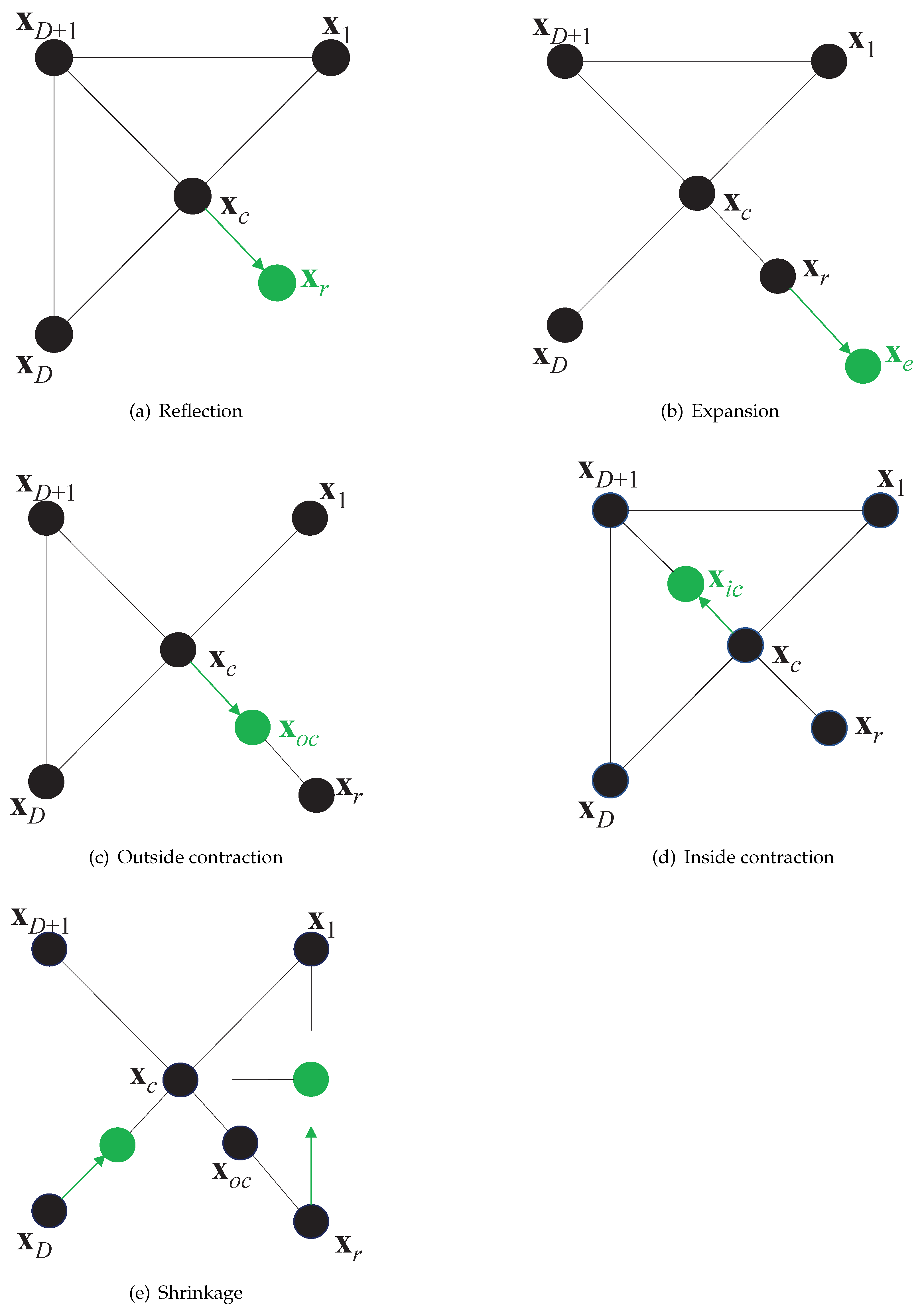
The operators in the NM method consist of a sequence of distinct geometric transformations (reflection, contraction...), which is able to utilize the historical information in STA. For decades, combining NM simplex search with metaheuristic methods has been a potential way to speed up the convergence [33,34]. However, few existing studies have used NM simplex search as a way to utilize the historical information. In this paper, a hybrid method is proposed by applying NM simplex search to make use of the historical information in STA.
To further improve the solution accuracy in later stages of the search, a quadratic interpolation (QI) strategy is also introduced in the hybrid STA. QI is a classical local search method and is widely used [35,36,37,38]. In QI, three known points are used as the search agents to generate a quadratic curve. The generated curve is seen as an approximate shape of the target function. To make full use of the historical information in later stages of the search, three historical solutions of STA are selected as the QI search agents to generate a new analytical solution with low computing cost. To a certain extent, QI can efficiently strengthen the exploitation capacity of STA.
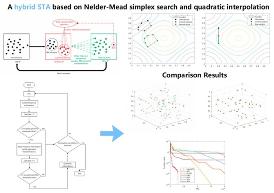
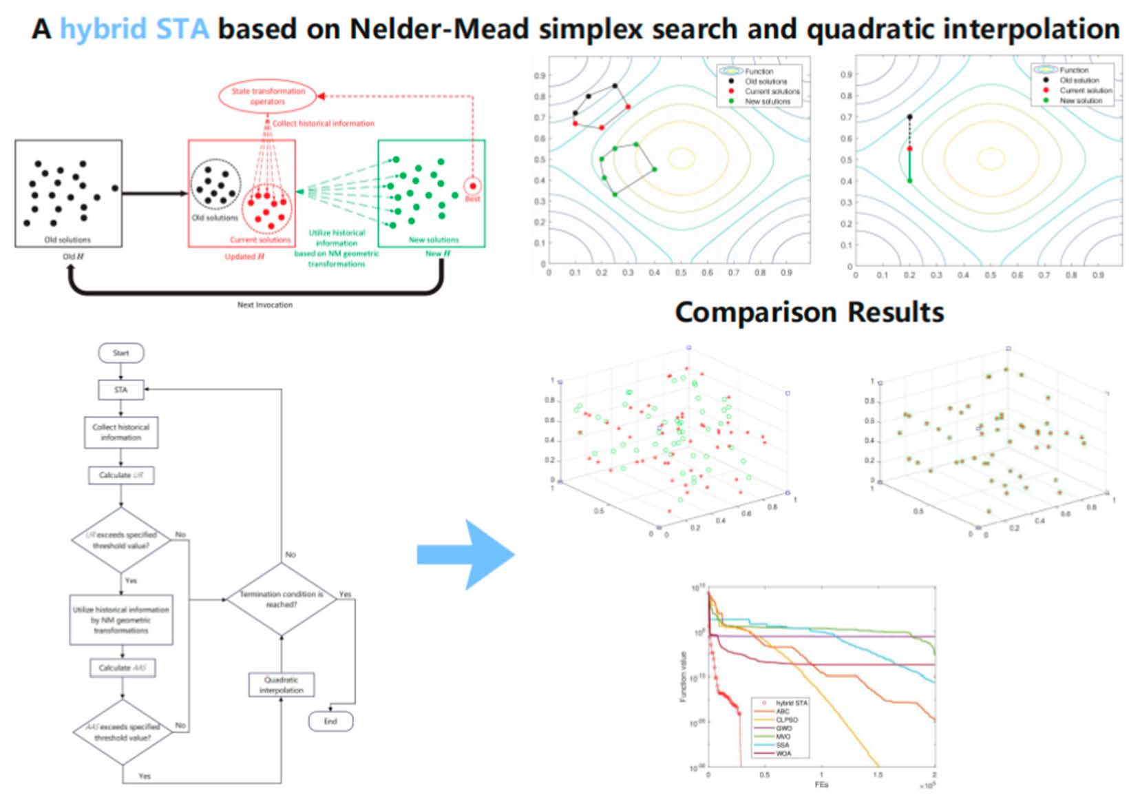
In summary, to make full use of the historical information in STA in different stages of search, a hybrid STA based on NM simplex search and QI is proposed in this study. Compared to STA, the hybrid STA overcomes the shortcoming of low convergence speed in the later stage of the search and has a perfect performance in both benchmark functions and practical problems. The main contributions of this paper can be summarized as follows:
(1) An efficient hybrid STA is proposed that successfully combines the merits of three distinct methods: the wide exploration capacity of STA, the fast convergence speed of NM simplex search and the strong exploitation capacity of QI.
(2) NM simplex search is adopted innovatively to utilize historical information for a faster convergence speed.
(3) The superiority and the effectiveness of the hybrid STA are verified by comparing six competitive metaheuristic methods with the STA family on 15 benchmarks and the wireless sensor network localization problem.
The remainder of the article is organized as follows. In Section 2, the algorithmic background of STA, NM simplex search and QI is reviewed. In Section 3, the proposed hybrid STA based on NM simplex search and QI is presented in detail. In Section 4, the proposed method is compared with six competitive metaheuristic methods and the STA family on 15 benchmark functions to demonstrate its efficiency and stability. In Section 5, hybrid STA is applied in the wireless sensor network localization problem to illustrate its ability to solve engineering problems.

2. Background

2.1. Brief Review of STA

STA is a novel metaheuristic method for global optimization. In STA, a solution can be regarded as a state, and the update of a solution can be seen as a state transition. In STA, based on state space representation, the general form of generating a solution is described as:
s k + 1 = A k s k + B k u k
where s k and s k + 1 are the current best state and the next state; A k and B k are state transition matrices, which can be to construct operators of the optimization algorithm; and u k is a function of s k and the historical states.

2.1.1. State Transformation Operators

(1) Rotation transformation
s k + 1 = s k + α 1 n s k 2 R r s k
where α is a positive parameter named the rotation factor; R r R D × D stands for a random matrix, and all its elements are distributed in the range of [−1,1]; and · 2 is the Euclidean-norm of a vector. The rotation transformation is capable of generating candidate solutions in a hypersphere with a maximum radius of α and is designed for local searches.
(2) Translation transformation
s k + 1 = s k + β R t s k s k 1 s k s k 1 2
where β is a positive constant named the translation factor; and R t R stands for a random variable, and all its elements belong to the range of [0,1]. The translation transformation has the function of searching along a line from x k 1 to x k at the starting point x k with the maximum length of β .
(3) Expansion transformation
s k + 1 = s k + γ R e s k
where γ is a positive parameter named the expansion factor; and R e R D × D is a random diagonal matrix with its entries obeying the standard normal distribution. The expansion transformation is able to search for solutions in the entire search space and is designed to strengthen the capacity of global searches.
(4) Axesion transformation
s k + 1 = s k + δ R a s k
where δ is a positive parameter named the axesion factor; and R a R D × D is a random diagonal matrix with its entries obeying the Gaussian distribution and only one random position with a nonzero value. The axesion transformation is designed to strengthen the single-dimensional search.

2.1.2. Parameter Selection Mechanism

According to a statistical study [30], the parameter of STA is a crucial factor for the performance. To simplify the selection of the parameter, the candidate values for all transformation factors are taken from the set Ω = { 1 , 1 × 10 1 , 1 × 10 2 , 1 × 10 3 , 1 × 10 4 , 1 × 10 5 , 1 × 10 6 , 1 × 10 7 , 1 × 10 8 }. Then, the value that leads to the optimal objective function value is chosen as the optimal value for further search. If the optimal parameter is denoted as a ˜ , the following formula represents the parameter selection. In Equation (7), α , γ , δ , 1 n s k 2 R r s k , R e s k and R a s k are parameters and variables in state transformation operators, and these are explained in detail in Section 2.1.1.
a ˜ = arg min a ˜ k Ω f s k + a ˜ k d ˜ k
1 n s k 2 R r s k R e s k R a s k d ˜ k , α γ δ a ˜ k .

2.1.3. Algorithm Procedure

To make full use of the optimal parameter, the selected optimal value is kept for a period of time that is denoted as T p . Specifically, the detailed procedures of the STA are as follows Algorithm 1:
Algorithm 1 Pseudocode of the STA
1:
repeat
2:
 Best ← expansion_w(objfun, Best, SE, Ω )
3:
 Best ← rotation_w(objfun, Best, SE, Ω )
4:
 Best ← axesion_w(objfun, Best, SE, Ω )
5:
until certain criterion is met
where objfun indicates the objective function, SE indicates the number of candidate solutions in the candidate solution set and Best indicates the current best solution. rotation_w(·) in the above pseudocode is given a detailed explanation Algorithm 2:
Algorithm 2 Pseudocode of rotation_w(·)
1:
 [Best, α ] ← update_ α (objfun, Best, SE, Ω )
2:
for each i [ 1 , T p ]  do
3:
    Best ← rotation(objfun, Best, SE, Ω )
4:
end for
where rotation(·) represents the invocation of the rotation operator and update_ α (·) represents the selection of optimal value for rotation factor α . The parameter selection for the expansion factor and axesion factor are similar to that for rotation factor. More details of STA can be found in [30].

2.2. Nelder–Mead Simplex Search

Nelder–Mead simplex search is a popular direct search method [39] with a fast convergence speed. The idea of NM simplex search focuses on a changeable simplex that approaches and approximates the optimum. For a D-dimensional function, it first initializes a simplex with D + 1 vertices and iteratively replace the worst vertex with a better one.
As shown in Figure 1, The new vertices in this process are generated by five geometric transformations, namely reflection, expansion, outside contraction, inside contraction and shrinkage. The detailed steps in NM simplex search are as follows:
Step 0: Initialization. Starting from an original point x 0 in D-dimensional space, the first simplex is generated by creating tiny perturbations in each dimension of x 0 with a rate of 0.25%. Specifically, the remaining D vertices are generated as:
x i = x 0 + τ i e i
τ i = 0.05 , if x 0 i 0 0.00025 , if x 0 i = 0
where i = 1 , , D + 1 , x 0 i is the component of x 0 in the i-th dimension and e i is the unit vector in the i-th dimension.
Step 1: Sorting. The vertices x i , i = 1 , , D + 1 are sorted and relabeled so that the function values are:
f x 1 f x 2 f x D + 1
Step 2: Reflection. Compute the reflection vertex x r as:
x r = x c + η x c x D + 1
where x c = i = 1 D x i / D and η is the reflection coefficient. If f x 1 f x r < f x D , then replace x D + 1 with x r .
Step 3: Expansion. If f x r < f x 1 , then compute the expansion vertex x e as:
x e = x c + λ x r x c
where λ is the expansion coefficient. If f x e < f x r , then replace x D + 1 with x e , else with  x r .
Step 4: Outside Contraction (OC). If f x D f x r < f x D + 1 , then compute the OC vertex x oc as:
x o c = x c + μ x r x c
where μ is the contraction coefficient. If f x o c f x r , then replace x D + 1 with x o c , else go to step 6.
Step 5: Inside Contraction (IC). If f x r f x D + 1 , then compute the IC vertex x i c  as:
x i c = x c μ x r x c
where μ is the contraction coefficient. If f x i c < f x D + 1 , then replace x D + 1 with x i c , else go to step 6.
Step 6: Shrinkage. For 2 i D + 1 , compute the vertex x i as:
x i = x 1 + ν x i x 1
where ν is the shrinkage coefficient.
Step 7: If the termination condition is satisfied, then stop, else go to step 1.

2.3. Quadratic Interpolation

QI is an analytical local search method that utilizes a parabola to fit the shape of the objective function. This method is capable of strengthening the exploitation capacity. In QI, three known points are used as the QI search agents to generate a quadratic curve, the generated quadratic curve is used as the approximate shape of the objective function, and the extreme point of the quadratic function can be used to approximate the optima of the objective function [40]. Theoretically, when the the QI search agents are close enough to the global minimum, the shape of the objective function can be well-approximated by the generated quadratic curve.
x d Q I = 0.5 ( x d b e s t ) 2 ( x d b ) 2 f x a + ( x d a ) 2 ( x d b e s t ) 2 f x b + ( x d b ) 2 ( x d a ) 2 f x b e s t x d b e s t x d b f x a + x d a x d b e s t f x b + x d b x d a f x b e s t , d = 1 , 2 , , D
For a D-dimensional problem, three QI search agents ( x a , x b and x b e s t ) are selected to generate a new solution x Q I . Suppose that
x a = x 1 a , x 2 a , , x D a ,
x b = x 1 b , x 2 b , , x D b ,
x b e s t = x 1 b e s t , x 2 b e s t , , x D b e s t
are the three distinct search agents; then, the new solution
x Q I = x 1 Q I , x 2 Q I , , x D Q I
can be calculated by using Equation (16), where f x a , f x b and f x b e s t are the fitness values of the three search agents, respectively. As a strong local search method, QI is capable of strengthening the exploitation capacity but could easily lead to a local minimum. Therefore, QI should only be invoked in a later stage of the search.

3. Proposed Hybrid Method

3.1. NM-STA

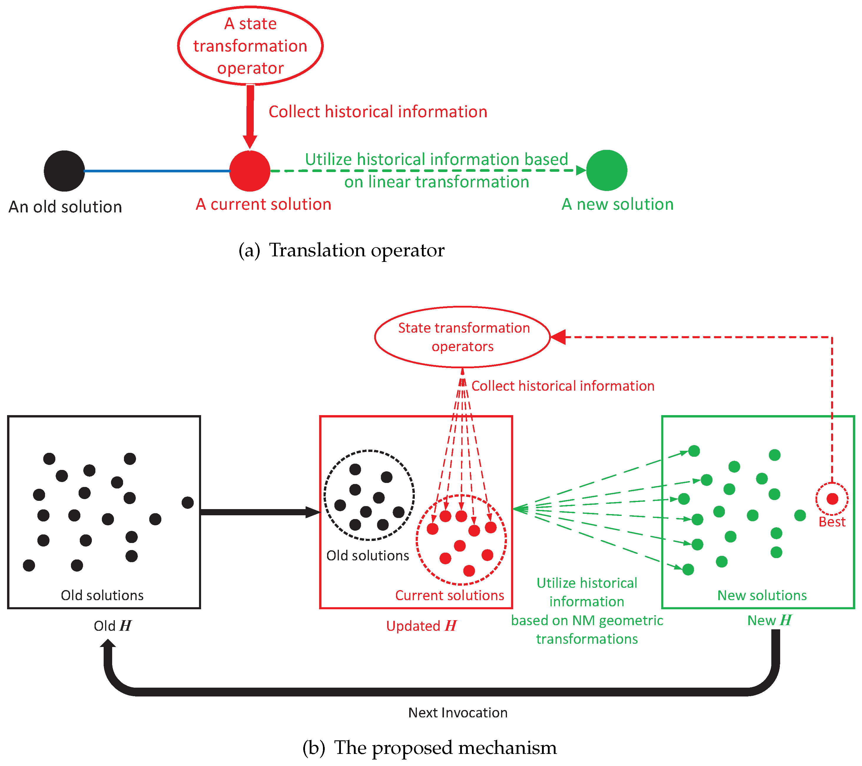
In traditional STA, the historical information is not utilized sufficiently. As shown in
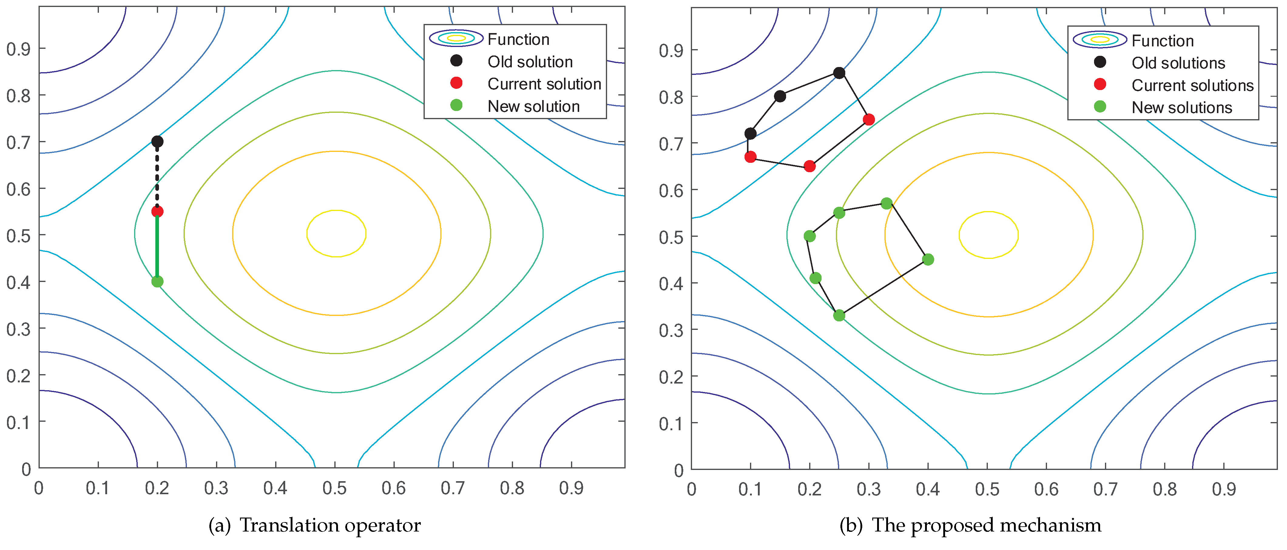
 Figure 2a and Figure 3a, the historical information is utilized by a translation operator. However, only the latest two historical solutions are collected, and only a linear search is applied to utilize the information. This inefficiency leads to the low convergence speed of STA on specific problems.
In past decades, combining NM simplex search with metaheuristic methods has been a popular way to speed up convergence. The general combination strategies between NM simplex search and metaheuristic methods can be summarized into two types: the staged pipelining type combination and the eagle strategy type combination [41]. In the first type, NM simplex search is applied to the superior individuals in the population [42]. In the second type, NM simplex search is applied in the exploitation stage as a local search method [33,43]. However, none of the existing combinations have seen NM simplex search as a way to utilize the information of historical solutions.
In this section, a hybrid STA with NM simplex search (NM-STA) is proposed. In NM-STA, a historical information mechanism based on NM simplex search is proposed to make use of the historical information. In the proposed mechanism, the historical information is collected based on a collection strategy, stored in the NM simplex and then utilized by the NM geometric transformations. The detailed historical information mechanism in NM-STA is illustrated as follows.

3.1.1. The Historical Information Set

In NM-STA, a historical information set called H is used to store the historical solutions generated by the state transformation operators. H has the capacity to store the coordinates of D + 1 vertices in D-dimensional space. Therefore, H can be seen as an NM simplex. For a D-dimensional problem, H is capable of storing the information of D + 1 historical solutions.
The historical information contained in H is more sufficient than that in the translation operator. As shown in Figure 2 and Figure 3, H contains information about a set of old solutions and a set of current solutions, but only an old solution and a current solution are considered in the translation operator.

3.1.2. Utilization of the Historical Information

In NM-STA, the NM geometric transformations are applied for utilization. As shown in Figure 1, the operators in the NM method consist of a sequence of distinct geometric transformations, which are more comprehensive than the linear transformation in the translation operator. As a result, NM-STA is able to utilize the historical information more comprehensively as shown in Figure 2 and Figure 3.
The detailed steps of utilizing historical information in NM-STA are illustrated in Algorithm 3. When Algorithm 3 is invoked, H is input as the initial simplex. After that, the NM geometric transformations are applied to the initialized simplex. In the inner iterations, the NM geometric transformations are run D + 1 times.
Algorithm 3 Utilize historical information based on NM geometric transformations
Input: 
Updated historical information set H
Output: 
New historical information set H , B e s t
1:
initial simplex ← H
2:
for each i [ 1 , D + 1 ]  do
3:
    NM geometric transformations
4:
end for
5:
H ← new simplex
6:
B e s t ← best solution in H
Considering that each iteration of NM geometric transformations approximately produces a new vertex, running D + 1 times approximately produces a new simplex with D + 1 new vertices. Therefore, a new simplex with D + 1 new vertices is generated, and they are then stored in H . As shown in Figure 3b, the new H contains D + 1 new solutions, and the top solution in H is denoted as B e s t . B e s t is then sent to the state transformation operators as the input of the current best solution.

3.1.3. Collection of Historical Information

An appropriate collection strategy of historical information is proposed to provide more promising input for utilization. Overall, the historical information is collected based on the collection strategy, stored in H and utilized by the NM geometric transformations. The utilization of historical information in NM-STA is illustrated in Algorithm 3. If an invocation of utilization is terminated, then the historical information needs to be re-collected before next utilization. Therefore, between the invocations of utilization, a collection strategy for historical information is considered.
In the collection strategy, two type of solutions are considered: old solutions and current solutions. As shown in Figure 3b, old solutions are the solutions generated in the last invocation of utilization. After the termination of the last utilization, the state transformation operators begin to generate solutions based on B e s t . Between the invocations of utilization, those solutions generated by STA are considered as current solutions.
This collection strategy is seen as an extended version of that in the translation operator. As shown in Figure 2a and Figure 3a, the translation operator uses an old solution and a current solution as the historical information. In NM-STA, a set of old solutions and a set of current solutions are used as the historical information as shown in Figure 2b and Figure 3b.
The collection strategy is implemented by updating H . As shown in Algorithm 4, a current solution x c u r r e n t is used to update H in an invocation. In the implementation, Algorithm 4 is invoked iteratively to update H with multiple current solutions. As shown in Figure 3b, H is updated by multiple current solutions before been utilized. To control the ratio between old solutions and current solutions in H , a parameter named the update rate (UR) is proposed:
U R = n c s n o s + n c s
where n o s and n c s are, namely, the number of old solutions and the number of current solutions in H . U R is calculated after each update, and only when U R exceeds a certain threshold value will the utilization be invoked.
Algorithm 4 Collect historical information.
Input: 
Old historical information set H , current solution x c u r r e n t
Output: 
Updated historical information set H
1:
replace the worst solution in H with x c u r r e n t
2:
return updated H

3.2. Properties of NM-STA

In this section, the fast convergence of NM-STA is briefly illustrated by a comparison between NM-STA and STA. To illustrate the effect of utilizing historical information, one classical test function is used, namely Rosenbrock (F7). NM-STA and STA are tested against the function in 2-D space, and each method is only terminated when a certain criterion is satisfied. After termination, the corresponding number of function evaluations (FEs) is recorded. For both STA and NM-STA, S E is set to 50, and T p is set to 10. In NM-STA, the threshold value for U R is set to 0.5, and the parameters in the NM simplex search are set as η , λ , μ , ν = 1 , 2 , 0.5 and 0.5 , which are the same as in the standard implementation of an NM simplex search [31].
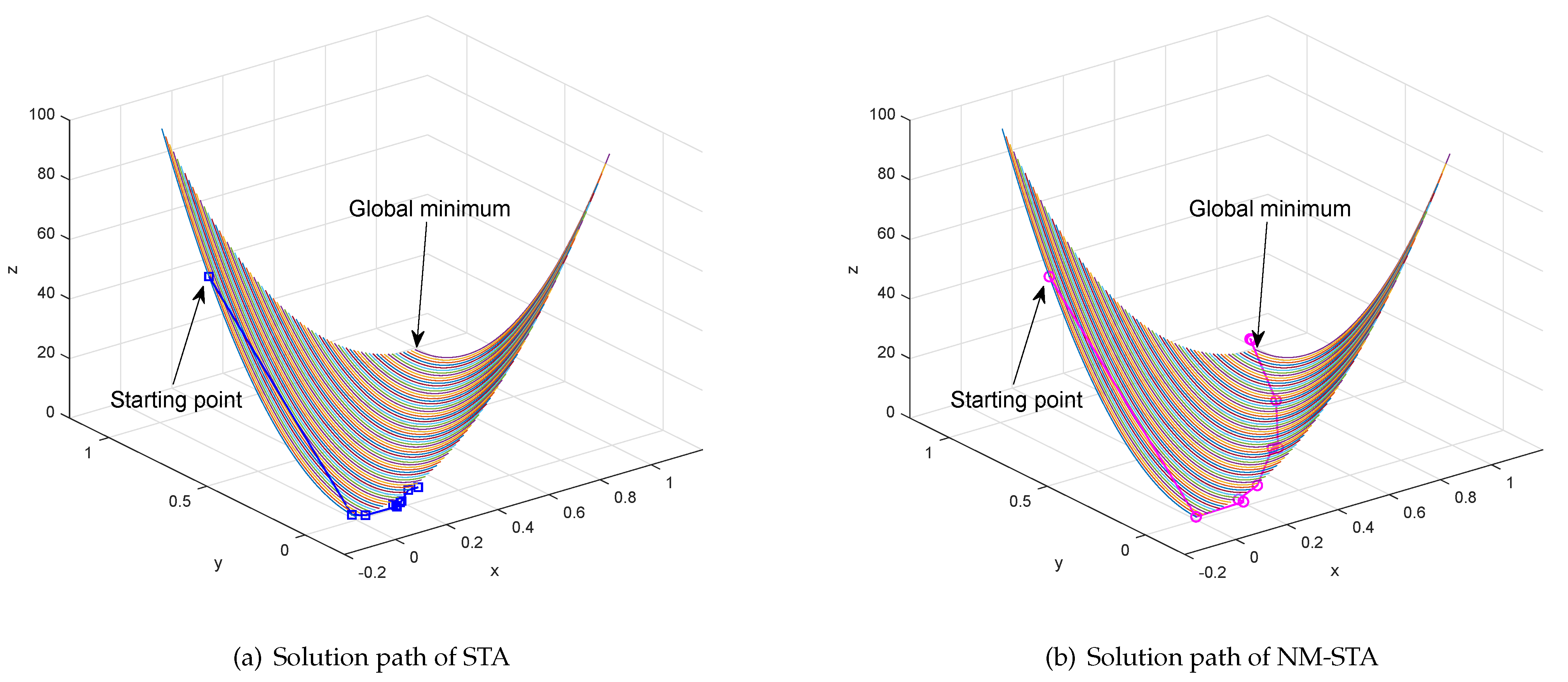
To demonstrate the faster convergence speed of NM-STA, a 2-D Rosenbrock test function is used. This unimodal function has a global minimum (1,1) that lies in a narrow, parabolic valley. The valley is easy to reach but further convergence is very difficult [44]. In the test for Rosenbrock function, the methods are terminated if the current solution x c u r r e n t satisfies:
f ( x c u r r e n t ) f ( B e s t ) ϵ
where B e s t indicates the global minimum. If the specified accuracy ϵ is met, the test is considered as a ‘success’. In this section, ϵ is set at 1 × 10 8 .
The statistical results given in Table 1 reveal that NM-STA is able to reach the same accuracy with much less FEs. In Figure 4, the solution paths of STA and NM-STA on the Rosenbrock function are portrayed, where both methods start from the same starting point (0, 0.75), and only the first 10 solutions are plotted in the figures for the convenience of observation. It is clear that the solution path of NM-STA is much more efficient.
By comparing the two paths, it can be seen that both methods quickly reach the valley. After that, STA searches aimlessly in the valley and moves slowly while NM-STA finds a promising direction and moves towards the optimum efficiently. This brief experiment demonstrates that the utilization of historical information can lead to a more promising search direction; therefore, NM-STA has a faster convergence speed than basic STA.

3.3. Combination NM-STA with QI

As discussed above, STA and NM simplex search are optimization methods with distinct characteristics. As a novel metaheuristic method, STA has a strong global exploration capacity; however, its convergence speed and exploitation capacity decrease in the later stages of searching. As a classical direct search method, NM simplex search has a fast convergence speed but is not stable in global search. However, when it comes to the neighbor of the global minimum, both STA and NM are not very powerful. On the contrary, QI is able to approximate the global minimum by an analytical solution but is only effective when the search agents are close enough to the global minimum. Thus, QI is used in the hybrid STA.
To invoke QI in later stage of the search, the average accuracy of the solutions in the historical information set H is calculated in each iteration as:
A A S = f x 1 + f x 2 + + f x D + 1 D + 1 f ( B e s t )
where B e s t indicates the global best solution.
If A A S meets a certain threshold value, the solutions are considered to be in the neighborhood of the global optimum. Then, QI will be invoked to improve the solution accuracy. In the implementation of QI, two QI search agents x a and x b are randomly chosen from the historical information set H , and the third search agent x b e s t is the current best solution.

3.4. The Hybrid STA (NMQI-STA)

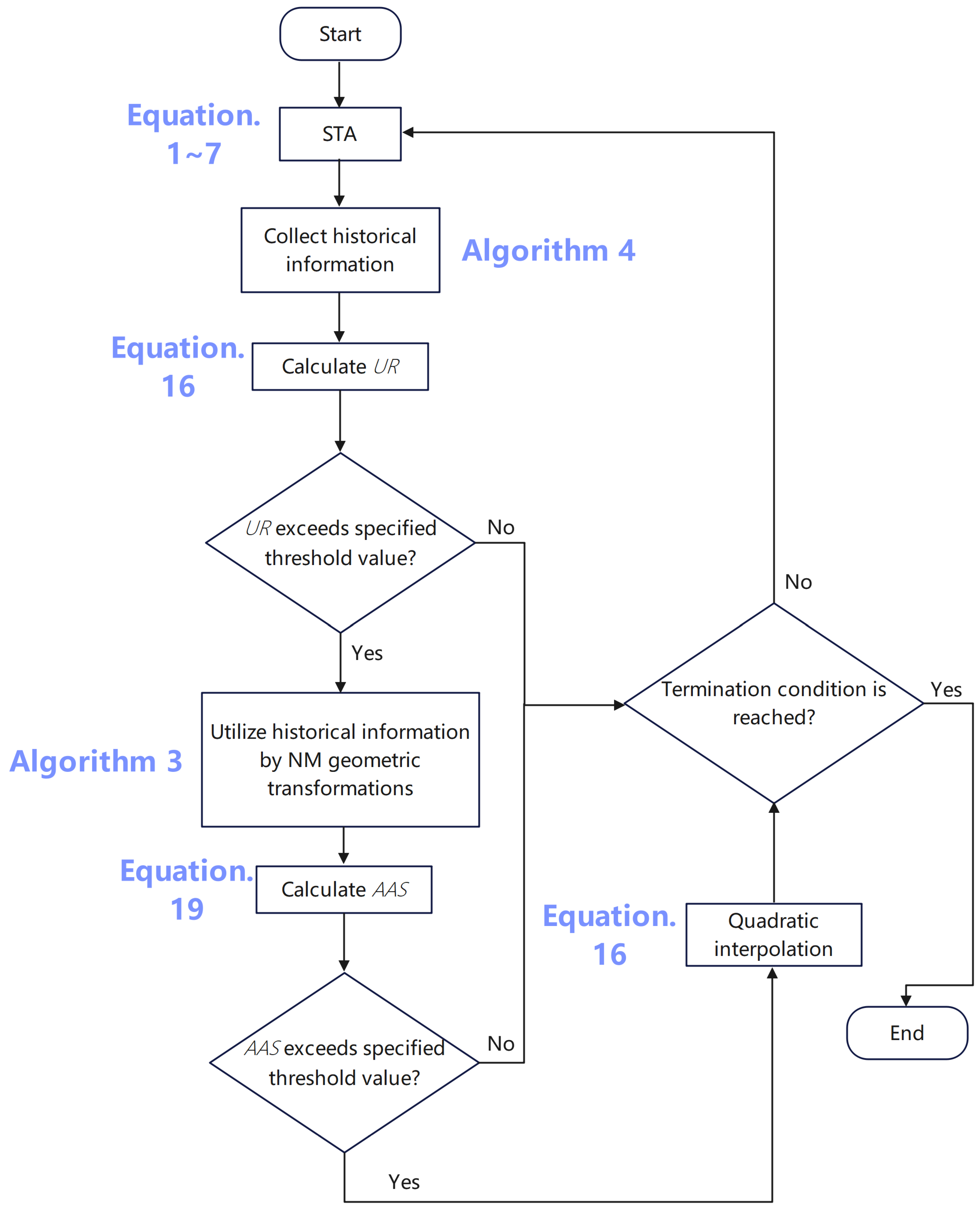
To combine the merits of the three methods, NM simplex search and QI are applied to utilize the historical information of STA. Therefore, an enhanced hybrid STA based on NM simplex search and QI (NMQI-STA) is proposed. The hybrid STA’s step-wise procedure is summarized as follows:
Step 1:
Produce solutions randomly as original solutions.
Step 2:
Use state transformation operators to produce current solutions. Every best solution found by the operators will be placed into the historical information set H.
Step 3:
Calculate the value of U R . If U R meets the threshold value, go to Step 4; otherwise, go back to Step 2.
Step 4:
Utilize the historical information in H based on NM geometric transformations to update H and the current best solution.
Step 5:
Calculate the value of A A S . If A A S meets the threshold value, go to Step 6; otherwise, go back to Step 2.
Step 6:
Utilize QI with the historical information in H.
Step 7:
Check whether the termination conditions are met. If not, go back to Step 2; otherwise, the algorithm is terminated.
As shown in Figure 5, the proposed method uses an eagle strategy [45] to maximize the efficiency and stability. In the exploration stage, NM simplex search utilizes the historical information of STA to generate promising solutions. As a result, the convergence speed is continuously accelerated. In the exploitation stage, QI utilizes the historical information to enhance the local search capacity. Consequently, the solution accuracy is improved.
For comparison, a hybrid STA with QI (QI-STA) was also implemented. The strategy of QI-STA is essentially the same as NMQI-STA. The only difference is that the NM simplex search is disabled in QI-STA.

4. Experimental Results and Discussions

We tested the proposed method against a set of benchmark functions. All methods were implemented in a MATLAB R2018a environment with an Intel Core i7-7700, 3.60 GHz processor on a 64-bit Windows 10 operating system.

4.1. Benchmark Functions and Parameter Settings

The details of the benchmark functions are shown in Table 2. Notably, f min and R a n g e indicate the global optimal value and the range of the search space. Generally, in Table 2, there are two types of benchmark functions, called unimodal and multimodal. A function with a single minimum in the specified range is called unimodal. Unlike unimodal, multimodal functions have many local minimums that the method may be trapped in.
All the parameter settings of other algorithms were the same as in the references. For all members in the STA family, S E was set to 50, T p was set to 10, the threshold value for U R was set to 0.5, and the threshold value for A A S was set to 1 × 10 6 . To guarantee fairness and avoid arbitrariness, each test in the following experiments was performed 30 times independently. In each independent test, a method was terminated if any of the following criteria were satisfied:
  • The global minimum of the objective function is found.
  • The maximum number of function evaluations is attained.

4.2. Comparison with Other Metaheuristic Methods

To examine the effectiveness of the hybrid STA, several population-based metaheuristic methods were used, including ABC [16,17], CLPSO [46,47], GWO [48,49], MVO [50,51], SSA [52,53] and WOA [54,55]. These meteheuristic methods have been applied in various fields and have achieved state-of-the-art performance in different problems. For each benchmark function, the number of decision variables D was set to 20, 30, 50 and 100, respectively. The computational results are listed in Table 3, Table 4, Table 5 and 
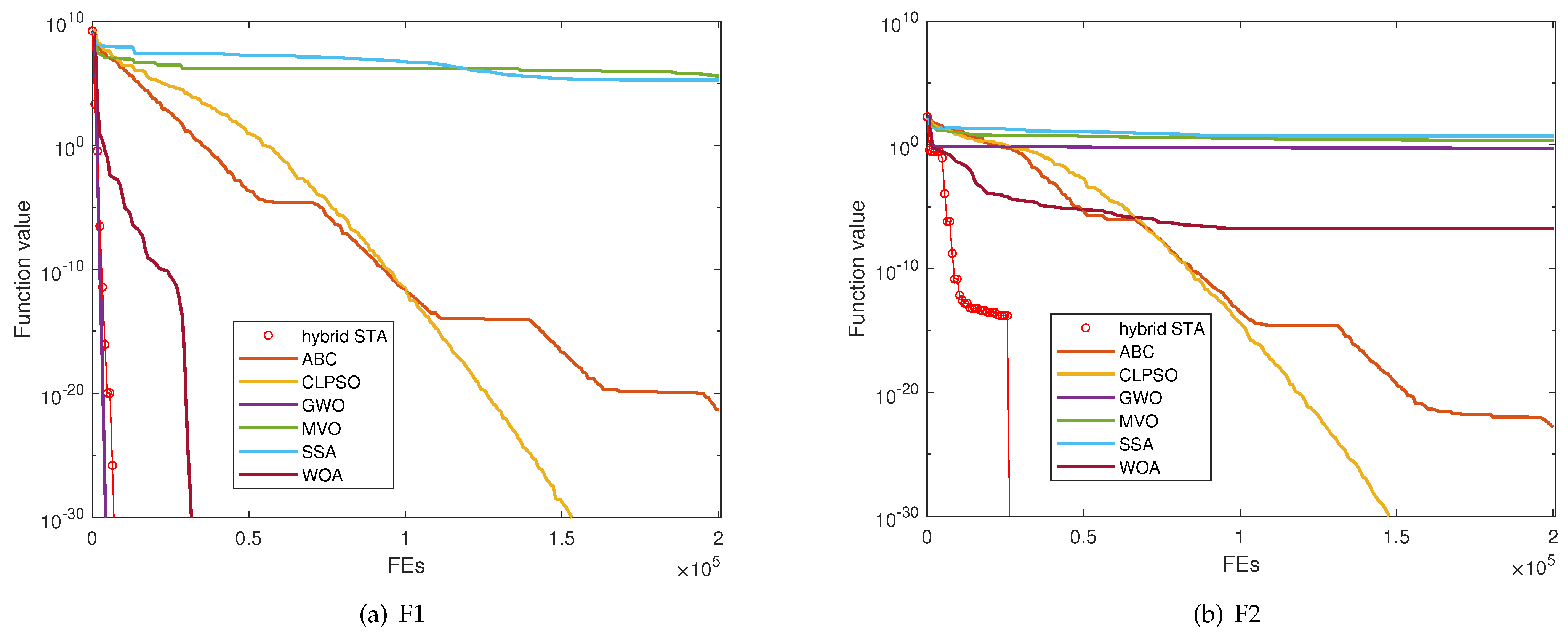
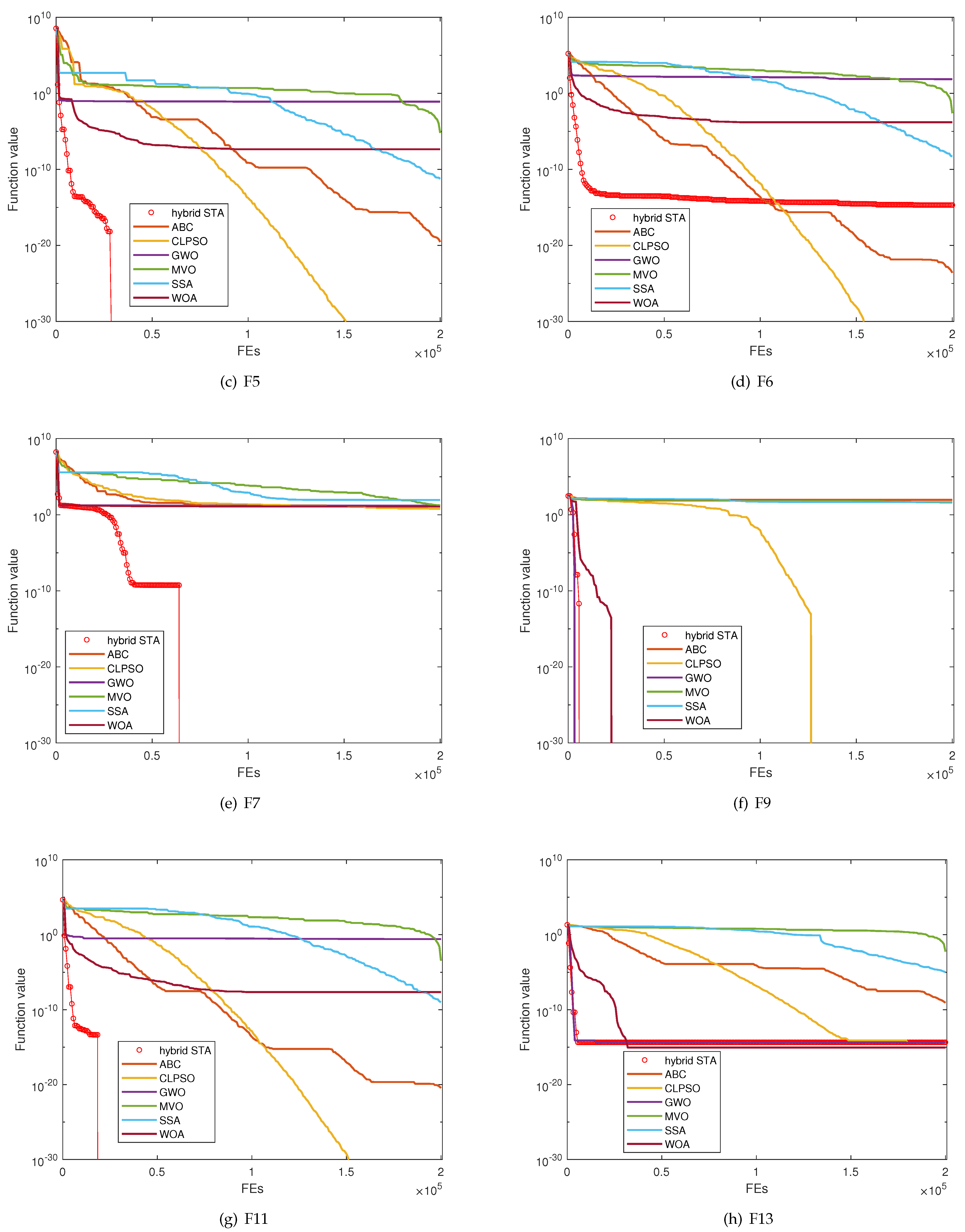
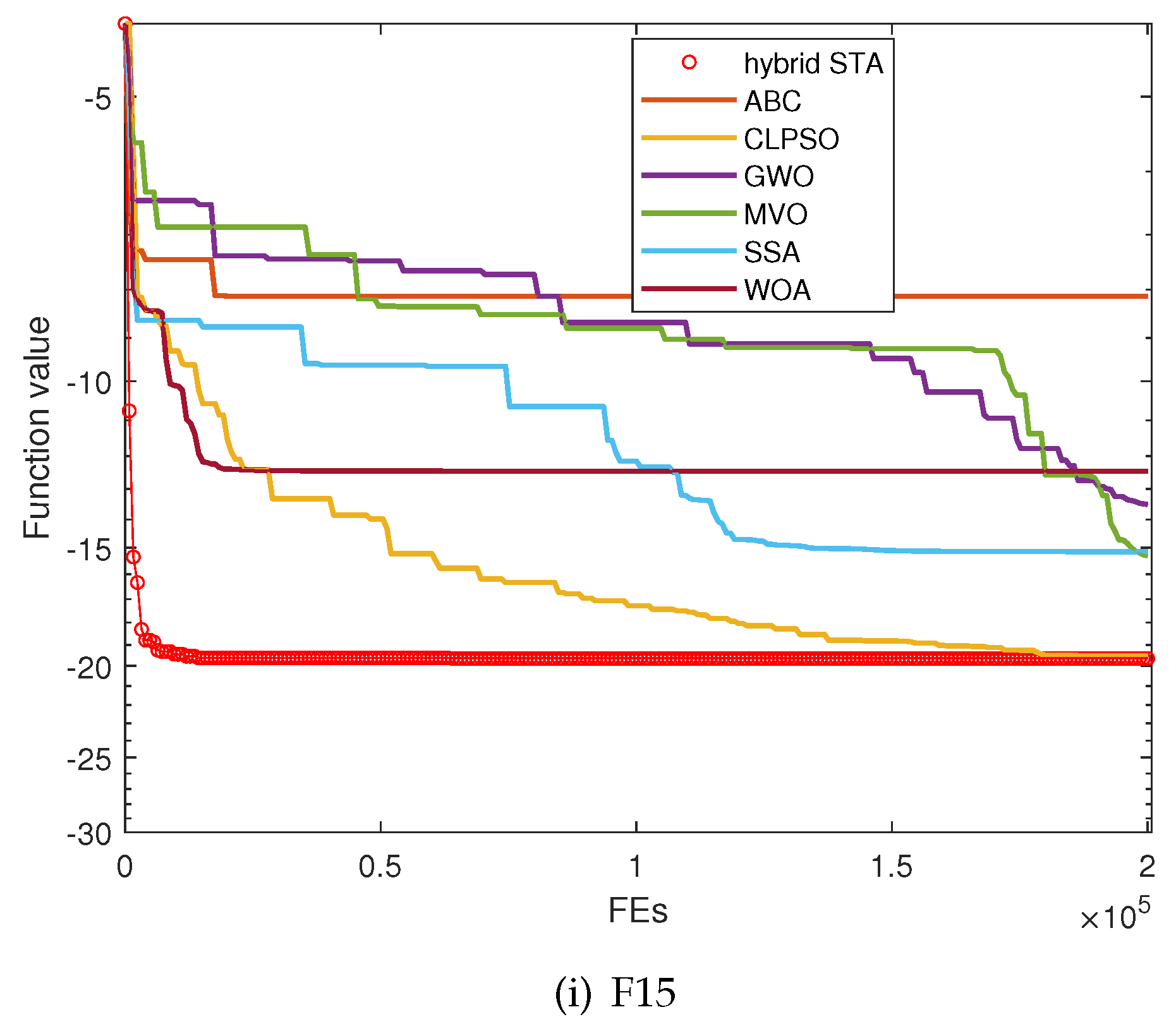
Table 6, and the average convergence curves of all test functions with D = 20 are given in Figure 6.
As shown in the experiment results, the hybrid STA outperformed ABC, CLPSO, GWO, MVO and SSA in most of the cases. Despite WOA demonstrating better performance on functions such as F3 and F13, the hybrid STA performed better than WOA in the other 10 benchmark functions. WOA failed to remain stable in finding acceptable solutions on F2, F7, F8, F11 and F14. On the contrary, the hybrid STA showed incomparably convergence speed and solution accuracy on F8 and 11 and showed more robustness on multimodal functions, such as F2, F7 and F14. Therefore, the proposed method was more effective and robust than these competitive metaheuristic methods.

4.3. Comparison among the STA Family

To comprehensively verify the effect of NM simplex search and QI in the proposed method, the STA family (STA, NM-STA, QI-STA and hybrid STA) were tested against the benchmark functions listed in Table 2. For each benchmark function, the number of decision variables 
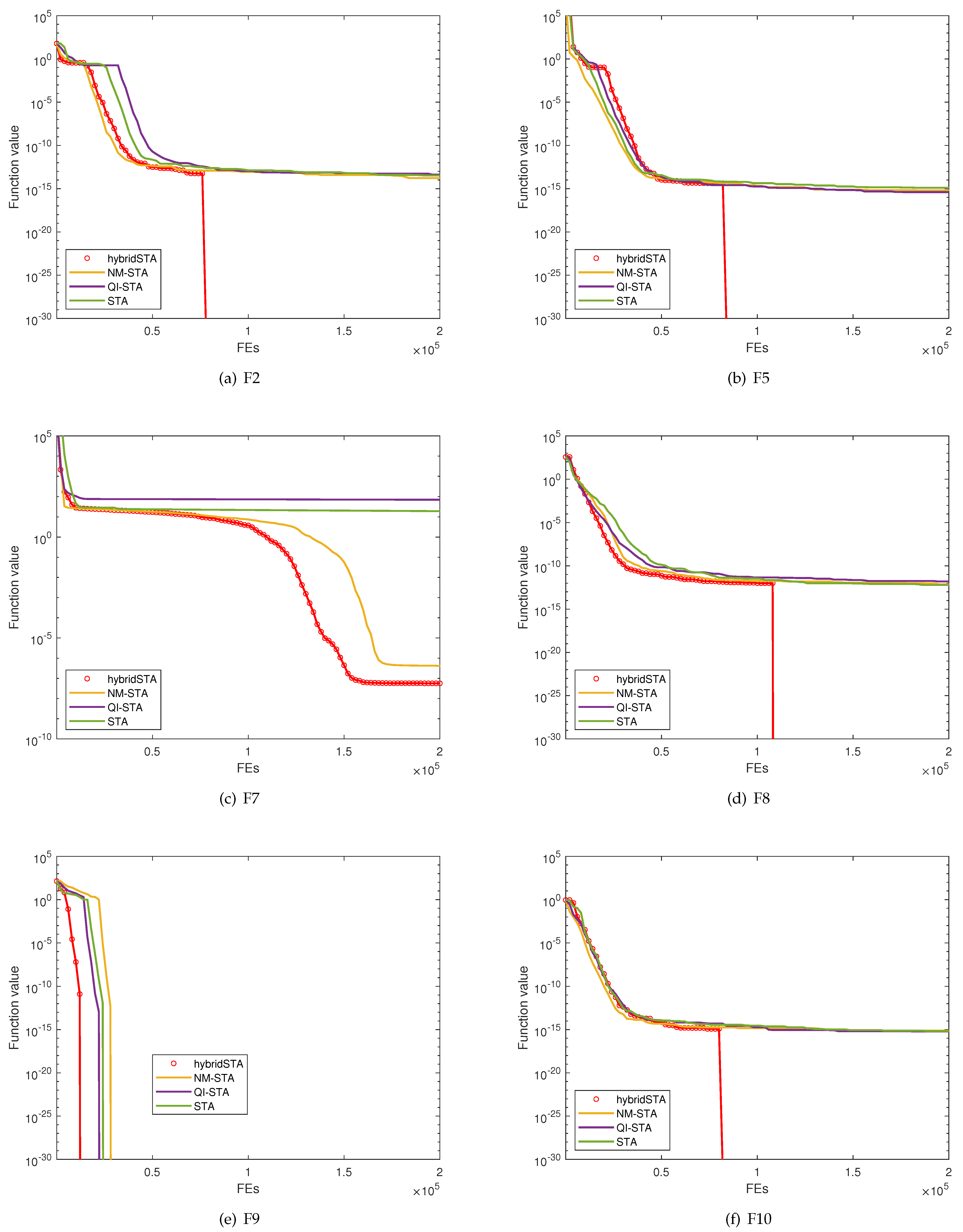
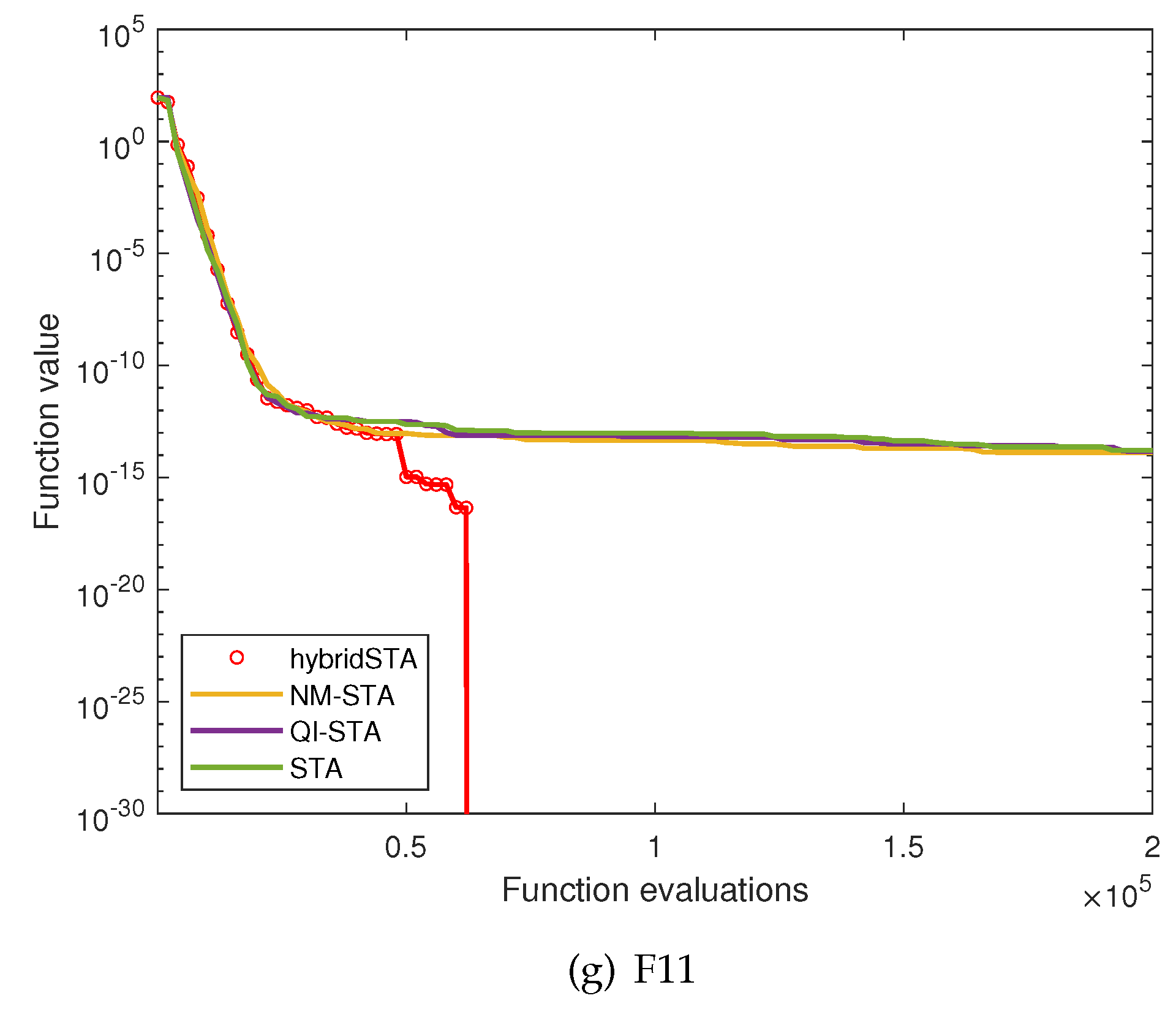
D was set to 30. The statistical results are shown in Table 7, and the average convergence curves are given in Figure 7.
As shown in the experiment results, both the convergence speed and accuracy of the hybrid STA were better than for STA. The average FEs of the hybrid STA were much less than those for STA on F1, F8, F9 and F11, which means that the convergence speed of the hybrid STA was much faster than STA. The convergence accuracy of STA was significantly improved on F1, F2, F5, F7, F8 and F10.
From the above discussion, when STA is enhanced with both NM simplex search and QI, the merits of the three distinct methods are combined. The convergence curves and the statistical results show that hybrid STA combines the merits of all three: the powerful exploration capacity of STA, the fast convergence speed of NM simplex search and the deep exploitation capacity of QI.

4.4. Effectiveness Analysis

In order to evaluate the effectiveness of hybrid STA, the overall effectiveness ( O E ) [56], which is a useful metric, is computed in this section. The OE of each algorithm is calculated using Equation (20), where N presents the number of test functions and L presents the losing test functions of each algorithm. The results are reported in Table 8.
O E i ( % ) = 1 L i N

4.5. Non-Parametric Statistical Test Analysis

In Table 3, Table 4, Table 5 and Table 6, the first results of these algorithms’ performances are presented. To compare the effectiveness of hybrid STA statistically, a powerful and sensitive non-parametric test, named the Wilcoxon signed-rank sum test, is performed. This test, where the p-value is computed with a statistical significance value α = 0.05, can present the significant difference between pairs of algorithms. The results of the test for dimensions of 20, 30, 50 and 100 are listed in Table 9, Table 10, Table 11 and Table 12. The results of p-value < α indicate that the hybrid STA had better performance than the compared algorithms.

5. Wireless Sensor Network Application

A wireless sensor network (WSN) is a self-organizing network composed of a large number of sensor nodes deployed in a predetermined area [57]. A WSN can monitor the information in the deployment area and deliver effective information in the real time. The node-positioning technology of sensor is the basis of the entire wireless sensor network. As it is widely used in medical, military, environmental science, space exploration and other fields, the requirements on its positioning accuracy are continually increasing [58,59,60,61,62].
Many researchers have applied the metaheuristic method with a node-positioning algorithm. Wang [63] proposed a PSO clustering algorithm based on mobile aggregation for WSN. The algorithm used PSO to perform virtual clustering in the routing process, which improved the positioning accuracy and reduced the transmission delay. Sharma [64] proposed a genetic algorithm based on the improved distance vector Hop and applied it to the WSN positioning problem to improve the positioning accuracy. Cui [65] obtained the estimated location of unknown nodes using a differential evolution algorithm, which effectively reduced the range error and obtained high positioning accuracy.

5.1. Wireless Sensor Network Localization Problem

There are m anchor nodes a 1 , a 2 , , a m R d (d represents the dimensions, which are two or three), and there are n unknown nodes x 1 , x 2 , , x n R d . The Euclidean distance between the i t h unknown node and j t h unknown node is called d i j , and ( i , j ) N x . The Euclidean distance between the i t h unknown node and k t h anchor node is called d ¯ i k , and ( i , k ) N a . Furthermore, N x = { ( i , j ) : x i x j = d i j r d } , and N a = { ( i , k ) : x i a k = d ¯ i k r d } , where r d represents the sensor communication distance.
The wireless sensor network localization problem (SNL) is to estimate the position of n unknown nodes x i ( i = 1 , , n ) , which should satisfy:
x i x j 2 = d i j 2 , ( i , j ) N x ,
x i a k 2 = d ¯ i k 2 , ( i , k ) N a .
Considering that there is noise in the real situation, there is no guarantee that the formula above is workable. To make the model universal, the SNL is reformulated as the following non-convex optimization problem by using the least-squares algorithm:
min ( i , j ) N x ( x i x j 2 d i j 2 ) 2 + ( i , k ) N a ( x i a k 2 d ¯ i k 2 ) 2 .

5.2. Experimental Results and Analysis

To further test the performance of hybrid STA, it was applied to the SNL problem. Furthermore, it was compared with other optimization algorithms, such as ABC, CLPSO, GWO, WOA, MVO and SSA. All the parameter settings of other algorithms were the same as in the references.
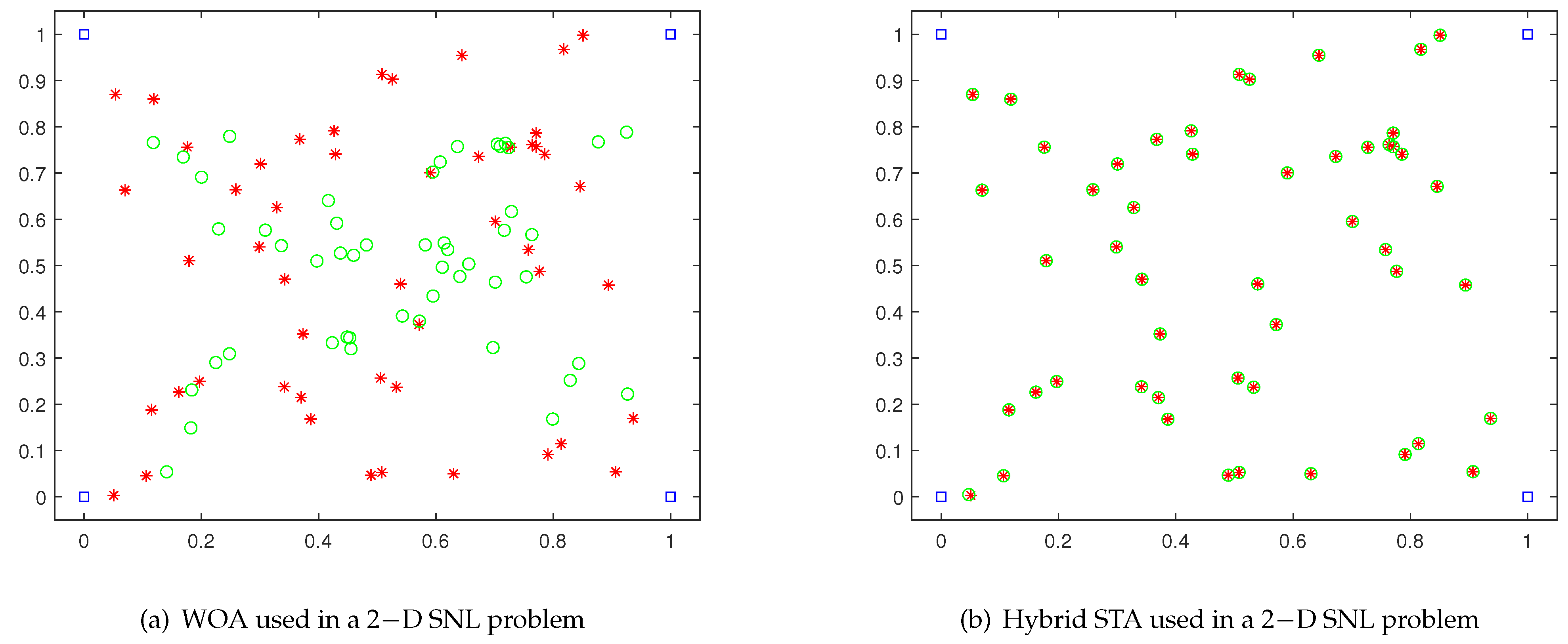
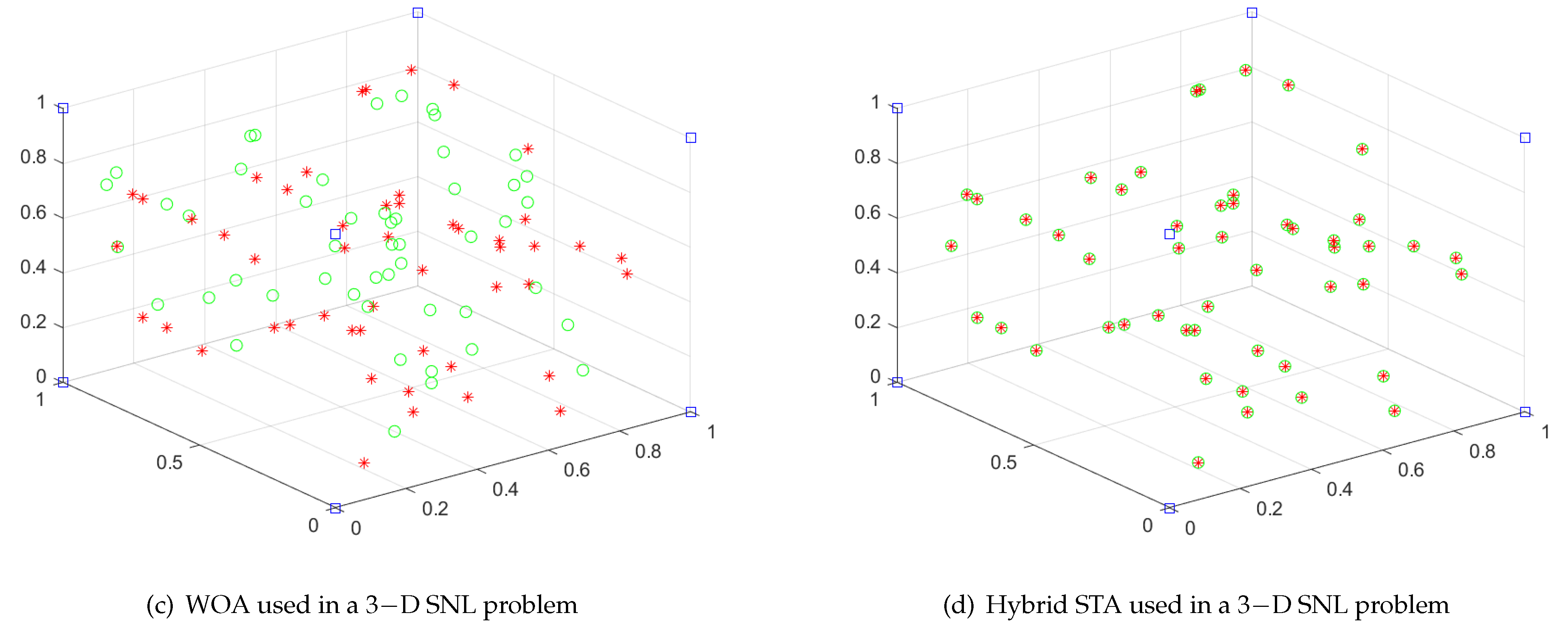
In the two-dimensional SNL problem, the number of anchor nodes was set as 4, and the number of unknown nodes was set as 50. The coordinates of the anchor nodes were (0,0), (0,1), (1,0) and (1,1). The radio range was 0.3. In the three-dimensional SNL problem, the number of anchor nodes was set as 8, and the number of unknown nodes was set as 50. The coordinates of the anchor nodes were (0,0,0), (0,0,1), (0,1,0), (1,0,0), (1,1,0), (1,0,1), (0,1,1) and (1,1,1). The radio range was 0.35. In Figure 8, the data marked in red are the true locations of the unknown nodes, and the data marked in green are the locations of the nodes as calculated by the algorithms. Furthermore, the data marked in blue are the locations of the anchor nodes.
Figure 8a,b show the localization results of the WOA in two-dimensional and three- dimensional SNL problems. Figure 8c,d show the localization results of the hybrid STA in the two-dimensional and three-dimensional SNL problems. After using the hybrid STA, the estimation location almost coincided with the true location. However, after using the WOA, the estimation error remained large between the estimation location and the true location. In the SNL problem, the hybrid STA performed much better than WOA. 
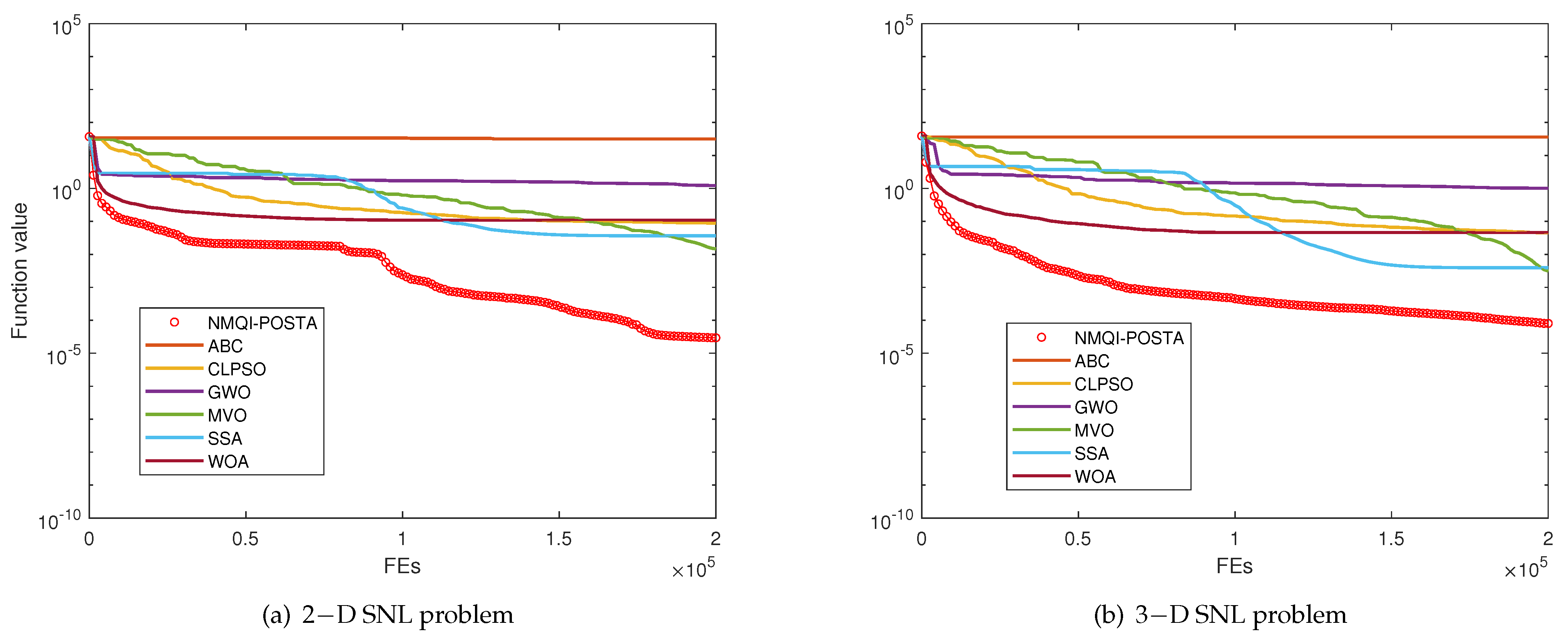
Figure 9a,b show the convergent curves of the hybrid STA and other methods for the 2-D and 3-D SNL problems, respectively. Compared with other metaheuristic methods, the optimization accuracy and convergence speed of the hybrid STA were clearly better compared with the other algorithms.

6. Conclusions

In this paper, we proposed a hybrid STA based on Nelder–Mead simplex search and QI. In the hybrid STA, both NM simplex search and QI were applied to utilize the historical information. Specifically, in the exploration stage, NM simplex search utilized the historical information of STA to generate promising solutions. In the exploitation stage, QI utilized the historical information to enhance the local search capacity.
The proposed method used an eagle strategy to maximize the efficiency and stability. The proposed method enjoys the merits of the three methods: the global exploration capacity of STA, the fast convergence speed of NM simplex search and the strong exploitation ability of QI. The superiority and effectiveness of the proposed method was demonstrated by testing on 15 benchmark functions as well as the SNL problem and was compared with six other well-known metaheuristic methods.
In the proposed hybrid method, an eagle strategy was used to control the selection of vertices in the NM stage. However, the selection of vertices requires further study. In our future work, the quantitative properties of the vertices will be considered in the collection of historical information. It would also be interesting to apply the proposed historical information mechanism to other metaheuristic methods. In addition, other approaches of utilizing the historical information will be considered as well.

Author Contributions

Conceptualization, X.Z.; Methodology, L.Z. and X.Z.; Software, L.Z. and C.Y.; Validation, L.Z.; Writing–original draft, L.Z. and C.Y.; Writing–review & editing, X.Z. and C.Y.; Supervision, X.Z.; Funding acquisition, X.Z. All authors have read and agreed to the published version of the manuscript.

Funding

This research was funded by the National Natural Science Foundation of China under Grant 62273357 and the Hunan Provincial Natural Science Foundation of China under Grant 2021JJ20082.

Data Availability Statement

Due to privacy or ethical restrictions, data is unavailable.

Conflicts of Interest

The authors declare no conflict of interest.

References

  1. Kvasov, D.E.; Mukhametzhanov, M.S. Metaheuristic vs. deterministic global optimization algorithms: The univariate case. Appl. Math. Comput. 2018, 318, 245–259. [Google Scholar] [CrossRef]
  2. Dokeroglu, T.; Sevinc, E.; Kucukyilmaz, T.; Cosar, A. A survey on new generation metaheuristic algorithms. Comput. Ind. Eng. 2019, 137, 106040. [Google Scholar] [CrossRef]
  3. Whitley, D. A genetic algorithm tutorial. Stat. Comput. 1994, 4, 65–85. [Google Scholar] [CrossRef]
  4. Storn, R.; Price, K. Differential evolution—A simple and efficient heuristic for global optimization over continuous spaces. J. Glob. Optim. 1997, 11, 341–359. [Google Scholar] [CrossRef]
  5. Zamani, H.; Nadimi-Shahraki, M.H.; Gandomi, A.H. QANA: Quantum-based avian navigation optimizer algorithm. Eng. Appl. Artif. Intell. 2021, 104, 104314. [Google Scholar] [CrossRef]
  6. Nadimi-Shahraki, M.H.; Zamani, H. DMDE: Diversity-maintained multi-trial vector differential evolution algorithm for non-decomposition large-scale global optimization. Expert Syst. Appl. 2022, 198, 116895. [Google Scholar] [CrossRef]
  7. Russell, E.; James, K. A new optimizer using particle swarm theory. In Proceedings of the Sixth International Symposium on Micro Machine and Human Science, MHS’95, Nagoya, Japan, 4–6 October 1995; pp. 39–43. [Google Scholar]
  8. Wang, H.; Liang, M.N.; Sun, C.L.; Zhang, G.C.; Xie, L.P. Multiple-strategy learning particle swarm optimization for large-scale optimization problems. Complex Intell. Syst. 2021, 7, 1–16. [Google Scholar] [CrossRef]
  9. Li, W.; Zhang, L.; Chen, X.; Wu, C.; Cui, Z.; Niu, C. Predicting the evolution of sheet metal surface scratching by the technique of artificial intelligence. Int. J. Adv. Manuf. Technol. 2021, 112, 853–865. [Google Scholar] [CrossRef]
  10. Shami, T.M.; El-Saleh, A.A.; Alswaitti, M.; Al-Tashi, Q.; Summakieh, M.A.; Mirjalili, S. Particle swarm optimization: A comprehensive survey. IEEE Access 2022, 10, 10031–10061. [Google Scholar] [CrossRef]
  11. van Laarhoven, P.J.M.; Aarts, E.H.L. Simulated annealing. Stat. Sci. 1993, 8, 10–15. [Google Scholar]
  12. Rashedi, E.; Nezamabadi-Pour, H.; Saryazdi, S. GSA: A gravitational search algorithm. Inf. Sci. 2009, 179, 2232–2248. [Google Scholar] [CrossRef]
  13. Sajwan, A.; Yadav, A. AEFA: Artificial electric field algorithm for global optimization. Swarm Evol. Comput. 2019, 48, 93–108. [Google Scholar]
  14. Zhou, X.J.; Yang, C.H.; Gui, W.H. State transition algorithm. J. Ind. Manag. Optim. 2012, 8, 1039. [Google Scholar] [CrossRef] [Green Version]
  15. Zhou, X.J.; Yang, C.H.; Gui, W.H. The principle of state transition algorithm and its applications. Acta Autom. Sin. 2020, 46, 2260–2274. [Google Scholar]
  16. Karaboga, D.; Basturk, B. A powerful and efficient algorithm for numerical function optimization: Artificial bee colony (abc) algorithm. J. Glob. Optim. 2007, 39, 459–471. [Google Scholar] [CrossRef]
  17. Ebubekir, K.; Beyza, G.; Bahriye, A.; Dervis, K. A review on the studies employing artificial bee colony algorithm to solve combinatorial optimization problems. Eng. Appl. Artif. Intell. 2022, 115, 105311. [Google Scholar]
  18. Zhang, F.X.; Yang, C.H.; Zhou, X.J. Fractional order fuzzy PID optimal control in copper removal process of zinc hydrometallurgy. Hydrometallurgy 2018, 178, 60–76. [Google Scholar] [CrossRef]
  19. Zhang, F.X.; Yang, C.H.; Zhou, X.J. Optimal setting and control strategy for industrial process based on discrete-time fractional-order (PID mu)-D-lambda. IEEE Access 2019, 7, 47747–47761. [Google Scholar] [CrossRef]
  20. Han, J.; Yang, C.H.; Zhou, X.J.; Gui, W.H. A new multi-threshold image segmentation approach using state transition algorithm. Appl. Math. Model. 2017, 44, 588–601. [Google Scholar] [CrossRef]
  21. Zhou, X.J.; Yang, C.H.; Gui, W.H. Nonlinear system identification and control using state transition algorithm. Appl. Math. Comput. 2014, 226, 169–179. [Google Scholar] [CrossRef] [Green Version]
  22. Huang, Z.K.; Yang, C.H.; Zhou, X.J.; Huang, T.W. A hybrid feature selection method based on binary state transition algorithm and ReliefF. IEEE J. Biomed. Health Inform. 2018, 23, 1888–1898. [Google Scholar] [CrossRef] [PubMed]
  23. Wang, Q.; Huang, M.; Zhou, X.J. Feature selection in froth flotation for production condition recognition. IFAC-PapersOnLine 2018, 51, 123–128. [Google Scholar] [CrossRef]
  24. Wang, C.; Zhang, H.L.; Ma, P. Wind power forecasting based on singular spectrum analysis and a new hybrid Laguerre neural network. Appl. Energy 2020, 259, 114139. [Google Scholar] [CrossRef]
  25. Dong, Y.C.; Zhang, H.L.; Wang, C.; Zhou, X.J. Wind power forecasting based on stacking ensemble model, decomposition and intelligent optimization algorithm. Neurocomputing 2021, 462, 169–184. [Google Scholar] [CrossRef]
  26. Zhou, X.; Sun, Y.; Huang, Z.; Yang, C.; Yen, G.G. Dynamic multi-objective optimization and fuzzy AHP for copper removal process of zinc hydrometallurgy. Appl. Soft Comput. 2022, 129, 109613. [Google Scholar] [CrossRef]
  27. Lin, F.; Zhou, X.; Li, C.; Huang, T.; Yang, C. Data-driven state transition algorithm for fuzzy chance-constrained dynamic optimization. IEEE Trans. Neural Netw. Learn. Syst. 2022, 71, 102937. [Google Scholar] [CrossRef]
  28. Wang, Z.Y.; Zhou, X.J.; Tian, J.T.; Huang, T.W. Hierarchical parameter optimization based support vector regression for power load forecasting. Sustain. Cities Soc. 2021, 71, 102937. [Google Scholar] [CrossRef]
  29. Zhou, X.J.; Huang, M.; Huang, T.W.; Yang, C.H.; Gui, W.H. Dynamic optimization for copper removal process with continuous production constraints. IEEE Trans. Ind. Inform. 2019, 16, 7255–7263. [Google Scholar] [CrossRef]
  30. Zhou, X.; Yang, C.; Gui, W. A statistical study on parameter selection of operators in continuous state transition algorithm. IEEE Trans. Cybern. 2018, 49, 3722–3730. [Google Scholar] [CrossRef] [Green Version]
  31. Nelder, J.A.; Mead, R. A simplex method for function minimization. Comput. J. 1965, 7, 308–313. [Google Scholar] [CrossRef]
  32. Yalçınkaya, A.; Şenoğlu, B.; Yolcu, U. Maximum likelihood estimation for the parameters of skew normal distribution using genetic algorithm. Swarm Evol. Comput. 2018, 38, 127–138. [Google Scholar] [CrossRef]
  33. Wu, G.; Mallipeddi, R.; Suganthan, P. Ensemble strategies for population-based optimization algorithms—A survey. Swarm Evol. Comput. 2019, 44, 695–711. [Google Scholar] [CrossRef]
  34. Cruz-Duarte, J.M.; Amaya, I.; Ortiz-Bayliss, J.C.; Conant-Pablos, S.E.; Terashima-Marín, H.; Shi, Y. Hyper-heuristics to customise metaheuristics for continuous optimization. Swarm Evol. 2021, 100935. [Google Scholar] [CrossRef]
  35. Chen, X.; Mei, C.; Xu, B.; Yu, K.; Huang, X. Quadratic interpolation based teaching-learning-based optimization for chemical dynamic system optimization. Knowl.-Based Syst. 2018, 145, 250–263. [Google Scholar] [CrossRef]
  36. Sun, Y.; Yang, T.; Liu, Z. A whale optimization algorithm based on quadratic interpolation for high-dimensional global optimization problems. Appl. Soft Comput. 2019, 85, 105744. [Google Scholar] [CrossRef]
  37. Guo, W.; Wang, Y.; Dai, F.; Xu, P. Improved sine cosine algorithm combined with optimal neighborhood and quadratic interpolation strategy. Eng. Appl. Artif. Intell. 2020, 94, 103779. [Google Scholar] [CrossRef]
  38. Skanderova, L.; Fabian, T.; Zelinka, I. Self-organizing migrating algorithm using covariance matrix adaptation evolution strategy for dynamic constrained optimization. Swarm Evol. Comput. 2021, 65, 100936. [Google Scholar] [CrossRef]
  39. Gao, F.; Han, L. Implementing the nelder-mead simplex algorithm with adaptive parameters. Comput. Optim. Appl. 2012, 51, 259–277. [Google Scholar] [CrossRef]
  40. Yang, Y.; Zong, X.; Yao, D.; Li, S. Improved alopex-based evolutionary algorithm (aea) by quadratic interpolation and its application to kinetic parameter estimations. Appl. Soft Comput. 2017, 51, 23–38. [Google Scholar] [CrossRef]
  41. Kang, F.; Li, J.; Xu, Q. Structural inverse analysis by hybrid simplex artificial bee colony algorithms. Comput. Struct. 2009, 87, 861–870. [Google Scholar] [CrossRef]
  42. Yildiz, A.R. A novel hybrid whale–nelder–mead algorithm for optimization of design and manufacturing problems. Int. J. Adv. Manuf. Technol. 2019, 105, 5091–5104. [Google Scholar] [CrossRef]
  43. Xu, S.; Wang, Y.; Wang, Z. Parameter estimation of proton exchange membrane fuel cells using eagle strategy based on jaya algorithm and nelder-mead simplex method. Energy 2019, 173, 457–467. [Google Scholar] [CrossRef]
  44. Picheny, V.; Wagner, T.; Ginsbourger, D. A benchmark of kriging-based infill criteria for noisy optimization. Struct. Multidiscip. Optim. 2013, 48, 607–626. [Google Scholar] [CrossRef] [Green Version]
  45. Yang, X.-S.; Deb, S. Two-stage eagle strategy with differential evolution. Int. J.-Bio-Inspired Comput. 2012, 4, 1–5. [Google Scholar] [CrossRef] [Green Version]
  46. Liang, J.J.; Qin, A.K.; Suganthan, P.N.; Baskar, S. Comprehensive learning particle swarm optimizer for global optimization of multimodal functions. IEEE Trans. Evol. Comput. 2006, 10, 281–295. [Google Scholar] [CrossRef]
  47. Zhang, X.; Sun, W.; Xue, M.; Lin, A. Probability-optimal leader comprehensive learning particle swarm optimization with Bayesian iteration. Appl. Soft Comput. 2021, 103, 107132. [Google Scholar] [CrossRef]
  48. Mirjalili, S.; Mirjalili, S.M.; Lewis, A. Grey wolf optimizer. Adv. Eng. Softw. 2014, 69, 46–61. [Google Scholar] [CrossRef] [Green Version]
  49. Makhadmeh, S.N.; Khader, A.T.; Al-Betar, M.A.; Naim, S.; Abasi, A.K.; Alyasseri, Z.A.A. A novel hybrid grey wolf optimizer with min-conflict algorithm for power scheduling problem in a smart home. Swarm Evol. Comput. 2021, 60, 100793. [Google Scholar] [CrossRef]
  50. Mirjalili, S.; Mirjalili, S.M.; Hatamlou, A. Multi-verse optimizer: A nature-inspired algorithm for global optimization. Neural Comput. Appl. 2016, 27, 495–513. [Google Scholar] [CrossRef]
  51. Abualigah, L.; Alkhrabsheh, M. Amended hybrid multi-verse optimizer with genetic algorithm for solving task scheduling problem in cloud computing. Neural Comput. Appl. 2022, 78, 740–765. [Google Scholar] [CrossRef]
  52. Xue, J.K.; Shen, B. A novel swarm intelligence optimization approach: Sparrow search algorithm. Syst. Sci. Control. Eng. 2020, 8, 22–34. [Google Scholar] [CrossRef]
  53. Gao, B.W.; Shen, W.; Guan, H.; Zheng, L.T.; Zhang, W. Research on multistrategy improved evolutionary sparrow search algorithm and its application. IEEE Access 2022, 10, 62520–62534. [Google Scholar] [CrossRef]
  54. Mirjalili, S.; Lewis, A. The whale optimization algorithm. Adv. Eng. Softw. 2016, 95, 51–67. [Google Scholar] [CrossRef]
  55. Chakraborty, S.; Saha, A.K.; Sharma, S.; Mirjalili, S.; Chakraborty, R. A novel enhanced whale optimization algorithm for global optimization. Comput. Ind. Eng. 2021, 153, 107086. [Google Scholar] [CrossRef]
  56. Nadimi-Shahraki, M.H.; Taghian, S.; Mirjalili, S.; Faris, H. MTDE: An effective multi-trial vector-based differential evolution algorithm and its applications for engineering design problems. Appl. Soft Comput. 2020, 97, 106761. [Google Scholar] [CrossRef]
  57. Khurana, K.; Goyal, N. A survey on deployment strategies and energy efficiency of wireless sensor networks. Int. J. Electr. Electron. Comput. Sci. Eng. 2016, 3, 16–20. [Google Scholar]
  58. Elhoseny, M.; Farouk, A.; Zhou, N.R.; Wang, M.M.; Abdalla, S.; Batle, J. Dynamic multi-hop clustering in a wireless sensor network: Performance improvement. Wirel. Pers. Commun. 2017, 95, 3733–3753. [Google Scholar] [CrossRef]
  59. Juan, C.R.; Pablo, R.P.; Ernesto, S.; Rafael, G.L. A recursive shortest path routing algorithm with application for wireless sensor network localization. IEEE Sens. J. 2016, 16, 4631–4637. [Google Scholar]
  60. Zheng, J.Y.; Sun, Y.; Huang, Y.; Wang, Y.M.; Xiao, Y. Error analysis of range–based localisation algorithms in wireless sensor networks. Int. J. Sens. Netw. 2012, 12, 78–88. [Google Scholar] [CrossRef]
  61. Goyal, K.N.; Nain, M.; Singh, A.; Abualsaud, K.; Alsubhi, K.; Ortega-Mansilla, A.; Zorba, N. An Anchor-Based Localization in Underwater Wireless Sensor Networks for Industrial Oil Pipeline Monitoring. IEEE Can. J. Electr. Comput. Eng. 2022, 45, 466–474. [Google Scholar] [CrossRef]
  62. Goyal, K.N. An optimal scheme for minimizing energy consumption in WSN. Glob. Res. Dev. J. Eng. 2016, 1, 1–7. [Google Scholar]
  63. Wang, J.; Cao, Y.Q.; Li, B.; Kim, H.J.; Lee, S. Particle swarm optimization based clustering algorithm with mobile sink for WSNs. Future Gener. Comput. Syst. 2017, 76, 452–457. [Google Scholar] [CrossRef]
  64. Sharma, G.; Kumar, A. Improved range-free localization for three-dimensional wireless sensor networks using genetic algorithm. Comput. Electr. Eng. 2018, 72, 808–827. [Google Scholar] [CrossRef]
  65. Cui, L.Z.; Xu, C.; Li, G.H.; Ming, Z.; Feng, Y.H.; Lu, N. A high accurate localization algorithm with DV-Hop and differential evolution for wireless sensor network. Appl. Soft Comput. 2018, 68, 39–52. [Google Scholar] [CrossRef]
Figure 1. The geometric transformations in an NM simplex search.
Electronics 12 00994 g001
Figure 2. Comparison in utilizing history information.
Electronics 12 00994 g002
Figure 3. Comparison in collecting and utilizing historical information.
Electronics 12 00994 g003
Figure 4. Solution paths of STA and NM-STA on a Rosenbrock function.
Electronics 12 00994 g004
Figure 5. Flowchart of the enhanced hybrid STA.
Electronics 12 00994 g005
Figure 6. Average convergence curves of different metaheuristic methods on benchmark functions with D = 20.
Electronics 12 00994 g006aElectronics 12 00994 g006bElectronics 12 00994 g006c
Figure 7. Average convergence curves of the STA family on benchmark functions with D = 30.
Electronics 12 00994 g007aElectronics 12 00994 g007b
Figure 8. Optimization results of hybrid STA and WOA in 2–D and 3–D SNL problems.
Electronics 12 00994 g008aElectronics 12 00994 g008b
Figure 9. Average convergence curves of different metaheuristic methods in the SNL problems.
Electronics 12 00994 g009
Table 1. Statistical results for STA and NM-STA with D = 2.
FunctionSTANM-STA
Ave FEsSuccess RateAve FEsSuccess Rate
F7 1.08 × 10 4 30/30 4.54 × 10 3 30/30
Table 2. Benchmark function set.
Funtion NameEquationRange f min Modality
Elliptic F 1 = i = 2 D 10 6 ( i 1 ) / ( D 1 ) · x i 2 [ 100 , 100 ] 0Unimodal
Levy F 2 = sin 2 ( π w 1 ) + i = 1 D 1 ( w i 1 ) 2 ( 1 + 10 sin 2 ( π w i + 1 ) ) + ( w D 1 ) 2 ( 1 + sin 2 ( 2 π w D ) ) , w i = 1 + x i 1 4 [ 10 , 10 ] 0Multimodal
Levy and Montalvo 2 F 3 = 0.1 i = 1 D 1 x i 1 2 ( 1 + ( sin 2 ( 3 π x i + 1 ) ) ) + ( x D 1 ) 2 ( 1 + ( sin 2 ( 2 π x D ) ) ) + ( sin 2 ( 3 π x 1 ) ) [ 5 , 5 ] 0Multimodal
Pathological F 4 = i = 1 D 1 0.5 + sin 2 100 x i 2 + x i + 1 2 0.5 1 + 0.001 ( x i 2 2 x i x i + 1 + x i + 1 2 ) 2 [ 100 , 100 ] 0Multimodal
Penalized 1 F 5 = π D t = 1 D 1 y i 1 2 1 + sin π y i + 1 + y D 1 2 + 10 sin 2 π y 1 + i = 1 D u x i , 10 , 100 , 4 y i = 1 + x 1 + 1 4 u x i , a , k , m = k x i a m , x i > a 0 , a x i a k x i a m , x i < a [ 50 , 50 ] 0Multimodal
Quadconvex F 6 = i = 1 D x i i 2 [ 10 , 10 ] 0Multimodal
Rosenbrock F 7 = i = 1 D 1 100 x i + 1 x i 2 2 + x i 1 2 [ 30 , 30 ] 0Unimodal
Schwefel 2.4 F 8 = i = 1 D x i 1 2 + x 1 x i 2 2 [ 0 , 10 ] 0Multimodal
Rastrigin F 9 = i = 1 D x i 2 10 cos 2 π x i + 10 [ 5.12 , 5.12 ] 0Multimodal
Levy and Montalvo 1 F 10 = π D 10 sin 2 π y 1 + i = 1 D 1 y i 1 2 [ 1 + 10 sin 2 π y i + 1 + y D 1 2 , y i = 1 + 1 4 x i + 1 [ 10 , 10 ] 0Multimodal
Step F 11 = i = 1 D | x i + 0.5 | 2 [ 100 , 100 ] 0Unimodal
Dixon and Price F 12 = ( x 1 1 ) 2 + i = 2 D i ( 2 x i 2 x i 1 ) 2 [ 10 , 10 ] 0Unimodal
Ackley F 13 = 20 × e 0.2 1 D i = 1 D x i 2 e 1 D i = 1 D cos ( 2 π x i ) + 20 + e [ 32 , 32 ] 0Multimodal
Schwefel’s 2.26 F 14 = 418.9829 D i = 1 D x i sin | x i | [ 500 , 500 ] 0Multimodal
Michalewicz F 15 = i = 1 D sin ( x i ) sin ( i x i 2 π ) 20 [ 0 , π ] Multimodal
Table 3. Statistical results for different metaheuristic methods with D = 20.
FunctionABCCLPSOGWOMVOSSAWOAHybrid STA
Mean(Std)Mean(Std)Mean(Std)Mean(Std)Mean(Std)Mean(Std)Mean(Std)
F13.62E-08(4.83E-08)7.55E-08(3.80E-08)0.00E+00(0.00E+00)2.50E+06(7.63E+05)6.34E+06(2.65E+06)0.00E+00(0.00E+00)0.00E+00(0.00E+00)
F28.95E-10(2.07E-09)1.45E-10(5.46E-11)0.72E+00(0.13E+00)1.86E+00(1.14E+00)4.98E+00(2.81E+00)0.04E+00(0.06E+00)1.50E-32(5.62E-48)
F32.28E-11(3.89E-11)2.25E-10(2.38E-10)0.50E+00(0.12E+00)0.22E+00(0.04E+00)0.35E+00(0.17E+00)0.01E+00(0.02E+00)0.03E+00(0.06E+00)
F47.27E+00(0.14E+00)3.43E+00(0.22E+00)1.58E-08(4.99E-08)5.99E+00(0.37E+00)6.33E+00(0.36E+00)0.00E+00(0.00E+00)2.67E-09(2.47E-09)
F53.01E-05(8.51E-05)5.31E-09(2.31E-09)0.03E+00(0.02E+00)4.61E+00(1.03E+00)6.90E+00(2.34E+00)5.56E-08(2.45E-08)2.36E-32(2.81E-48)
F68.97E-09(9.78E-09)7.00E-08(3.48E-08)1.15E+02(5.43E+01)1.50E+03(2.26E+02)9.30E+02(3.16E+02)3.66E-04(1.96E-04)7.19E-15(2.85E-15)
F72.24E+01(1.10E+01)2.67E+01(7.71E+00)1.65E+01(0.85E+00)1.85E+04(6.22E+03)9.55E+03(6.75E+03)1.33E+01(0.23E+00)6.12E-09(1.17E-08)
F83.50E-05(1.99E-05)1.33E-04(6.92E-05)4.16E+00(0.88E+00)9.88E+00(0.78E+00)7.56E+00(2.47E+00)4.86E+00(6.95E+00)0.00E+00(0.00E+00)
F99.39E+01(8.08E+00)2.07E+01(3.31E+00)0.00E+00(0.00E+00)8.61E+01(1.43E+01)9.24E+01(1.13E+01)0.00E+00(0.00E+00)0.00E+00(0.00E+00)
F105.31E-14(1.20E-13)2.35E-13(1.10E-13)0.03E+00(0.01E+00)0.05E+00(0.09E+00)0.06E+00(0.09E+00)1.23E-07(7.04E-08)2.36E-32(2.81E-48)
F111.12E-09(1.17E-09)1.72E-08(9.25E-09)0.32E+00(0.20E+00)3.79E+02(4.65E+01)2.47E+02(6.35E+01)1.32E-07(7.31E-08)0.00E+00(0.00E+00)
F120.67E+00(0.04E-01)0.70E+00(0.05E+00)0.67E+00(3.59E-08)9.81E+01(3.07E+01)8.38E+01(5.30E+01)0.63E+00(0.15E+00)0.67E+00(2.91E-14)
F131.27E-04(6.38E-05)4.21E-05(1.01E-05)4.80E-15(1.09E-15)6.53E+00(0.37E+00)5.76E+00(0.66E+00)2.66E-15(1.82E-15)4.26E-15(7.94E-16)
F143.11E-04(2.54E-04)2.55E-04(9.68E-11)5.01E+03(3.68E+02)3.07E+03(3.68E+02)3.90E+03(6.50E+02)3.10E+02(7.35E+02)2.55E-04(1.09E-12)
F15-8.36E+00(0.51E+00)-1.72E+01(0.29E+00)-7.67E+00(0.35E+00)-8.44E+00(0.59E+00)-9.82E+00(0.49E+00)-1.13E+01(1.38E+00)-1.94E+01(0.51E+00)
Table 4. Statistical results for different metaheuristic methods with D = 30.
FunctionABCCLPSOGWOMVOSSAWOAHybrid STA
Mean(Std)Mean(Std)Mean(Std)Mean(Std)Mean(Std)Mean(Std)Mean(Std)
F11.80E+00(0.52E+00)0.38E-02(0.16E-02)0.00E+00(0.00E+00)1.39E+07(4.01E+06)2.07E+07(7.68E+06)0.00E+00(0.00E+00)0.00E+00(0.00E+00)
F21.06E+00(0.33E+00)2.50E-06(1.03E-06)1.44E+00(0.21E+00)1.48E+01(9.91E+00)1.02E+01(6.50E+00)0.14E-01(0.33E-01)1.50E-32(5.62E-48)
F30.91E-02(0.85E-02)1.44E-06(9.30E-07)1.21E+00(0.24E+00)0.54E+00(0.80E-01)1.20E+00(0.35E+00)0.22E-01(0.31E-01)0.70E-01(0.86E-01)
F41.20E+01(0.27E+00)6.21E+00(0.22E+00)0.40E+00(1.79E+00)1.06E+01(0.41E+00)1.07E+01(0.47E+00)1.03E-04(4.58E-04)1.21E-09(2.80E-09)
F51.80E+01(4.00E+00)6.45E-05(2.17E-05)0.62E-01(0.12E-01)8.93E+00(1.50E+00)1.56E+01(6.42E+00)2.08E-07(9.36E-08)1.57E-32(2.81E-48)
F60.12E-01(0.42E-02)0.23E-02(5.25E-04)9.57E+02(3.19E+02)8.67E+03(1.03E+03)8.10E+03(1.61E+03)0.15E-01(0.18E-01)3.11E-14(9.69E-15)
F75.22E+03(2.55E+03)1.08E+02(2.85E+01)2.64E+01(0.56E+00)7.86E+04(2.66E+04)7.03E+04(3.46E+04)2.35E+01(0.22E+00)1.94E-08(3.20E-08)
F83.02E+00(1.43E+00)0.03E+00(0.71E-02)9.84E+00(1.75E+00)1.87E+01(1.56E+00)3.24E+01(1.40E+01)4.61E+00(6.38E+00)0.00E+00(0.00E+00)
F92.07E+02(1.33E+01)4.37E+01(4.71E+00)0.00E+00(0.00E+00)1.85E+02(2.01E+01)1.78E+02(2.25E+01)0.00E+00(0.00E+00)0.00E+00(0.00E+00)
F105.70E-07(2.26E-07)1.54E-09(4.09E-10)0.66E-01(0.17E-01)0.89E-01(0.14E+00)0.19E+00(0.15E+00)4.43E-07(1.87E-07)1.57E-32(2.81E-48)
F110.12E-02(2.92E-04)2.61E-04(9.76E-05)1.06E+00(0.31E+00)1.02E+03(8.44E+01)8.07E+02(1.71E+02)1.34E-06(6.50E-07)0.00E+00(0.00E+00)
F121.26E+01(2.44E+00)1.80E+00(0.48E+00)0.67E+00(5.91E-09)5.23E+02(1.41E+02)5.72E+02(3.15E+02)0.67E+00(2.83E-07)0.67E+00(1.31E-14)
F130.21E-01(0.58E-02)0.47E-02(6.83E-04)7.46E-15(1.30E-15)7.80E+00(0.24E+00)7.69E+00(0.93E+00)3.73E-15(2.19E-15)4.44E-15(0.00E+00)
F144.12E-04(3.92E-04)3.99E-04(1.05E-05)8.58E+03(3.26E+02)6.11E+03(5.44E+02)6.74E+03(8.14E+02)2.21E+02(5.58E+02)3.82E-04(9.52E-12)
F15-1.00E+01(0.72E+00)-2.37E+01(0.51E+00)-9.52E+00(0.60E+00)-9.97E+00(0.59E+00)-1.21E+01(0.68E+00)-1.56E+01(2.10E+00)-2.94E+01(0.37E+00)
Table 5. Statistical results for different metaheuristic methods with D = 50.
FunctionABCCLPSOGWOMVOSSAWOAHybrid STA
Mean(Std)Mean(Std)Mean(Std)Mean(Std)Mean(Std)Mean(Std)Mean(Std)
F15.71E+06(9.39E+05)1.76E+01(4.32E+00)0.00E+00(0.00E+00)7.54E+07(1.41E+07)7.97E+07(2.39E+07)0.00E+00(0.00E+00)0.00E+00(0.00E+00)
F21.42E+02(2.89E+01)0.37E-02(6.71E-04)3.17E+00(0.26E+00)6.89E+01(3.41E+01)2.46E+01(9.27E+00)0.50E-01(0.15E+00)6.22E-15(1.31E-14)
F34.33E+00(0.47E+00)8.41E-04(2.54E-04)2.89E+00(0.27E+00)1.71E+00(0.33E+00)5.46E+00(0.84E+00)0.17E+00(0.19E+00)0.99E-01(0.14E+00)
F42.14E+01(0.22E+00)1.16E+01(0.36E+00)0.66E+00(2.95E+00)1.99E+01(0.37E+00)1.97E+01(0.57E+00)0.00E+00(0.00E+00)8.48E-09(2.37E-08)
F51.55E+08(4.51E+07)0.98E-01(0.39E-01)0.15E+00(0.22E-01)5.04E+01(4.71E+01)3.96E+03(9.62E+03)1.37E-06(4.38E-07)8.02E-17(2.26E-16)
F62.47E+04(3.69E+03)1.08E+01(2.68E+00)8.99E+03(1.30E+03)7.14E+04(5.04E+03)8.44E+04(1.60E+04)0.63E+00(0.32E+00)1.78E-13(6.78E-14)
F74.86E+07(1.55E+07)5.28E+02(7.23E+01)4.66E+01(0.71E+00)4.17E+05(6.81E+04)5.13E+05(1.59E+05)4.39E+01(0.15E+00)1.92E+01(5.32E+00)
F81.98E+03(4.72E+00)1.82E+00(0.27E+00)2.34E+01(1.47E+00)4.62E+01(4.52E+00)2.60E+00(1.35E+02)9.26E+00(1.29E+01)1.74E-12(1.18E-12)
F94.93E+02(1.66E+01)1.03E+02(1.21E+01)0.00E+00(0.00E+00)4.52E+02(3.50E+01)3.48E+02(2.77E+01)0.00E+00(0.00E+00)0.00E+00(0.00E+00)
F101.08E+00(0.28E+00)1.82E-06(3.34E-07)0.13E+00(0.29E-01)0.39E+00(0.21E+00)0.43E+00(0.22E+00)2.15E-06(8.37E-07)6.77E-18(2.36E-17)
F111.04E+03(1.34E+02)0.47E+00(0.85E-01)3.31E+00(0.39E+00)2.83E+03(2.29E+02)3.09E+03(5.69E+02)2.45E-05(7.65E-06)1.04E-19(4.65E-19)
F123.33E+05(6.48E+04)1.85E+01(1.72E+00)0.67E+00(1.31E-08)4.63E+03(9.51E+02)6.92E+03(2.94E+03)0.67E+00(1.57E-07)0.67E+00(5.33E-14)
F131.18E+01(1.28E+00)0.26E+00(0.42E-01)8.17E-15(7.94E-16)9.40E+00(0.26E+00)1.00E+01(0.59E+00)6.73E-15(2.19E-15)5.15E-15(1.46E-15)
F141.18E-02(3.35E-02)0.97E-02(0.32E-01)1.60E+03(4.94E+03)1.32E+03(4.06E+03)1.35E+03(4.16E+03)0.15E-01(0.58E-01)6.36E-05(1.96E-04)
F15-1.26E+01(0.65E+00)-3.54E+01(0.73E+00)-1.25E+01(1.02E+00)-1.36E+01(0.70E+00)-1.72E+01(0.63E+00)-2.07E+01(2.07E+00)-4.91E+01(0.50E+00)
Table 6. Statistical results for different metaheuristic methods with D = 100.
FunctionABCCLPSOGWOMVOSSAWOAHybrid STA
Mean(Std)Mean(Std)Mean(Std)Mean(Std)Mean(Std)Mean(Std)Mean(Std)
F14.24E+09(3.44E+08)2.67E+07(5.41E+06)3.51E-92(6.26E-92)7.47E+08(9.75E+07)1.16E+09(3.47E+08)3.34E-44(7.66E-44)9.04E-58(2.55E-57)
F29.71E+02(6.52E+01)5.44E+01(5.19E+00)1.05E+01(5.64E+00)4.06E+02(9.48E+01)1.31E+02(2.82E+01)1.62E-01(8.82E-02)3.77E-02(9.36E-02)
F31.21E+02(6.45E+00)7.46E+00(4.96E-01)8.05E+00(3.05E-01)2.14E+01(1.91E+00)2.76E+01(4.97E+00)1.04E+00(4.89E-01)7.69E-02(6.21E-02)
F44.56E+01(3.10E-01)3.61E+01(4.34E-01)9.86E+00(1.72E+01)4.37E+01(4.05E-01)4.34E+01(3.89E-01)0.00E+00(0.00E+00)6.09E+00(2.77E+00)
F52.68E+09(2.13E+08)1.29E+06(2.58E+05)3.68E-01(5.74E-02)3.03E+07(1.87E+07)7.25E+05(1.06E+06)7.88E-04(1.12E-04)3.50E-07(2.72E-07)
F62.62E+07(1.01E+06)1.36E+06(1.05E+05)1.33E+05(9.96E+03)3.06E+06(2.42E+05)2.16E+06(3.75E+05)1.35E+03(1.44E+02)6.03E-05(9.91E-05)
F71.12E+09(8.35E+07)7.01E+06(1.73E+06)9.75E+01(5.47E-01)2.64E+07(4.84E+06)1.04E+07(2.79E+06)9.67E+01(2.32E-01)9.21E+01(5.29E-01)
F87.88E+04(4.98E+03)1.47E+03(1.46E+02)6.24E+01(2.81E+00)1.97E+03(2.94E+02)4.36E+04(3.85E+03)2.74E+01(2.69E+01)4.11E-07(3.99E-07)
F91.57E+03(3.79E+01)6.65E+02(3.17E+01)0.00E+00(0.00E+00)1.18E+03(5.59E+01)8.98E+02(2.57E+01)0.00E+00(0.00E+00)0.00E+00(0.00E+00)
F107.35E+00(5.78E-01)1.52E-01(1.85E-02)2.98E-01(2.77E-02)2.29E+00(4.19E-01)1.52E+00(2.51E-01)2.82E-04(4.88E-05)7.74E-13(5.59E-13)
F112.58E+05(1.01E+04)1.31E+04(8.78E+02)1.17E+01(8.53E-01)2.96E+04(2.69E+03)1.88E+04(2.13E+03)7.94E-02(1.24E-02)3.09E-11(2.03E-11)
F122.63E+07(2.17E+06)1.56E+05(2.73E+04)6.67E-01(1.66E-07)7.29E+05(7.28E+04)2.45E+05(6.71E+04)6.67E-01(1.31E-05)6.67E-01(4.95E-09)
F132.09E+01(6.19E+02)1.26E+01(2.69E-01)1.64E-14(3.29E-15)1.54E+01(4.36E-01)1.35E+01(5.85E-01)5.33E-15(2.64E-15)2.84E-12(8.03E-12)
F141.84E+04(1.59E+04)1.45E+04(2.22E+02)3.56E+04(5.37E+02)3.19E+04(5.36E+02)3.39E+04(6.31E+02)7.24E+02(1.33E+03)5.83E+02(2.36E+02)
F15-1.93E+01(1.15E+00)-4.48E+01(1.66E+00)-1.98E+01(1.09E+00)-2.04E+01(1.12E+00)-2.77E+01(1.33E+00)-2.96E+01(3.59E+00)-9.41E+01(1.68E+00)
Table 7. Statistical results for the STA family with D = 30.
FunctionSTAQI-STANM-STAHybrid STA
Mean(Std)Ave FEsMean(Std)Ave FEsMean(Std)Ave FEsMean(Std)Ave FEs
F15.48E-251(0.00E+00)2.02E+050.00E+00(0.00E+00)1.79E+052.44E-238(0.00E+00)2.02E+050.00E+00(0.00E+00)1.59E+05
F21.82E-14(5.06E-15)2.02E+051.69E-14(5.43E-15)2.03E+051.25E-14(5.62E-15)2.01E+051.50E-32(5.62E-48)2.02E+05
F30.11E+00(0.16E+00)2.02E+050.50E-01(0.14E+00)2.02E+050.40E-01(0.93E-01)2.01E+050.70E-01(0.86E-01)2.02E+05
F41.70E-09(2.37E-09)1.19E+051.02E-08(2.32E-08)1.62E+050.95E-01(0.42E+00)1.26E+051.21E-09(2.45E-08)1.30E+05
F54.79E-16(1.63E-16)2.02E+053.94E-16(1.50E-16)2.03E+052.77E-16(1.03E-16)2.01E+051.57E-32(2.81E-48)2.02E+05
F66.02E-14(2.08E-14)2.02E+057.26E-14(4.58E-14)2.03E+055.43E-14(2.02E-14)2.01E+055.11E-14(2.40E-14)2.01E+05
F72.20E+01(1.26E+01)2.02E+052.55E+01(1.76E+01)2.02E+050.24E-02(0.89E-02)2.02E+051.94E-08(2.97E-08)2.02E+05
F88.12E-13(3.51E-13)2.02E+059.33E-13(4.04E-13)2.03E+054.84E-13(2.82E-13)2.01E+050.00E+00(0.00E+00)1.34E+05
F90.00E+00(0.00E+00)2.79E+040.00E+00(0.00E+00)2.64E+040.00E+00(0.00E+00)2.76E+040.00E+00(0.00E+00)2.63E+04
F104.00E-16(1.51E-16)2.02E+053.68E-16(1.87E-16)2.03E+052.37E-16(8.53E-17)2.01E+051.57E-32(2.81E-48)2.02E+05
F111.39E-14(5.10E-15)2.02E+051.33E-14(6.65E-15)2.03E+059.33E-15(4.02E-15)2.01E+050.00E+00(0.00E+00)1.05E+05
F120.67E+00(1.63E-14)2.02E+050.67E+00(1.95E-14)2.02E+050.67E+00(1.39E-14)2.02E+050.67E+00(5.67E-15)2.01E+05
F133.99E-15(0.00E+00)2.02E+053.82E-15(7.94E-16)2.03E+054.17E-15(7.94E-16)2.03E+053.99E-15(0.00E+00)2.03E+05
F143.82E-04(1.97E-12)2.02E+053.82E-04(2.83E-12)2.02E+055.93E+00(2.65E+01)2.02E+053.82E-04(4.37E-12)2.02E+05
F15-2.92E+01(0.46E+00)2.02E+05-2.93E+01(0.66E+00)2.00E+05-2.92E+01(0.72E+00)2.02E+05-2.98E+01(0.44E+00)2.00E+05
Table 8. The overall effectiveness of the hybrid STA and competitor algorithms.
Algorithm20-D30-D50-D100-DTotalOE
( W | T | L ) ( W | T | L ) ( W | T | L ) ( W | T | L ) ( W | T | L ) ( % )
ABC 1 | 2 | 12 1 | 0 | 14 0 | 0 | 15 0 | 0 | 15 2 | 2 | 56 6.67%
CLPSO 1 | 3 | 11 1 | 1 | 13 1 | 1 | 13 0 | 0 | 15 3 | 5 | 52 13.33%
GWO 0 | 4 | 11 0 | 4 | 11 0 | 4 | 11 2 | 2 | 11 2 | 14 | 44 26.67%
MVO 0 | 0 | 15 0 | 0 | 15 0 | 0 | 15 0 | 0 | 15 0 | 0 | 60 0.00%
SSA 0 | 0 | 15 0 | 0 | 15 0 | 0 | 15 0 | 0 | 15 0 | 0 | 60 0.00%
WOA 4 | 2 | 9 2 | 3 | 10 1 | 4 | 10 2 | 2 | 11 9 | 11 | 40 33.33%
Hybrid STA 9 | 2 | 4 11 | 2 | 2 11 | 2 | 2 11 | 1 | 3 42 | 7 | 11 81.67%
Table 9. Wilcoxon signed-rank test in 20 dimensions.
FunctionHybrid STA vs. ABCHybrid STA vs. CLPSOHybrid STA vs. GWOHybrid STA vs. MVOHybrid STA vs. SSAHybrid STA vs. WOA
p-ValueSig.p-ValueSig.p-ValueSig.p-ValueSig.p-ValueSig.p-ValueSig.
F11.7E-06>1.7E-06>1=1.7E-06>1.7E-06>1=
F21.7E-06>1.7E-06>1.7E-06>1.7E-06>1.7E-06>1.7E-06>
F36.7E-016.7E-011.7E-06>1.7E-06>1.7E-06>1.6E-01
F41.7E-06>1.7E-06>2.3E-011.7E-06>1.7E-06>4.2E-04<
F51.7E-06>1.7E-06>1.7E-06>1.7E-06>1.7E-06>1.7E-06>
F61.7E-06>1.7E-06>1.7E-06>1.7E-06>1.7E-06>1.7E-06>
F71.7E-06>1.7E-06>1.7E-06>1.7E-06>1.7E-06>1.7E-06>
F81.7E-06>1.7E-06>1.7E-06>1.7E-06>1.7E-06>1.7E-06>
F91.7E-06>1.7E-06>1=1.7E-06>1.7E-06>1=
F101.7E-06>1.7E-06>1.7E-06>1.7E-06>1.7E-06>1.7E-06>
F111.7E-06>1.7E-06>1.7E-06>1.7E-06>1.7E-06>1.7E-06>
F121.7E-06>1.7E-06>1.7E-06>1.7E-06>1.7E-06>3.1E-05<
F131.7E-06>1.7E-06>1.2E-011.7E-06>1.7E-06>6.1E-05<
F141.7E-06>1.7E-06>1.7E-06>1.7E-06>1.7E-06>1.7E-06>
F151.7E-06>1.7E-06>1.7E-06>1.7E-06>1.7E-06>1.7E-06>
Table 10. Wilcoxon signed-rank test in 30 dimensions.
FunctionHybrid STA vs. ABCHybrid STA vs. CLPSOHybrid STA vs. GWOHybrid STA vs. MVOHybrid STA vs. SSAHybrid STA vs. WOA
p-ValueSig.p-ValueSig.p-ValueSig.p-ValueSig.p-ValueSig.p-ValueSig.
F11.7E-06>1.7E-06>1=1.7E-06>1.7E-06>1=
F21.7E-06>1.7E-06>1.7E-06>1.7E-06>1.7E-06>1.7E-06>
F32.1E-02<2.1E-02<1.7E-06>1.7E-06>1.7E-06>2.1E-01
F41.7E-06>1.7E-06>4.9E-011.7E-06>1.7E-06>1.3E-02>
F51.7E-06>1.7E-06>1.7E-06>1.7E-06>1.7E-06>1.7E-06>
F61.7E-06>1.7E-06>1.7E-06>1.7E-06>1.7E-06>1.7E-06>
F71.7E-06>1.7E-06>1.7E-06>1.7E-06>1.7E-06>1.7E-06>
F81.7E-06>1.7E-06>1.7E-06>1.7E-06>1.7E-06>1.7E-06>
F91.7E-06>1.7E-06>1=1.7E-06>1.7E-06>1=
F101.7E-06>1.7E-06>1.7E-06>1.7E-06>1.7E-06>1.7E-06>
F111.7E-06>1.7E-06>1.7E-06>1.7E-06>1.7E-06>1.7E-06>
F121.7E-06>1.7E-06>1.7E-06>1.7E-06>1.7E-06>1.7E-06>
F131.7E-06>1.7E-06>3.4E-07>1.7E-06>1.7E-06>6.5E-02
F141.7E-06>1.7E-06>1.7E-06>1.7E-06>1.7E-06>1.7E-06>
F151.7E-06>1.7E-06>1.7E-06>1.7E-06>1.7E-06>1.7E-06>
Table 11. Wilcoxon signed-rank test in 50 dimensions.
FunctionHybrid STA vs. ABCHybrid STA vs. CLPSOHybrid STA vs. GWOHybrid STA vs. MVOHybrid STA vs. SSAHybrid STA vs. WOA
p-ValueSig.p-ValueSig.p-ValueSig.p-ValueSig.p-ValueSig.p-ValueSig.
F11.7E-06>1.7E-06>1=1.7E-06>1.7E-06>1=
F21.7E-06>1.7E-06>1.7E-06>1.7E-06>1.7E-06>1.7E-06>
F31.7E-06>1.0E-011.7E-06>1.7E-06>1.7E-06>4.1E-02>
F41.7E-06>1.7E-06>6.7E-011.7E-06>1.7E-06>3.9E-03<
F51.7E-06>1.7E-06>1.7E-06>1.7E-06>1.7E-06>1.7E-06>
F61.7E-06>1.7E-06>1.7E-06>1.7E-06>1.7E-06>1.7E-06>
F71.7E-06>1.7E-06>1.7E-06>1.7E-06>1.7E-06>1.7E-06>
F81.7E-06>1.7E-06>1.7E-06>1.7E-06>1.7E-06>1.7E-06>
F91.7E-06>1.7E-06>1=1.7E-06>1.7E-06>1=
F101.7E-06>1.7E-06>1.7E-06>1.7E-06>1.7E-06>1.7E-06>
F111.7E-06>1.7E-06>1.7E-06>1.7E-06>1.7E-06>1.7E-06>
F121.7E-06>1.7E-06>1.7E-06>1.7E-06>1.7E-06>1.7E-06>
F131.7E-06>1.7E-06>2.5E-06>1.7E-06>1.7E-06>9.4E-03>
F141.7E-06>1.7E-06>1.7E-06>1.7E-06>1.7E-06>1.7E-06>
F151.7E-06>1.7E-06>1.7E-06>1.7E-06>1.7E-06>1.7E-06>
Table 12. Wilcoxon signed-rank test in 100 dimensions.
FunctionHybrid STA vs. ABCHybrid STA vs. CLPSOHybrid STA vs. GWOHybrid STA vs. MVOHybrid STA vs. SSAHybrid STA vs. WOA
p-ValueSig.p-ValueSig.p-ValueSig.p-ValueSig.p-ValueSig.p-ValueSig.
F11.7E-06>1.7E-06>1.7E-06>1.7E-06>1.7E-06>1.7E-06>
F21.7E-06>1.7E-06>1.7E-06>1.7E-06>1.7E-06>8.1E-04>
F31.7E-06>1.7E-06>1.7E-06>1.7E-06>1.7E-06>1.7E-06>
F41.7E-06>1.7E-06>3.7E-011.7E-06>1.7E-06>1.7E-06<
F51.7E-06>1.7E-06>1.7E-06>1.7E-06>1.7E-06>1.7E-06>
F61.7E-06>1.7E-06>1.7E-06>1.7E-06>1.7E-06>1.7E-06>
F71.7E-06>1.7E-06>1.7E-06>1.7E-06>1.7E-06>1.7E-06>
F81.7E-06>1.7E-06>1.7E-06>1.7E-06>1.7E-06>1.7E-06>
F91.7E-06>1.7E-06>1=1.7E-06>1.7E-06>1=
F101.7E-06>1.7E-06>1.7E-06>1.7E-06>1.7E-06>1.7E-06>
F111.7E-06>1.7E-06>1.7E-06>1.7E-06>1.7E-06>1.7E-06>
F121.7E-06>1.7E-06>1.7E-06>1.7E-06>1.7E-06>1.7E-06>
F131.7E-06>1.7E-06>2.3E-03<1.7E-06>1.7E-06>9.7E-04<
F141.7E-06>1.7E-06>1.7E-06>1.7E-06>1.7E-06>6.7E-01
F151.7E-06>1.7E-06>1.7E-06>1.7E-06>1.7E-06>1.7E-06>
Disclaimer/Publisher’s Note: The statements, opinions and data contained in all publications are solely those of the individual author(s) and contributor(s) and not of MDPI and/or the editor(s). MDPI and/or the editor(s) disclaim responsibility for any injury to people or property resulting from any ideas, methods, instructions or products referred to in the content.

