Article

Efficient Lung Cancer Image Classification and Segmentation Algorithm Based on an Improved Swin Transformer

1
School of Software, North University of China, Taiyuan 030051, China
2
School of Instrument and Electronics, North University of China, Taiyuan 030051, China
3
The Institute of Artificial Intelligence, University of Science and Technology Beijing, Beijing 100083, China
*
Author to whom correspondence should be addressed.
Electronics 2023, 12(4), 1024; https://doi.org/10.3390/electronics12041024
Submission received: 29 January 2023 / Revised: 12 February 2023 / Accepted: 15 February 2023 / Published: 18 February 2023
(This article belongs to the Section Artificial Intelligence)

Abstract

:
With the advancement of computer technology, transformer models have been applied to the field of computer vision (CV) after their success in natural language processing (NLP). In today’s rapidly evolving medical field, radiologists continue to face multiple challenges, such as increased workload and increased diagnostic demands. The accuracy of traditional lung cancer detection methods still needs to be improved, especially in realistic diagnostic scenarios. In this study, we evaluated the performance of the Swin Transformer model in the classification and segmentation of lung cancer. The results showed that the pre-trained Swin-B model achieved a top-1 accuracy of 82.26% in the classification mission, outperforming ViT by 2.529%. In the segmentation mission, the Swin-S model demonstrated improvement over other methods in terms of mean Intersection over Union (mIoU). These results suggest that pre-training can be an effective approach for improving the accuracy of the Swin Transformer model in these tasks.

1. Introduction

In recent years, computer vision has developed rapidly, and it is increasingly being used in a variety of industries. Using computer vision technology for medical detection has also become a trend. Here, the specific application to lung cancer detection is equally valuable for research. The following are the reasons for this.
First, existing studies [1] found that exposure, such as air pollution and haze index, has a positive relationship with the incidence of lung cancer. In addition, Huang et al. [2] found that lung cancer may be increased by long-term exposure to air pollution.
Second, according to a survey [3], the rate of lung cancer misdiagnosis is significant. Clinical medicine has shown that lung cancer symptoms become apparent only in the later stages of the disease when the tumor has progressed widely, making it difficult to diagnose lung cancer at an early stage solely based on a doctor’s visual examination of CT images. Moreover, physicians are overworked, with an average of over 10,000 photographs to read each day. As a result, there is also a greater likelihood of clinician misdiagnosis.
Computer vision technology has made significant advances in medical image analysis thanks to the success of deep learning, and it can now handle a wide range of automated image analysis tasks. One of the most notable applications is the diagnosis of lung cancer using computed tomography imaging [4].
For research in image detection, we will first discuss CNNs. Convolutional neural networks (CNNs) are artificial neural networks specifically designed to process images [5] and have been influential in image detection research. In theory, CNNs allow for the classification of individual pixels in an image, but CNN training is time-consuming and expensive. Although CNNs offer automatic cost savings compared to traditional techniques, the ensemble layer reduces the image resolution, while the fully connected layer limits the input size to a fixed number of nodes [6]. The attention mechanism is built to address the drawbacks of CNNs. To save computational effort, we introduce the localization of the CNN convolution process and confine attention computation to windows. Google proposed the transformer model in 2017 [7]. They replaced the circular structure in the original Seq2Seq model with attention, which gave a huge shock to the field of natural language processing (NLP). As research evolved, transformers and other related techniques spread from NLP to other fields, such as computer vision (CV). Transformer-based models have shown competitive or even better performance on various vision benchmarks compared to other network types, such as convolutional and recursive networks. Lung cancer identification, which is unique to the medical imaging field, performs equally well in this area [8].
Applications of computer vision in medical image analysis include classification and segmentation missions, and research in this area has also progressed. In this study, we provide an in-depth study of these two elements, after which we provide a method for detecting lung cancer using ViT (Vision Transformer) for image classification and segmentation [9].
The purpose of the classification mission is usually to classify the case images (e.g., lung cancer image classification). The classification mission as an auxiliary diagnosis means can provide some effective suggestions for doctors, which can assist the doctor in improving the speed and accuracy of clinical diagnosis. Kingsley Kuan et al. [10] developed a nodule classifier that concluded the framework for computer-aided lung cancer diagnosis. The nodules’ classifier analyzes the detector output and determines if the nodule is malignant or benign. Pouria Moradi et al. [11] proposed a 3D Convolutional Neural Network whose main aim is to enhance the accuracy of classification. Wei Shen et al. [12] proposed a hierarchical learning framework—Multi-scale Convolutional Neural Networks (MCNNs), which can extract discriminative characteristics from alternatingly stacked layers to capture nodule heterogeneity. Their method can classify malignant and benign nodules and effectively absent segmentation of nodules. Using restricted chest CT data, Yutong Xie et al. [13] proposed a multi-view knowledge-based collaborative (MV-KBC) deep model to distinguish malignant from benign nodules. The MV-KBC model can reach excellent accuracy, according to their findings [14].
Because lung cancer does not show symptoms until it has spread, detecting and accurately diagnosing possibly malignant lung nodules early in their formation would improve treatment efficacy and thereby minimize lung cancer mortality. In lung cancer detection, we can accurately infer the location of the nodules by the segmentation mission. Several researchers regarded [15,16,17,18] the segmentation mission as a classification mission of voxel by voxel. MV-CNN, proposed by Shuo Wang et al. [19], is a CNN-based architecture for lung nodule segmentation [20]. They extract three multi-scale patches from sagittal, coronal, and axial centered on this voxel as input to the CNN model and predict if the voxel corresponds to the nodule when given a voxel in a CT scan.
Vision Transformer (ViT) [21] is the first paper to show how transformers can ‘completely’ replace traditional convolutions in deep neural networks in large-scale computer vision datasets. Pre-training on a large proprietary dataset of photos gathered by Google and afterward fine-tuned to downstream identification benchmarks is critical, as pre-training on a medium-range dataset would not produce state-of-the-art results with a ViT. However, a vision transformer has not been applied in the classification and segmentation of lung cancer, so we created this research. As with deeper layers of ViTs, the self-attention mechanism cannot learn effective concepts for feature representation, preventing the model from achieving the desired performance boost. Daquan Zhou et al. [22] developed Re-attention, a simple yet effective method for re-generating attention maps to boost their diversity at different layers with little computation and memory cost. Ze Liu [23] et al. presented Swin Transformer, a new vision transformer that can serve as a general-purpose backbone for computer vision. Swin Transformer, which they proposed, includes a shift windows-based hierarchical transformer, allowing it to be used for a wide range of vision missions. In addition, the vision transformer makes significant advances in medical picture segmentation. Hu Cao et al. [24] introduced Swin-Unet, an Unet-like pure Transformer for medical picture segmentation. To extract context characteristics, they used a hierarchical Swin Transformer with shifted windows as the encoder, and to restore spatial resolution, they adopted a symmetric Swin-Transformer-based decoder with a patch-expanding layer that they devised [25].
Given Swin Transformer has potential in the medical image field, we will further try to use it in lung cancer recognition in this paper.
In this study, we employ the layered design of the Swin Transformer method with the sliding window operation proposed by Ze Liu et al. [23] for lung cancer detection, a method that has shown revolutionary performance gains over previous methods in the computer vision (CV) field. The specific work we performed in the experiment comprised two main parts: the classification mission and the segmentation mission.
In the classification mission, we enlarge the feature part of the original dataset and re-cut the image to obtain the new dataset. There are two classes in the new dataset—lung nodules and non-lung nodules. Then, we train on the Swin Transformer network using two training settings—regular training and pre-training. In the segmentation mission, the Swin Transformer network has better performance. We slice the images and labels in three directions (x-direction, y-direction, and z-direction). Then, we automatically filter the labels with nodules by programming and matching them to the images [26].
This paper creatively proposes a segmentation method used to complete the classification of lung cancer based on an efficient converter and uses pre-training in the segmentation mission to help the model improve the accuracy of the experiment [27]. The new classification method combines Swin-T obtained by conventional training and Swin-B with two resolutions obtained by pre-training. In the segmentation mission, we use pre-training to help the model improve the accuracy of our experiments.

2. Materials and Methods

2.1. Framework Description

To help recognize early lung cancer, we conducted some lung cancer research using Swin Transformer. Figure 1 depicts the Swin Transformer framework, which comprises three phases: image processing, attention blocking, and downstream operations.
CNN for image processing is to directly treat the image as a matrix for convolution operation; however, the transformer is originally from NLP and is used to process natural language sequences. It is not easily used directly for image feature extraction as a CNN. Therefore, we adopted patching operations, which include patch embedding, patch merging, and masking.

2.1.1. Patch Embedding

The role of patch partition is to convert RGB maps into non-overlapping patch blocks. The size of the patch here is 4 × 4, multiplied by the corresponding RGB channels to obtain a size of 4 × 4 × 3 = 48.
A feature matrix is obtained by projecting the processed patches to the specified dimensions.

2.1.2. Patch Merging

The feature matrix obtained in the previous step is divided into 2 × 2 size windows, the corresponding position of each window is merged, and then the four feature matrices are concatenated after merging.

2.1.3. Mask

The mask is constructed so that the window will only perform self-attention on the continuous part after the SW-MSA is moved later. The mask slices are shown in Figure 1a. The original window is located in the top left matrix, and by a shift to the bottom right.
The formula for the relationship between shift size and window size is as follows.
s = w 2
where s is shift size, w is the window size.
At this time, the area below and to the right can be seen in the window and is not adjacent to the part in the original matrix, so it needs to be divided out with the mask matrix. The vertical slicing area is [0, −window_size], [−window_size, −shift_size], [−shift_size], and the horizontal area slicing is the same. For the labeled mask matrix according to the window partition (function window_partition), the idea of the partition is to divide the window size into blocks of H w rows and H w columns equally and merge the dimension representing the number and the dimension of the batch size. The purpose of this division is to allow the original matrix mask to become partitioned into small windows and counted in window units after mask slicing, as shown in Figure 2b.

2.2. Algorithm Design

2.2.1. First and Second Stage

In the first stage, we completed image processing. Like most transformer structures, the RGB lung CT scan image is first segmented into a series of non-overlapping patches. In the Swin Transformer [23] setup, each patch has a size of 4 × 4, and since each pixel has RGB three channel values, each patch has a dimension of 4 × 4 × 3 and is finally transformed into a C dimensional feature matrix by a linear embedding layer.
The second stage is the Swin Transformer block. Similar to most CNN architectures, Swin Transformer [23] also captures deep characteristics by stacking several blocks. In this paper, we used 4 repeated attention blocks to learn image features. The processed patches are projected to the specified space. We first divided the input feature into C dimension using linear embedding and then sent it to Swin Transformer Block. Swin Transformer block comprises a shift window-based MSA and two layers of MLP. Each MSA module and each MLP are preceded by a layer specification (LN) layer, which is followed by a residual connection. After that, the Patch Merging operation first stitches patches in the immediate 2 × 2 range. This makes the number of patch blocks H/8 × W/8 and the feature dimension 4C. 4C is compressed into 2C using linear embedding as in stage 1 and then fed into the Swin Transformer block. The combination of these blocks yields a layered representation with the same feature mapping resolution as a normal convolutional network [28].

2.2.2. Self-Attention in Non-Overlapped Windows

Global computation is not ideal for many vision applications that demand huge sets of tokens for dense prediction or representation of high-resolution images since it has quadratic complexity in terms of the number of tokens. Instead, computing self-attention within a local window allows efficient modeling. The photos are segmented consistently and non-overlapping in these windows. The computational complexity of the global MSA module and the windows based on h × w patches pictures assumes that each window includes M × M patches.
Ω ( M S A ) = 4 h w C 2 + 2 ( h w ) 2 C
Ω ( W M S A ) = 4 h w C 2 + 2 M 2 h w C
where the former is squared with the number of patches hw, and when M is constant, the latter follows a linear path (set to 7 by default). Window-based self-attentiveness is scalable, whereas global self-attentive computing is typically pricey for the huge hardware requirement.

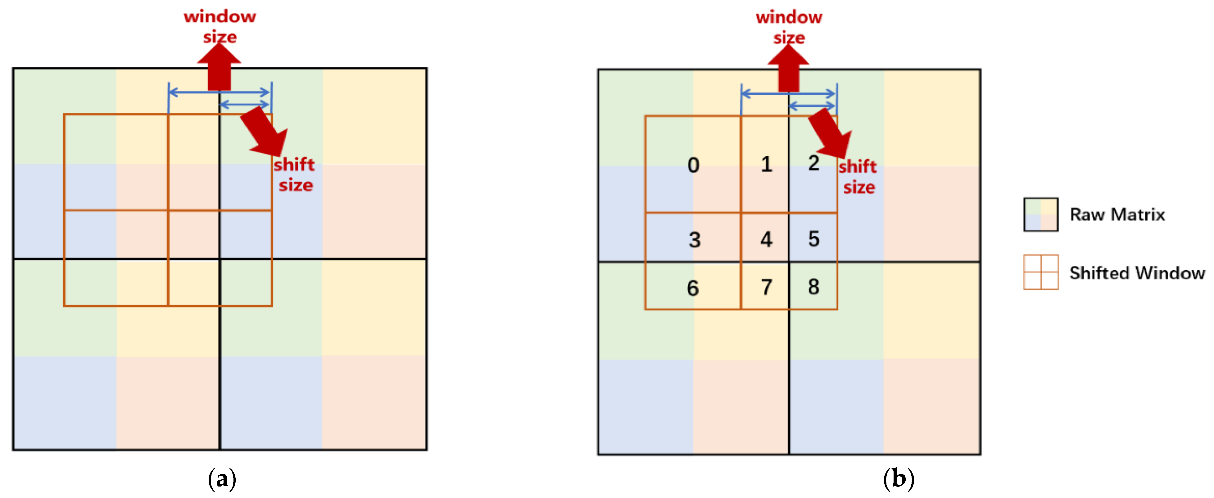
2.2.3. Shifted Window Partitioning in Successive Blocks

Since the absence of information exchange between non-overlapping windows undoubtedly limits their modeling capabilities, cross-window connections are introduced. In two successive Swin Transformer blocks, this technique alternates W-MSA with SW-MSA. The shifted window division method makes the connection between adjacent non-overlapping windows in the upper layer and increases the perceptual field of view.
With the shifted structure, the Swin Transformer blocks are calculated as follows.
z ^ l = W M S A ( L N ( z l 1 ) ) + z l 1 ,
z l = M L P ( L N ( z ^ l ) ) + z ^ l ,
z ^ l + 1 = S W M S A ( L N ( z l ) ) + z l ,
z l + 1 = M L P ( L N ( z ^ l + 1 ) ) + z ^ l + 1 ,
where z ^ l and zl denote the output features of the (S)W-MSA module and the MLP module for block, respectively; W-MSA and SW-MSA are window-based multihead self-attention algorithms that use normal and shifted window partitioning configurations, respectively.

2.2.4. Multihead Self-Attention

Multihead attention mechanism is used for migration from Transformer to vision. The specific formula is as follows.
A t t e n t i o n ( Q , K , V ) = s o f t max ( Q K T d + B ) V                         ( Q , K , V R M 2 + d )
where B is the relative position parameter, which is introduced similarly to the position embedding in Transformer. d is the size of the dimension corresponding to each head, which serves to balance the size of QKT and B. Q, K, V calculation: for the incoming window information, the corresponding query, key, and value values are obtained after a linear layer.

2.2.5. Third Stage

The above introduces how to use a Swin Transformer to extract features, and finally, we used a Swin Transformer to complete the mission of classification and segmentation, respectively [29].
The third stage contains two downstream missions: classification and segmentation. For the classification mission, the output dimension is specified as the number of classifications (in our experiments, there were two categories, with and without nodules), and then the output is passed through softmax to obtain the final classification probability. For the segmentation mission, semantic segmentation is made here as the backbone for extracting image features.

2.3. Architecture Variants

We used Swin Transformer’s base model, Swin-B, to have a model size and computing complexity similar to ViT-B/DeiT-B. We only used some of the Swin-T and Swin-S models for training due to experimental equipment restrictions. Swin-T and Swin-S are models with 0.25, 0.5, and 2 times the computational complexity, respectively. Swin-T and Swin-S are equivalent in complexity to ResNet-50 (DeiT-S) and ResNet-101, respectively. By default, the window size is set at M = 7. For all tests, the query dimension of each head is d = 32, and the expansion layer of each MLP is =4. These model versions’ architecture hyper-parameters are:
  • Swin-T: C = 96, layer numbers = {2, 2, 6, 2};
  • Swin-S: C = 96, layer numbers = {2, 2, 18, 2};
  • Swin-B: C = 128, layer numbers = {2, 2, 18, 2}.
where C is the channel number of the hidden layers in the first stage.

2.4. Loss Function

The loss function for the classification mission is as follows:
L = 1 N i L i = 1 N i c = 1 M y i c log ( p i c )
where M is the number of categories and yic is the symbolic function (0 or 1). If the true category of the sample i is equal to 2, take 1; otherwise, take 0. pij is the predicted probability that the observed sample i belongs to category 2.
For the segmentation mission, its loss function is Equation (6), classified by pixel.

3. Experiments

3.1. Datasets

3.1.1. Classification Dataset

The LUNA16 dataset is a public dataset marked by four experienced thoracic radiologists on nodules, which is a part of LIDC/IDRI [30]. The dataset is composed of 888 low-dose lung CT images, each containing a series of axial sections of the thorax. The LUNA16 dataset has been curated to include only annotations that have been agreed upon by multiple radiologists, and tumors smaller than 3 mm have been removed. This simplifies the training process as such small tumors can be difficult for even experienced doctors to identify. The number of slices per image can vary depending on factors such as the imaging machine, the thickness of each layer, and the patient. The original images are three-dimensional and consist of a series of axial sections of the thorax. These 3D images are comprised of a varying number of 2D images.
To prepare benign and malignant classification data of pulmonary nodules:
Each nodule is labeled on the 3D image. Our task is to obtain the part with nodules from the 3D image and divide it into 2D images. First, we obtained the center coordinates of all nodes in the annotation file, took the (48,48,48) dimensional area image with these coordinates as the 3D image of the candidate lung nodules, and then sliced them one at a time along with the x-direction, y-direction, and z-direction to obtain our dataset. The current dataset exhibits a marked class imbalance, where the number of positive samples (lung nodules) is significantly lower in comparison to the negative samples (non-lung nodules). Specifically, there are 1351 positive samples and 549,714 negative samples. This disparity in class population presents a challenge in the development of accurate models for detecting lung nodules. Next, we performed data augmentation. For 1351 lung nodule pictures, we performed a 40-fold expansion (rotation, panning, flipping, etc.). There was also a 20% random selection of 549,714 lung nodule photographs. To make the dataset suitable for Swin Transformer, we batch-loaded all the original 3D datasets and converted them to RGB images [31].
For better experiments, we divided the data into three categories: training, testing, and validation. In the training set, the ratio of positive to negative samples is 6:1; in the test set, the ratio of positive to negative samples is 1:1; and in the validation set, the ratio of positive to negative samples is 1.2:1. As seen in Table 1, we obtained 20,565 images in the training dataset, 2571 images in the validated dataset, and 7076 images in the test dataset.

3.1.2. Segmentation Dataset

For the segmentation mission, we used the MSD dataset [30]. This dataset contains 60 patients, corresponding to 96 CT, and is manually labeled with contour information. The original dataset has a train set and test set in two parts, so we marked the label according to the signature file in the original dataset. Additionally, each part contains two classes: 0 and 1.
The first task is to cut the 3D images of the original dataset in the x-direction, y-direction, and z-direction. To solve this problem, we sliced the images and labels in three directions (x-direction, y-direction, and z-direction), as shown in Figure 3.
We divided the above-processed data into train, test, and validation. As to the specific division of the dataset, we adopted an 8:1:1 ratio. Finally, as seen in Table 1, we obtained 22,009 images in the training dataset, 1702 images in the validated dataset, and 1702 images in the test dataset, which can ensure our experiment reaches relatively high accuracy.

3.2. Metric Evaluation

‘top-1 acc’ and ‘top-5 acc’ are commonly employed to measure the performance of a classifier on the validation set. The term ‘top’ refers to the rank of a class in terms of its predicted probability of being the true label.
Top-1 acc, also known as single-label accuracy, measures the accuracy of the classifier in assigning the correct class to an image based on the highest predicted probability among all classes. In other words, it evaluates the classifier’s ability to correctly identify the class with the highest predicted probability as the true label.
Top-5 acc, on the other hand, assesses the accuracy of the classifier in correctly identifying the true label among the top 5 classes with the highest predicted probabilities. This metric reflects the classifier’s ability to correctly identify the true label even if it is not the class with the highest predicted probability.
Both of these metrics are useful in evaluating the performance of a medical image classifier, and the choice between using top-1 acc or top-5 acc may depend on the specific requirements of the problem at hand and the desired level of accuracy for class predictions.
For semantic segmentation of medical images, we used mIoU to evaluate the results, which is a common evaluation method. IoU is calculated for all categories, and then the mean of each category is calculated to obtain a global evaluation. The specific calculation formula of mIoU is:
M I o U = 1 K + 1 i = 1 k p i i j = 0 k p i j + j = 0 k p j i p i i
Where i denotes the true value; j denotes the predicted value; pij denotes the prediction of i to j; k denotes the number of categories; and pii is the number of true samples, which in this paper is the number of successful predictions with nodal samples.
In addition, we used the built-in evaluation metrics mAcc and aAcc from mmseg [32,33] to measure the accuracy of the training results.

3.3. Experiment Result

3.3.1. Classification
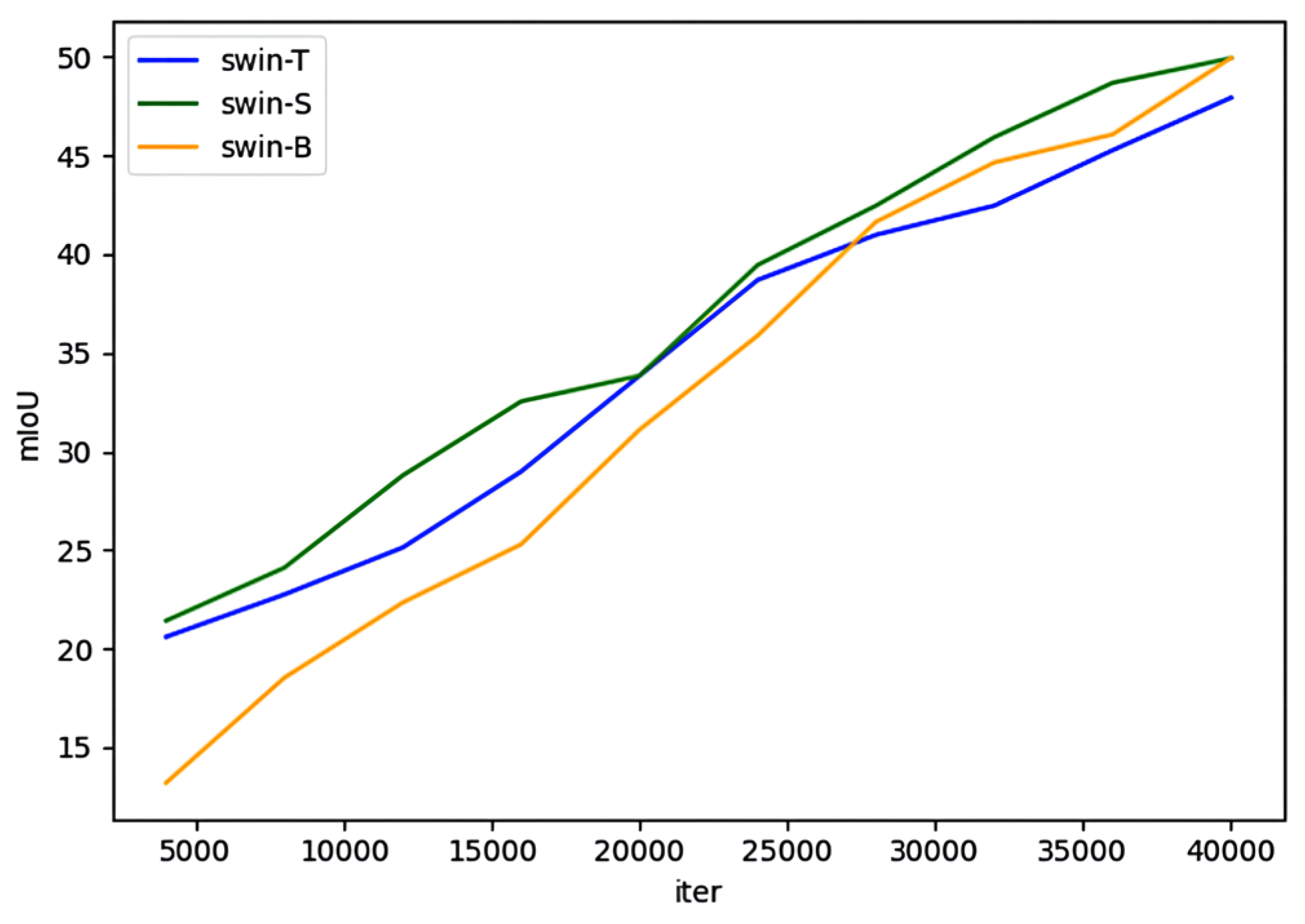
We benchmarked the Swin Transformer on LUNA16, which involves 12.6 MB training images and 1.58 MB validation images from 2 classes (0 or 1). Considering the particularity of the medical CT dataset, we adopted two training settings to compare, which include (1) regular training; (2) fine-tuning with pre-training. The main instruction is as follows.
For regular training: our normal training setup in LUNA16 is as follows [15]. A cosine decay learning rate scheduler uses an AdamW [34] for 300 epochs and linear warm-up for 20 epochs. We used a batch size of 28, a 0.001 starting learning rate, and a 0.05 weight decay. Although the training includes the majority of augmentation and regularization as well as EMA [35], it does not improve performance.
Figure 3 compares Swin-T, Swin-S, and Swin-B in two different resolutions (we denoted these two models, respectively, according to their resolution as Swin-B_224 and Swin-B_384) when it comes to the loss and accuracy for the missions of lung nodule classification. As seen in Figure 4a, the overall curve shows a downward trend, among which the Swin-T curve fluctuates significantly, and the Swin-B_224 curve has the lowest fluctuation range and the best stability. As seen in Figure 4b, Swin-T has the highest accuracy of training results, while the other models cannot achieve good training results, which is caused by the different fitness of dataset sizes for different models and the lack of pre-training. Mean-while, there is a gradient explosion because the loss values of the training results gradually become NAN. This result is caused by not being pre-trained.
Table 2 details the result of the comparison of different backbones in regular training on LUNA16 classification. The resolutions of the models are shown in Table 2, among which the Swin-B model contains two different resolutions. The performance of the validation set in our study is evaluated using two measures of accuracy: top-1 acc and top-5 acc. Top-1 acc quantifies the ability of the classifier to correctly assign the true label to an image, given the highest predicted probability of all classes. Conversely, top-5 acc evaluates the classifier’s ability to correctly identify the true label among the top 5 classes with the highest predicted probabilities. Both of these metrics provide insights into the classifier’s capability to accurately predict the true labels of images in the validation set. The Swin Transformer model shows the best training results, with high accuracy and small parameters. This may be due to the gradient explosion and underfitting. The accuracy of Swin-T (82.3%) is higher than the other two models, ViT-B/16 and ViT-L/16, during regular training.
In terms of pre-training and fine-tuning, Figure 5 compares loss and accuracy for Swin-B at two different resolutions (we denoted these two models, respectively, according to their resolution as Swin-B_224 and Swin-B_384) in pre-training. As seen in Figure 5a, the curve showed a downward trend. The initial value of the Swin-B_224 model was high, and the range of decrease was large, while the loss value of the other model had a relatively small change range. The accuracy of the two models is depicted in in Figure 5b. We can see that the accuracy of the two models finally reaches a good level after pre-training.
Table 3 details the result of a comparison of different backbones. The table shows that the pre-training model helps improve accuracy to some extent. Additionally, we compared the experimental results of Swin-B with those of ViT and found that the training results of Swin-B were better. The two resolutions of Swin-B in Figure 5b refer to specific types of pre-training models [30].
To compare the results of the experiment, we pre-trained LUNA16 and fine-tuned it. We adopted a linear decay learning rate scheduler with a 5-epoch linear warm-up to run an AdamW optimizer for 30 epochs. We used a batch size of 28, a constant learning rate of 10−5, and a weight decay of 10−8.
We evaluated the performance of the models in regular training and observed that only the Swin-T model achieved a high level of accuracy, with a maximum of 82.3%. The 1-top accuracy of Swin-S and Swin-B, on the other hand, was significantly lower at 17.736%, and their maximum accuracy was only 17.74%.
Differently, the result of pre-training and fine-tuning is an idol. As we expected in Table 3, the test images’ max accuracy reached 82.3%, and the gradient explosion phenomenon disappeared.
In addition, we added comparison experiments to compare the Swin Transformer model with ViT. In regular training, the advantage of the Swin Transformer is not particularly significant, and only good results are achieved in the training accuracy of Swin-T compared to ViT. In pre-training, our model Swin-B achieved 82.26% top-1 acc, which is 2.529% higher than ViT.
Figure 6 shows the comparison of the loss curve results of Swin-B_224 and Swin-B_384 models with or without pre-training. The curve decreases rapidly during 0–200, then changes slowly during 200–2000 again, and stabilizes after 2000. When the two models are stable, the fluctuation range of the loss curve of the pre-trained model is small.
In addition, we can see the parameter comparison of the four models in Figure 7. As seen in Figure 7a, the two resolutions of Swin-B have the same parameters. However, as seen in Figure 7b, the Swin-B model with a resolution of 384 takes the longest computational time and has the highest computational complexity.

3.3.2. Segmentation

Due to its high efficiency, we employed UperNet [37] in mmseg [38]. The model comes in three sizes: tiny, small, and base. In segmentation missions, we employed pre-training. We used the AdamW [20] optimizer in training, with a learning rate of 6 × 10⁻⁵, a weight decay of 0.01, a linear learning rate decay scheduler, and a linear warmup of 1500 iterations. Models were trained on a single GPU for 40 K encounters as a limitation of the experiment. We used the default mmseg settings of random horizontal flipping, random rescaling within the ratio range [0.5, 2.0], and random photometric distortion for augmentations [23]. For all Swin Transformer models, a stochastic depth with a ratio of 0.2 was used.
At the beginning of the segmentation experiments, we found that the loss quickly goes to zero. After repeated changes, the loss still showed no improvement. Finally, we determined that the problem was over-fitting. To solve this sticky problem, we employed data augmentation techniques to generate more similar data from restricted datasets, enrich the distribution of training data, and improve the model’s generalizability. We used the data augmentation library to rotate the picture counterclockwise randomly, flip it horizontally, flip it up and down, and enlarge the image at the same scale. The data augmentation image styles are shown in Figure 8.
We employed a pre-training strategy to train the dataset to gain the required results because of the big dataset. The pre-training model [23] we used here is the same one used in the classification experiment. Table 4 lists the mIoU, model size (#param), and FLOPs for different method/backbone pairs. The mAcc and aAcc of the three models all reached over 95%. Among them, the Swin-B model has the most outstanding performance, with an accuracy of 99.91%. We used the built-in evaluation metrics mAcc and aAcc from mmseg [38] to measure the accuracy of the training results. Comparing Swin Transformer with the two sets of comparison experiments we set up, we found that Swin-S is +5.01 mIoU higher compared to ResNet-101 and +5.82 mIoU higher compared to DeiT-S.
The loss curves of the three models are shown in Figure 9. The curves drop rapidly in the process of 0–750, then change slowly in the process of 750–1500, and stabilize after 2000. All three models have small loss values as they converge to stability.
In Figure 10, we can see the comparison of the accuracy of the training results of the three models. Among them, the accuracy of Swin-B is the best, and the accuracy of Swin-T is the worst. The Swin-T curve fluctuates the most, and the Swin-B curve is the smoothest.
Figure 11 shows a global evaluation using the mIoU curve, and the Swin-S and Swin-B models reveal the best effect. The mIoU of Swin-T is the worst.
In addition, we can attain a clear comparison of model parameters params and flops from viewing Figure 12. We can see that the larger the model size is, the larger the values of params and flops are.

4. Discussion

Transformers have made great progress in traditional image-processing technology. In this paper, we innovatively propose a segmentation method based on an efficient transformer and apply it to medical image analysis. It is a new visual converter that generates hierarchical feature representations with linear computing complexity about the size of the input image. We completed two missions of Swin Transformer for CT image classification on the LUNA16 dataset and segmentation of the MSD dataset. Experiments comparing with the ViT model in the classification mission and with ResNet-101 and DeiT-S in the segmentation mission were conducted to show that Swin Transformer has good results in specific lung cancer detection areas.
In the future, we will improve the Swin Transformer to make it more universally applicable in the field of medical imaging. In addition, the dataset in this paper was pre-processed and converted into 2D images. Due to the prevalence of 3D medical images, in the future, we will study how Swin Transformer can be applied in 3D medical image classification and segmentation.

Author Contributions

Conceptualization, supervision, methodology, project administration, R.S.; investigation, resources, writing—original draft preparation, R.S.; Data curation, validation, Writing—review & editing, Y.P.; Supervision, Funding acquisition, W.L. All authors have read and agreed to the published version of the manuscript.

Funding

The National Key R&D Program of China (2020AAA0105200) and the National Natural Science Foundation of China (No. 61972040).

Data Availability Statement

The dataset used to support the findings of this study is available from the corresponding author upon request.

Acknowledgments

We are very grateful to Hanyu Zhao for his help in writing, reviewing, editing and obtaining funds.

Conflicts of Interest

The authors declare that there is no conflict of interest regarding the publication of this paper.

References

  1. Hvidtfeldt, U.A.; Severi, G.; Andersen, Z.J.; Atkinson, R.; Bauwelinck, M.; Bellander, T.; Boutron-Ruault, M.-C.; Brandt, J.; Brunekreef, B.; Cesaroni, G.; et al. Long-term low-level ambient air pollution exposure and risk of lung cancer–A pooled analysis of 7 European cohorts. Environ. Int. 2021, 146, 106249. [Google Scholar] [CrossRef] [PubMed]
  2. Huang, Y.; Zhu, M.; Ji, M.; Fan, J.; Xie, J.; Wei, X.; Jiang, X.; Xu, J.; Chen, L.; Yin, R.; et al. Air pollution, genetic factors, and the risk of lung cancer: A prospective study in the UK Biobank. Am. J. Respir. Crit. Care Med. 2021, 204, 817–825. [Google Scholar] [CrossRef] [PubMed]
  3. Prabhakar, B.; Shende, P.; Augustine, S. Current trends and emerging diagnostic techniques for lung cancer. Biomed. Pharmacother. 2018, 106, 1586–1599. [Google Scholar] [CrossRef] [PubMed]
  4. Peng, H.; Huang, S.; Chen, S.; Li, B.; Geng, T.; Li, A.; Jiang, W.; Wen, W.; Bi, J.; Liu, H.; et al. A length adaptive algorithm-hardware co-design of transformer on fpga through sparse attention and dynamic pipelining. In Proceedings of the 59th ACM/IEEE Design Automation Conference, San Antonio, Texas, USA, 16–19 May 2022; pp. 1135–1140. [Google Scholar]
  5. LeCun, Y.; Kavukcuoglu, K.; Farabet, C. Convolutional networks and applications in vision. In Proceedings of the 2010 IEEE International Symposium on Circuits and Systems, Paris, France, 30 May–2 June 2010; pp. 253–256. [Google Scholar]
  6. Wei, X.; Saha, D. KNEW: Key Generation using NEural Networks from Wireless Channels. In Proceedings of the 2022 ACM Workshop on Wireless Security and Machine Learning, San Francisco, CA, USA, 10–14 July 2022; pp. 45–50. [Google Scholar]
  7. Kuan, K.; Ravaut, M.; Manek, G.; Chen, H.; Lin, J.; Nazir, B.; Chen, C.; Howe, T.C.; Zeng, Z.; Chandrasekhar, V. Deep learning for lung cancer detection: Tackling the kaggle data science bowl 2017 challenge. arXiv 2017, arXiv:1705.09435. [Google Scholar]
  8. Zou, Z.; Careem, M.; Dutta, A.; Thawdar, N. Joint Spatio-Temporal Precoding for Practical Non-Stationary Wireless Channels. IEEE Trans. Commun. 2023. [Google Scholar] [CrossRef]
  9. Zou, Z.; Careem, M.; Dutta, A.; Thawdar, N. Unified characterization and precoding for non-stationary channels. In Proceedings of the ICC 2022-IEEE International Conference on Communications, Seoul, Republic of Korea, 16–20 May 2022; pp. 5140–5146. [Google Scholar]
  10. Shen, G.; Zeng, W.; Han, C.; Liu, P.; Zhang, Y. Determination of the average maintenance time of CNC machine tools based on type II failure correlation. Eksploatacja i Niezawodność 2017, 19. [Google Scholar] [CrossRef]
  11. Moradi, P.; Jamzad, M. Detecting lung cancer lesions in CT images using 3D convolutional neural networks. In Proceedings of the 2019 4th International Conference on Pattern Recognition and Image Analysis (IPRIA), Tehran, Iran, 6–7 March 2019; pp. 114–118. [Google Scholar]
  12. Shen, W.; Zhou, M.; Yang, F.; Yang, C.; Tian, J. Multi-scale convolutional neural networks for lung nodule classification. In International Conference on Information Processing in Medical Imaging; Springer: Cham, Switzerland, 2015; pp. 588–599. [Google Scholar]
  13. Xie, Y.; Xia, Y.; Zhang, J.; Song, Y.; Feng, D.; Fulham, M.; Cai, W. Knowledge-based collaborative deep learning for benign-malignant lung nodule classification on chest CT. IEEE Trans. Med. Imaging 2018, 38, 991–1004. [Google Scholar] [CrossRef] [PubMed]
  14. Peng, H.; Gurevin, D.; Huang, S.; Geng, T.; Jiang, W.; Khan, O.; Ding, C. Towards Sparsification of Graph Neural Networks 2022 IEEE 40th International Conference on Computer Design (ICCD). In Proceedings of the 2022 IEEE 40th International Conference on Computer Design (ICCD), Olympic Valley, CA, USA, 23–26 October 2022; pp. 272–279. [Google Scholar] [CrossRef]
  15. Touvron, H.; Cord, M.; Douze, M.; Massa, F.; Sablayrolles, A.; Jegou, H. Training data-efficient image transformers & distillation through attention. In Proceedings of the International Conference on Machine Learning, Virtual, 18–24 July 2021; pp. 10347–10357. [Google Scholar]
  16. Du, X.; Tang, S.; Lu, Z.; Wet, J.; Gai, K.; Hung, P.C.K. A Novel Data Placement Strategy for Data-Sharing Scientific Workflows in Heterogeneous Edge-Cloud Computing Environments. In Proceedings of the 2020 IEEE International Conference on Web Services (ICWS), Beijing, China, 19–23 October 2020; pp. 498–507. [Google Scholar]
  17. Fu, J.; Liu, J.; Wang, Y.; Li, Y.; Bao, Y.; Tang, J.; Lu, H. Adaptive context network for scene parsing. In Proceedings of the IEEE/CVF International Conference on Computer Vision, Seoul, Republic of Korea, 27 October–2 November 2019; pp. 6748–6757. [Google Scholar]
  18. Zhou, J.; Xiong, W.; Tian, Q.; Qi, Y.; Liu, J.; Leow, W.K.; Han, T.; Venkatesh, S.K.; Wang, S. Semi-automatic segmentation of 3D liver tumors from CT scans using voxel classification and propagational learning. MICCAI Workshop 2008, 41, 43. [Google Scholar] [CrossRef]
  19. Wang, S.; Zhou, M.; Gevaert, O.; Tang, Z.; Dong, D.; Liu, Z.; Jie, T. A multi-view deep convolutional neural networks for lung nodule segmentation. In Proceedings of the 2017 39th Annual International Conference of the IEEE Engineering in Medicine and Biology Society (EMBC), Jeju, Republic of Korea, 11–15 July 2017; pp. 1752–1755. [Google Scholar]
  20. Loshchilov, I.; Hutter, F. Decoupled Weight Decay Regularization. In Proceedings of the 7th International Conference on Learning Representations, New Orleans, LA, USA, 6–9 May 2019. [Google Scholar]
  21. Khan, S.; Naseer, M.; Hayat, M.; Zamir, S.W.; Khan, F.S.; Shah, M. Transformers in vision: A survey. ACM Comput. Surv. (CSUR) 2022, 54, 1–41. [Google Scholar] [CrossRef]
  22. Zhou, D.; Kang, B.; Jin, X.; Yang, L.; Lian, X.; Jiang, Z.; Hou, Q.; Feng, J. Deepvit: Towards deeper vision transformer. arXiv 2021, arXiv:2103.11886. [Google Scholar]
  23. Liu, Z.; Lin, Y.; Cao, Y.; Hu, H.; Wei, Y.; Zhang, Z.; Lin, S.; Guo, B. Swin transformer: Hierarchical vision transformer using shifted windows. In Proceedings of the IEEE/CVF International Conference on Computer Vision, Montreal, QC, Canada, 10–17 October 2021; pp. 10012–10022. [Google Scholar]
  24. Cao, H.; Wang, Y.; Chen, J.; Jiang, D.; Zhang, X.; Tian, Q.; Wang, M. Swin-unet: Unet-like pure transformer for medical image segmentation. arXiv 2021, arXiv:2105.05537. [Google Scholar]
  25. Zhang, Y.; Mu, L.; Shen, G.; Yu, Y.; Han, C. Fault diagnosis strategy of CNC machine tools based on cascading failure. J. Intell. Manuf. 2019, 30, 2193–2202. [Google Scholar] [CrossRef]
  26. Ning, X.; Tian, W.; He, F.; Bai, X.; Sun, L.; Li, W. Hyper-sausage coverage function neuron model and learning algorithm for image classification. Pattern Recognit. 2023, 136, 109216. [Google Scholar] [CrossRef]
  27. Cai, W.; Liu, D.; Ning, X.; Wang, C.; Xie, G. Voxel-based three-view hybrid parallel network for 3D object classification. Displays 2021, 69, 102076. [Google Scholar] [CrossRef]
  28. Chen, Z.; Silvestri, F.; Tolomei, G.; Wang, J.; Zhu, H.; Ahn, H. Explain the Explainer: Interpreting Model-Agnostic Counterfactual Explanations of a Deep Reinforcement Learning Agent. IEEE Trans. Artif. Intell. 2022. [Google Scholar] [CrossRef]
  29. Zhang, L.; Sun, L.; Li, W.; Zhang, J.; Cai, W.; Cheng, C.; Ning, X. A joint bayesian framework based on partial least squares discriminant analysis for finger vein recognition. IEEE Sens. J. 2021, 22, 785–794. [Google Scholar] [CrossRef]
  30. Armato, S.G., III; McLennan, G.; Bidaut, L.; McNitt-Gray, M.F.; Meyer, C.R.; Reeves, A.P.; Zhao, B.; Aberle, D.R.; Henschke, C.I.; Hoffman, E.A.; et al. The lung image database consortium (LIDC) and image database resource initiative (IDRI): A completed reference database of lung nodules on CT scans. Med. Phys. 2011, 38, 915–931. [Google Scholar] [CrossRef] [Green Version]
  31. He, F.; Bai, K.; Zong, Y.; Zhou, Y.; Jing, Y.; Wu, G.; Wang, C. Makeup transfer: A review. IET Comput. Vis. 2022. [Google Scholar] [CrossRef]
  32. Simpson, A.L.; Antonelli, M.; Bakas, S.; Bilello, M.; Farahani, K.; Van Ginneken, B.; Kopp-Schneider, A.; Landman, B.A.; Litjens, G.; Menze, B.; et al. A large annotated medical image dataset for the development and evaluation of segmentation algorithms. arXiv 2019, arXiv:1902.09063. [Google Scholar]
  33. Wang, Y.; Du, X.; Lu, Z.; Duan, Q.; Wu, J. Improved LSTM-based Time-Series Anomaly Detection in Rail Transit Operation Environments. IEEE Trans. Ind. Inform. 2022, 18, 9027–9036. [Google Scholar] [CrossRef]
  34. Kingma, D.P.; Ba, J. Adam: A method for stochastic optimization. arXiv 2014, arXiv:1412.6980. [Google Scholar]
  35. Polyak, B.T.; Juditsky, A.B. Acceleration of stochastic approximation by averaging. SIAM J. Control. Optim. 1992, 30, 838–855. [Google Scholar] [CrossRef] [Green Version]
  36. Dosovitskiy, A.; Beyer, L.; Kolesnikov, A.; Weissenborn, D.; Zhai, X.; Unterthiner, T.; Dehghani, M.; Minderer, M.; Heigold, G.; Gelly, S.; et al. An image is worth 16x16 words: Transformers for image recognition at scale. arXiv 2020, arXiv:2010.11929. [Google Scholar]
  37. Xiao, T.; Liu, Y.; Zhou, B.; Jiang, Y.; Sun, J. Unified perceptual parsing for scene understanding. In Proceedings of the European Conference on Computer Vision (ECCV), Munich, Germany, 8–14 September 2018; pp. 418–434. [Google Scholar]
  38. Contributors, M. Mmsegmentation, an Open Source Semantic Segmentation Toolbox. 2020. Available online: https://github.com/open-mmlab/mmsegmentation (accessed on 23 December 2022).
Figure 1. Mask slice and after mask slicing. (a) Mask slice; (b) After mask slicing.
Electronics 12 01024 g001
Figure 2. (a) Lung cancer detection process (Swin-T); (b) UPerNet structure in segmentation missions.
Electronics 12 01024 g002aElectronics 12 01024 g002b
Figure 3. The section of lung nodule from three directions (the areas marked by red circles are where the lung nodules are located).
Electronics 12 01024 g003
Figure 4. Comparison of loss and accuracy for different models in training. (a) Loss for training; (b) Accuracy for training.
Electronics 12 01024 g004
Figure 5. Comparison of loss and accuracy for different models in pre-training. (a) Loss for pre-training; (b) Accuracy for pre-training.
Electronics 12 01024 g005
Figure 6. Comparison of loss for Swin-B with different image sizes. (a) Comparison of loss for Swin-B with image size of 224 in training and pre-training; (b) Comparison of loss for Swin-B with image size of 384 in training and pre-training.
Electronics 12 01024 g006
Figure 7. Comparison of params and flops in classification mission. (a) Comparison of params; (b) Comparison of flops.
Electronics 12 01024 g007
Figure 8. A sample of the data augmentation images.
Electronics 12 01024 g008
Figure 9. Comparison of loss for different models.
Electronics 12 01024 g009
Figure 10. Comparison of accuracy for different models.
Electronics 12 01024 g010
Figure 11. Comparison of mIoU for different models.
Electronics 12 01024 g011
Figure 12. Comparison of params and flops in segmentation mission. (a) Comparison of params; (b) Comparison of flops.
Electronics 12 01024 g012
Table 1. Dataset indication.
ClassificationSegmentation
Dataset typeLUNA16MSD
Train data20,56522,009
Validate data25711702
Test data70761702
Space usage18.6 MB5.48 GB
Table 2. Comparison of different backbones in regular training on LUNA16 classification.
Method ResolutionTop-1 AccTop-5 AccMax Acc#ParamsFLOPs
Swin-T [23]224282.2682.2682.328 M4.5 G
Swin-S [23]224219.7619.7619.850 M8.7 G
Swin-B [23]224217.73617.73617.788 M15.4 G
Swin-B [23]384250.050.050.088 M47.1 G
ViT-B/16 [36]384268.5668.5668.686 M55.4 G
ViT-L/16 [36]384269.4369.4369.4307 M190.7 G
Table 3. Comparison of different backbones in pre-training and fine-tuning on LUNA16 classification.
Method ResolutionTop-1 AccTop-5 AccMax Acc#ParamsFLOPs
Swin-B
Swin-B
2242
3842
82.264
82.260
82.264
82.260
82.3
82.3
88 M
88 M
15.4 G
47.1 G
ViT-B/16 [36]384279.73179.73179.786 M55.4 G
ViT-L/16 [36]384279.89079.89079.9307 M190.7 G
Table 4. Comparison of different backbones in pre-training on MSD segmentation.
Backbone Method#ParmasFLOPsmIoUmAccaAcc
Swin-T [23]UPerNet60 M945 G47.9395.8795.87
Swin-S [23]UPerNet81 M1038 G49.9499.8799.87
Swin-B [23]UPerNet121 M1188 G49.9599.9199.91
ResNet-101UperNet86 M1029 G44.9392.2592.25
DeiT-S [15]UPerNet52 M1099 G44.1290.7590.75
Disclaimer/Publisher’s Note: The statements, opinions and data contained in all publications are solely those of the individual author(s) and contributor(s) and not of MDPI and/or the editor(s). MDPI and/or the editor(s) disclaim responsibility for any injury to people or property resulting from any ideas, methods, instructions or products referred to in the content.

