

LiDAR SLAM with a Wheel Encoder in a Featureless Tunnel Environment

Abstract
:1. Introduction
- We modify a state-of-the-art LiDAR SLAM algorithm by incorporating additional wheel encoder sensor data from an unmanned ground vehicle by employing an EKF to improve the localization and mapping accuracy of the SLAM framework in a dark, featureless tunnel environment.
- We improve the LiDAR SLAM algorithm localization and mapping accuracy by implementing additional sensor data from the ground vehicle’s wheel encoders.
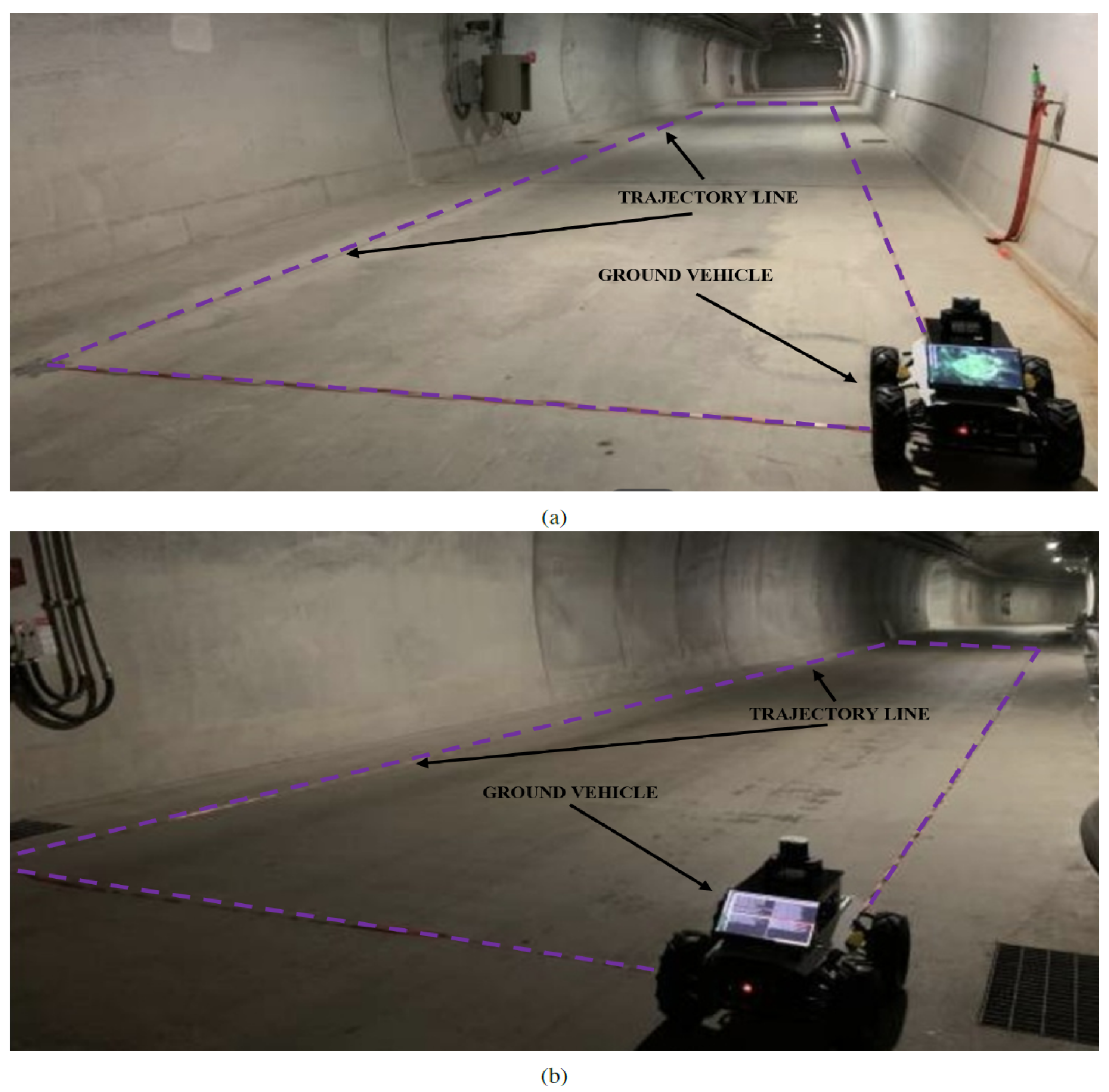
- We performed extensive experiments in flat and inclined terrain sections of the tunnel environment to evaluate the LiDAR SLAM performance.
2. Related Work
3. Proposed Method
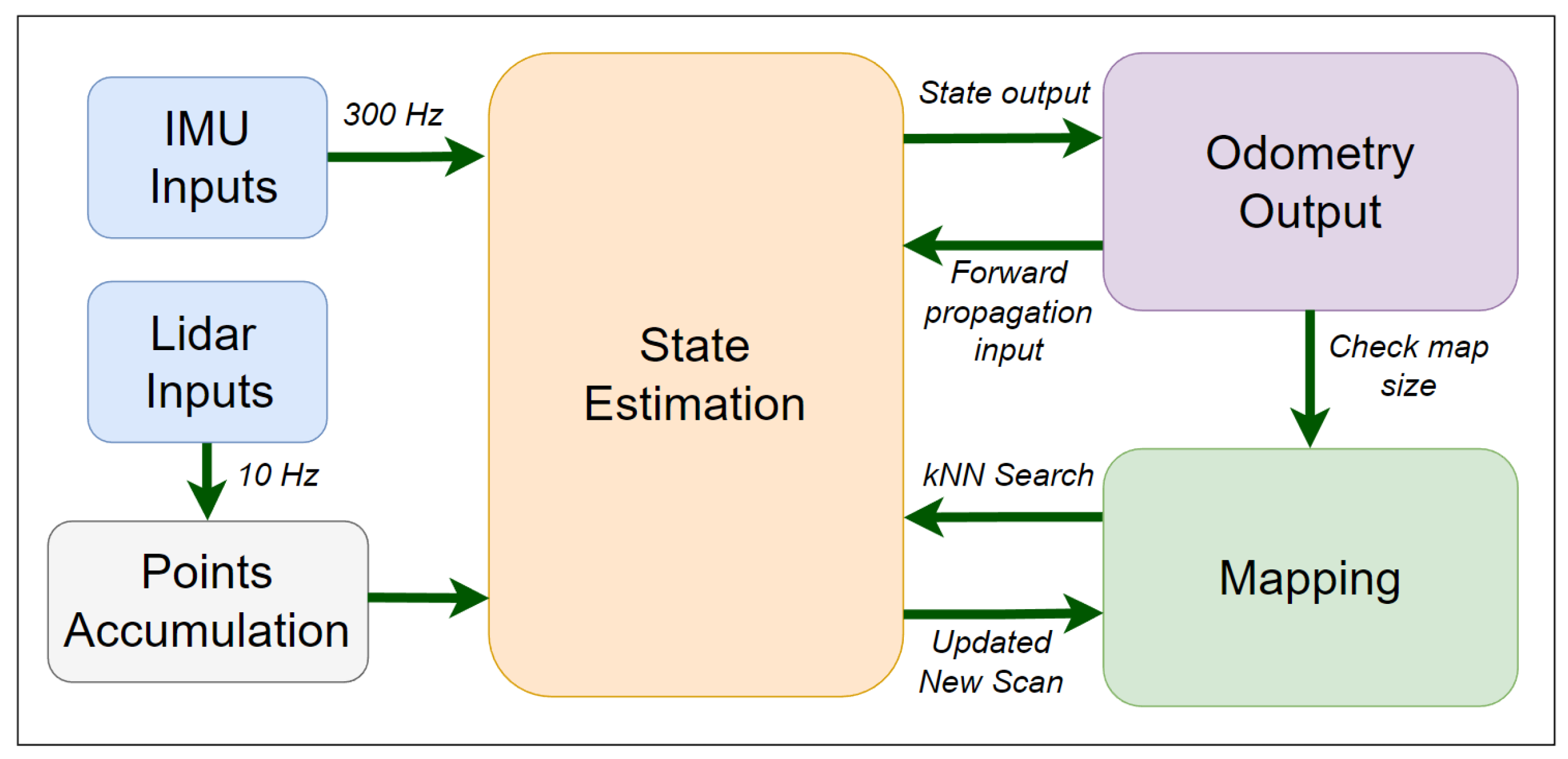
3.1. FAST-LIO2 Overview
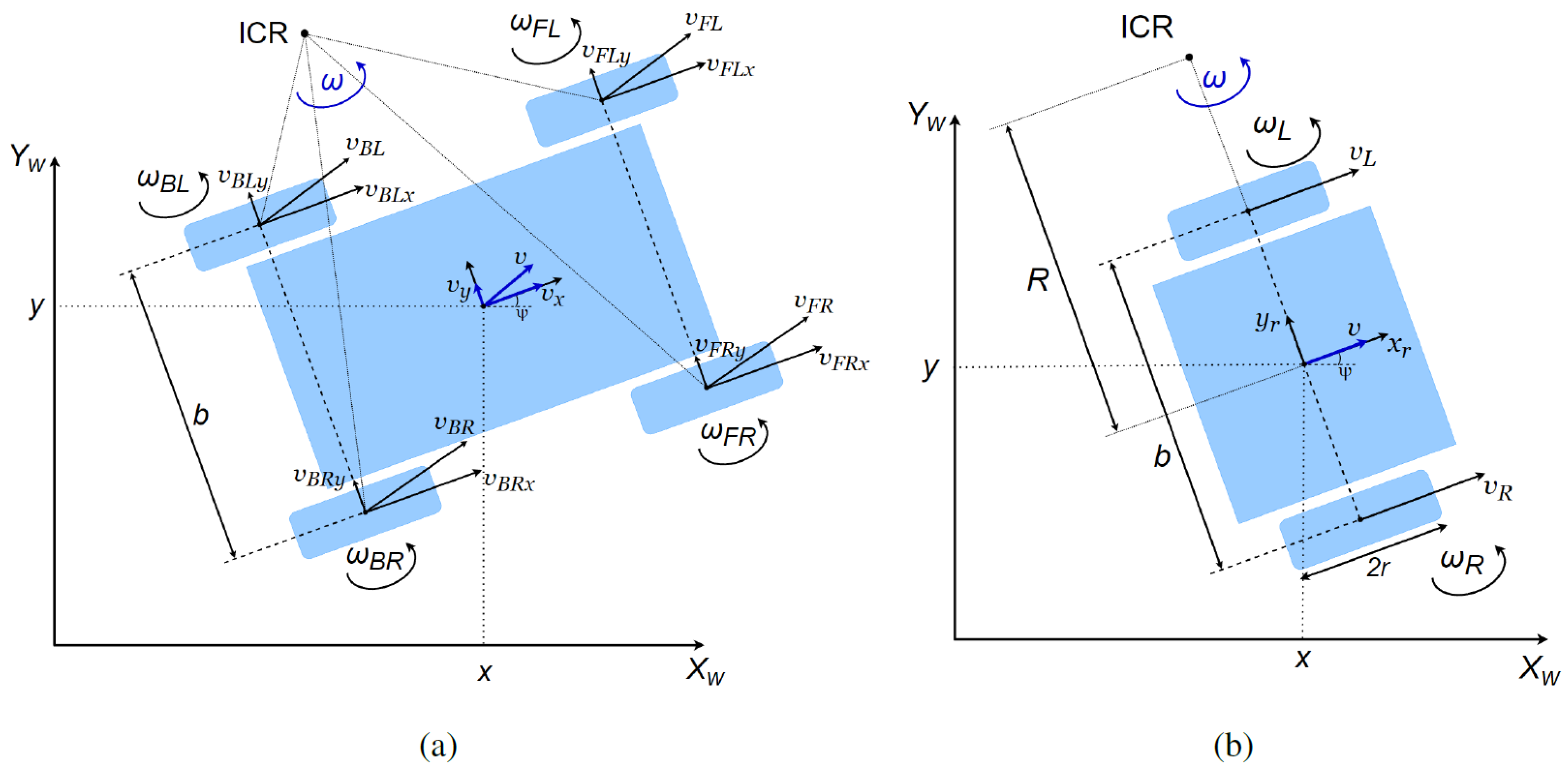
3.2. Motion Model
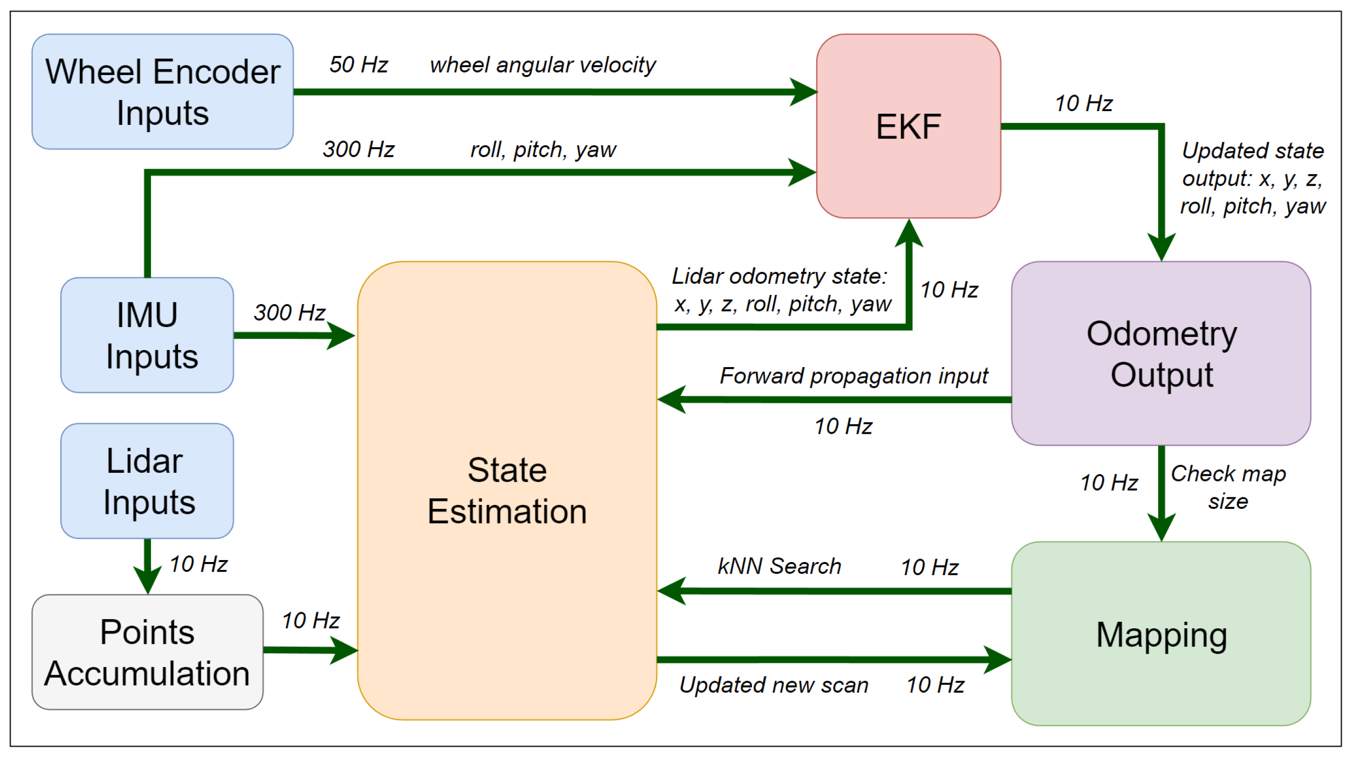
3.3. EKF
3.4. Wheel Encoder Aided FAST-LIO2
4. Experiment and Results
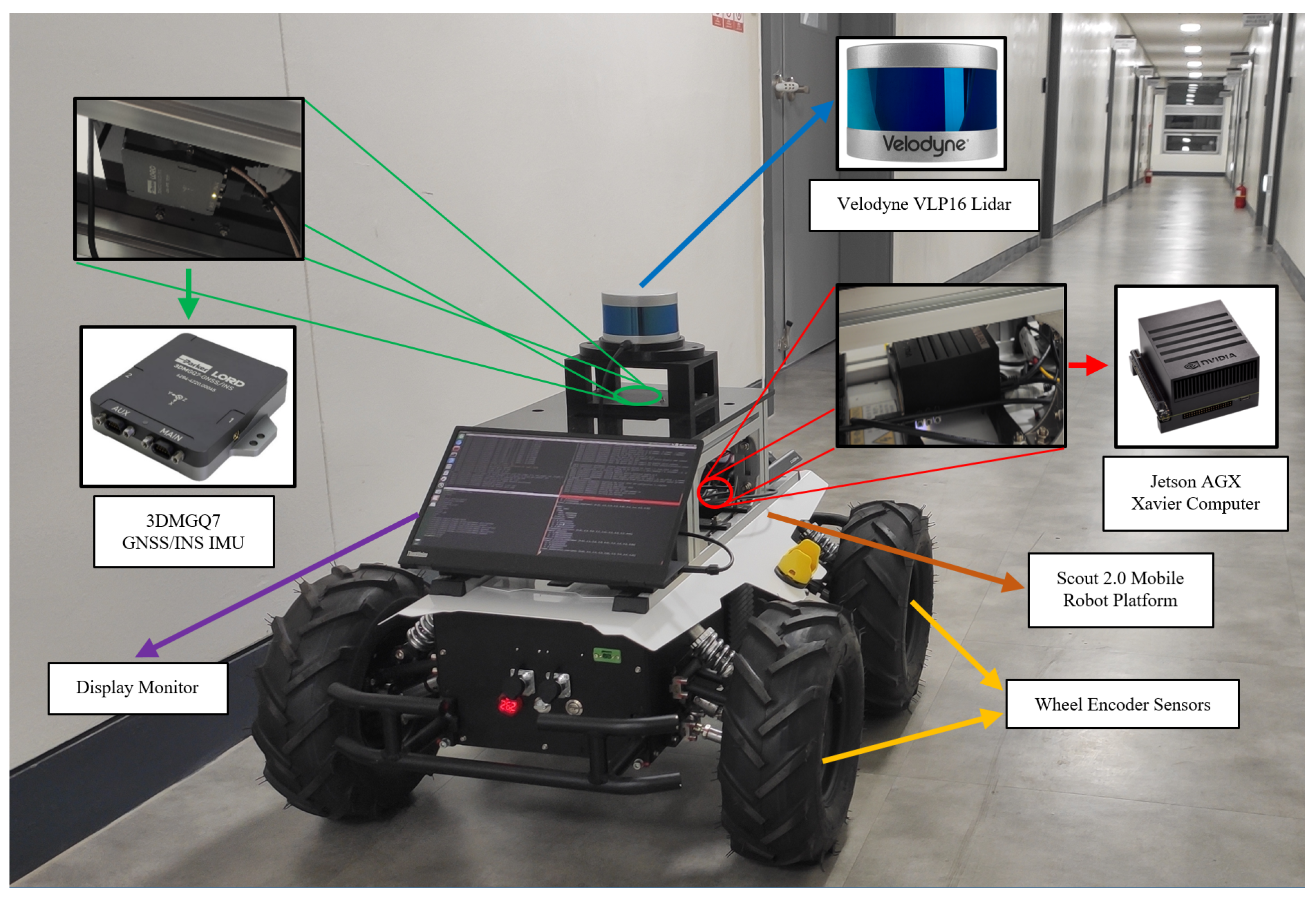
4.1. Experiment Setup
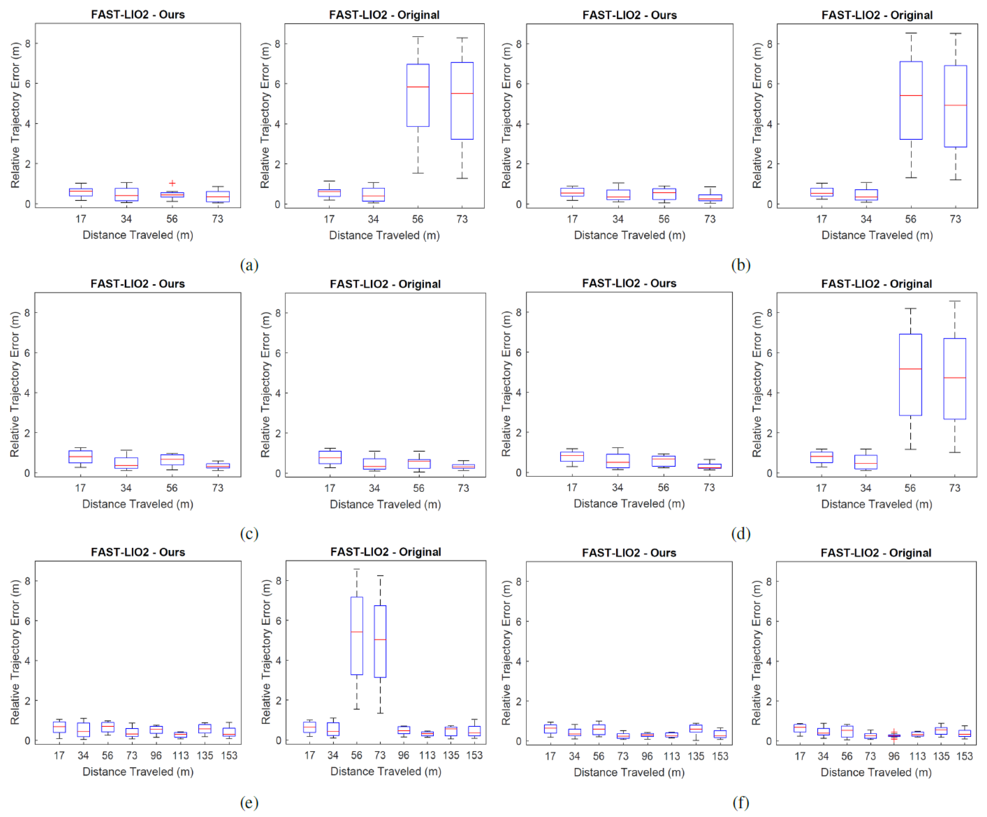
4.2. Error Metrics
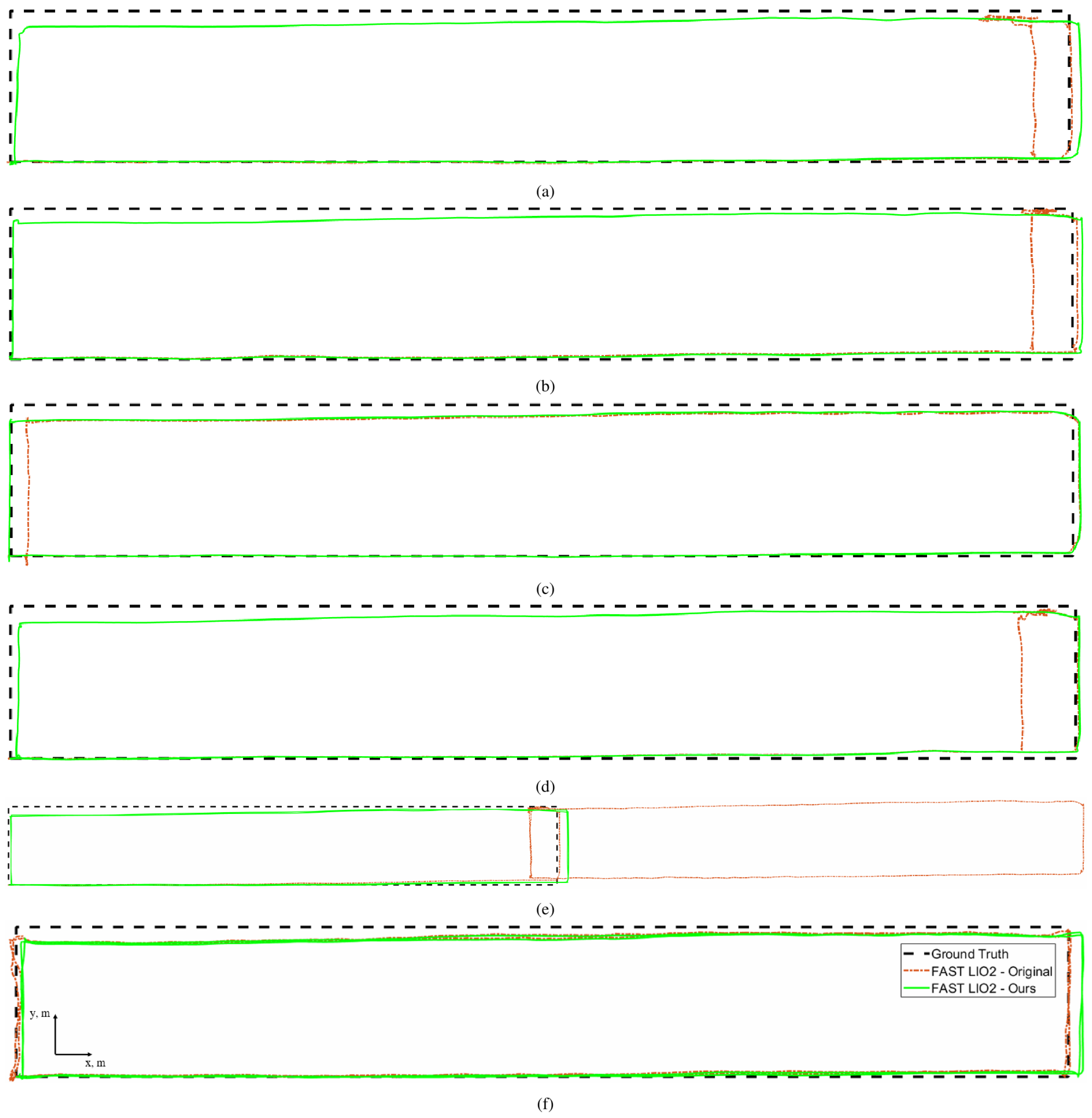
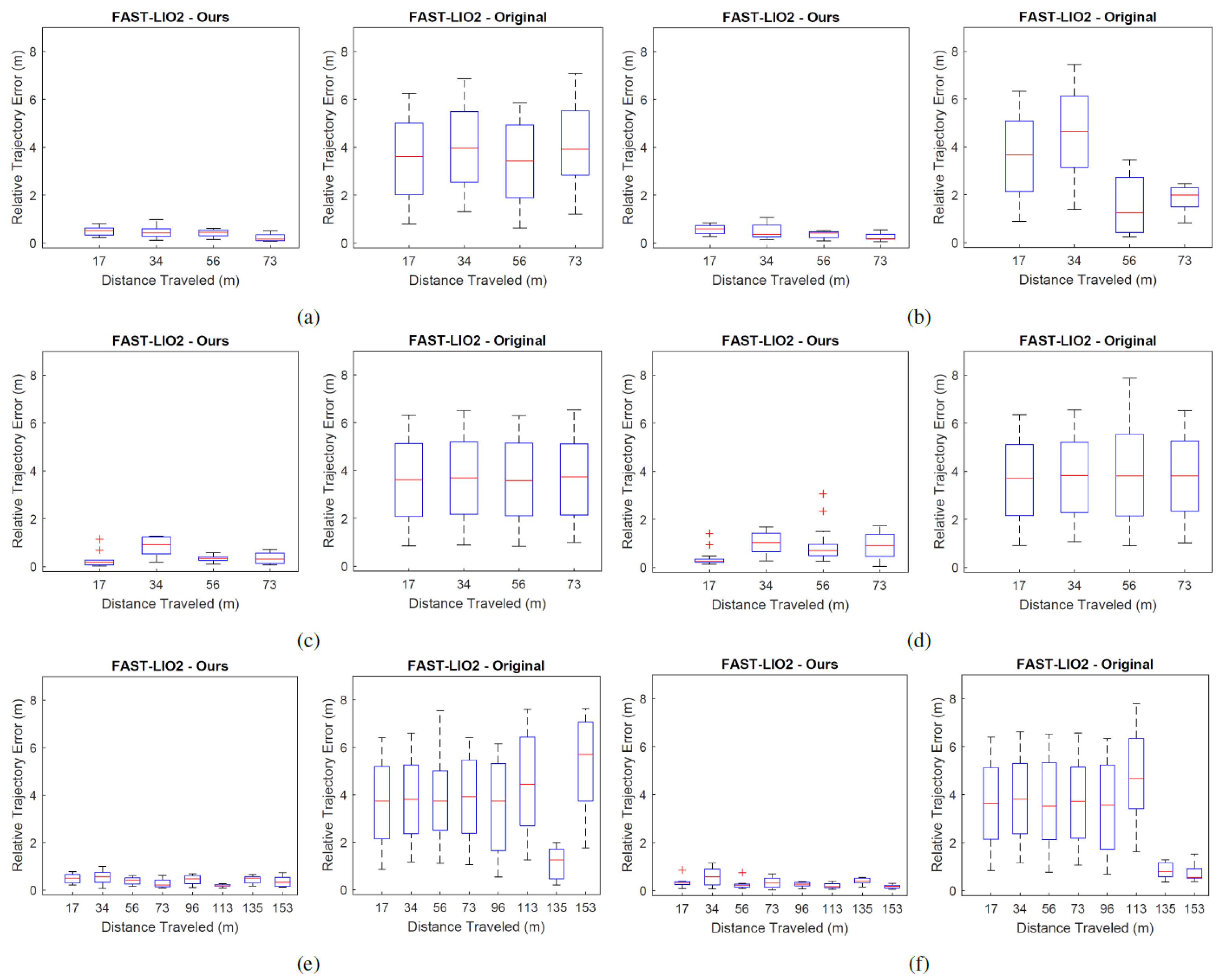
4.3. Flat Section Results
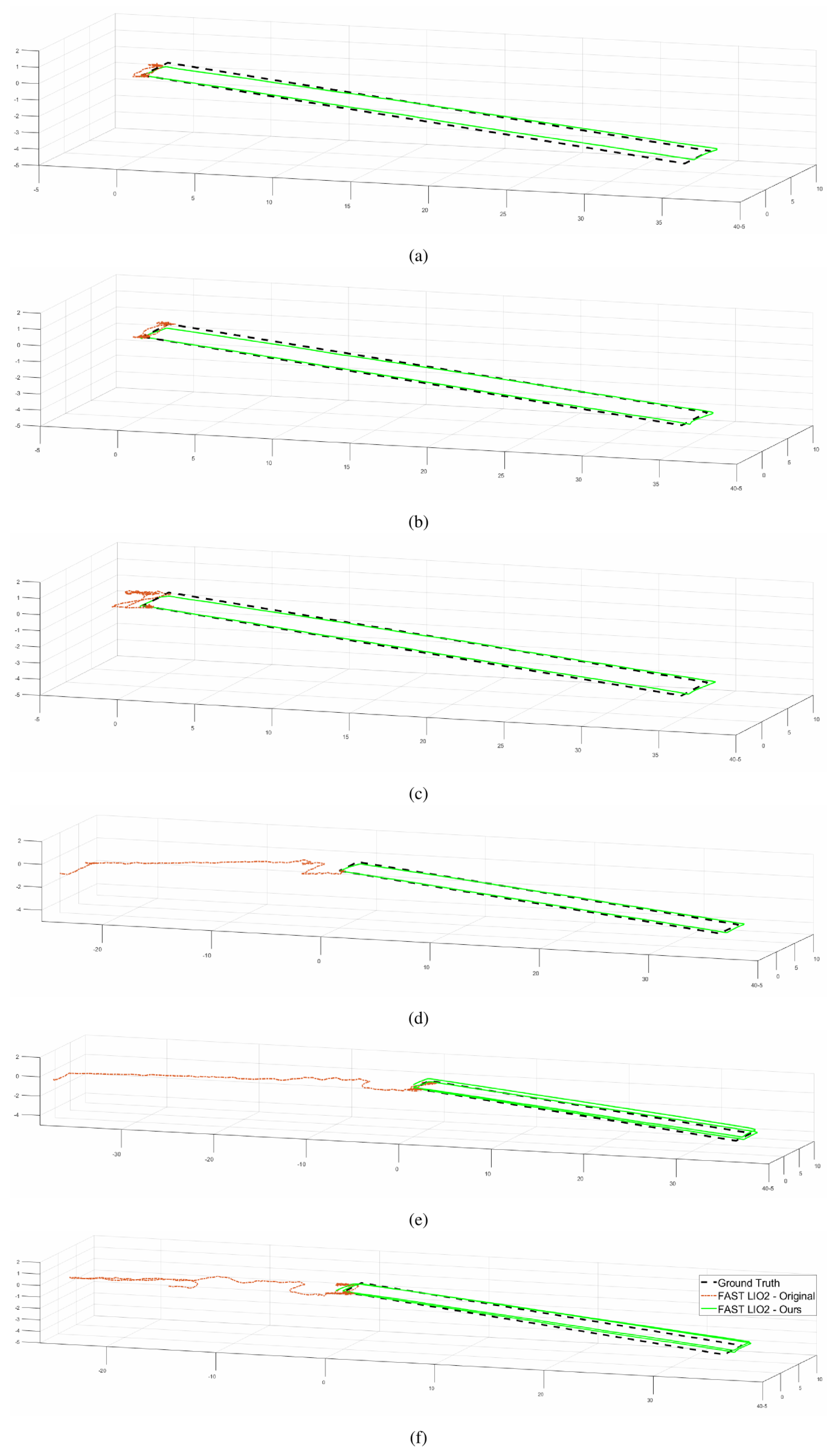
4.4. Inclined Section Results
5. Discussion
6. Conclusions
Author Contributions
Funding
Data Availability Statement
Conflicts of Interest
References
- Jang, H.; Kim, T.Y.; Lee, Y.C.; Song, Y.H.; Choi, H.R. Autonomous Navigation of In-Pipe Inspection Robot Using Contact Sensor Modules. IEEE/ASME Trans. Mechatron. 2022, 27, 4665–4674. [Google Scholar] [CrossRef]
- Sahbel, A.; Abbas, A.; Sattar, T. System Design and Implementation of Wall Climbing Robot for Wind Turbine Blade Inspection. In Proceedings of the 2019 International Conference on Innovative Trends in Computer Engineering (ITCE), Aswan, Egypt, 2–4 February 2019; pp. 242–247. [Google Scholar] [CrossRef]
- Yang, L.; Li, B.; Li, W.; Brand, H.; Jiang, B.; Xiao, J. Concrete defects inspection and 3D mapping using CityFlyer quadrotor robot. IEEE/CAA J. Autom. Sin. 2020, 7, 991–1002. [Google Scholar] [CrossRef]
- Campos, C.; Elvira, R.; Gomez, J.J.; Montiel, J.M.M.; Tardos, J.D. ORB-SLAM3: An Accurate Open-Source Library for Visual, Visual-Inertial and Multi-Map SLAM. IEEE Trans. Robot. 2021, 37, 1874–1890. [Google Scholar] [CrossRef]
- Ferrera, M.; Eudes, A.; Moras, J.; Sanfourche, M.; Le Besnerais, G. OV2SLAM: A Fully Online and Versatile Visual SLAM for Real-Time Applications. IEEE Robot. Autom. Lett. 2021, 6, 1399–1406. [Google Scholar] [CrossRef]
- Jiang, J.; Chen, X.; Dai, W.; Gao, Z.; Zhang, Y. Thermal-Inertial SLAM for the Environments With Challenging Illumination. IEEE Robot. Autom. Lett. 2022, 7, 8767–8774. [Google Scholar] [CrossRef]
- Piao, J.C.; Kim, S.D. Real-Time Visual-Inertial SLAM Based on Adaptive Keyframe Selection for Mobile AR Applications. IEEE Trans. Multimed. 2019, 21, 2827–2836. [Google Scholar] [CrossRef]
- Zhang, J.; Singh, S. LOAM: Lidar Odometry and Mapping in real-time. In Proceedings of the Robotics: Science and Systems Conference (RSS), Berkeley, CA, USA, 12–16 July 2014; pp. 109–111. [Google Scholar]
- Shan, T.; Englot, B. LeGO-LOAM: Lightweight and Ground-Optimized Lidar Odometry and Mapping on Variable Terrain. In Proceedings of the IEEE/RSJ International Conference on Intelligent Robots and Systems (IROS), Madrid, Spain, 1–5 October 2018; pp. 4758–4765. [Google Scholar]
- Shan, T.; Englot, B.; Meyers, D.; Wang, W.; Ratti, C.; Daniela, R. LIO-SAM: Tightly-coupled Lidar Inertial Odometry via Smoothing and Mapping. In Proceedings of the IEEE/RSJ International Conference on Intelligent Robots and Systems (IROS), Las Vegas, NV, USA, 24 October 2020–24 January 2021; pp. 5135–5142. [Google Scholar]
- Wang, H.; Wang, C.; Chen, C.; Xie, L. F-LOAM: Fast LiDAR Odometry and Mapping. In Proceedings of the 2021 IEEE/RSJ International Conference on Intelligent Robots and Systems (IROS), Prague, Czech Republic, 27 September–1 October 2021. [Google Scholar]
- Koide, K.; Miura, J.; Menegatti, E. A portable three-dimensional LIDAR-based system for long-term and wide-area people behavior measurement. Int. J. Adv. Robot. Syst. 2019, 16, 1729881419841532. [Google Scholar] [CrossRef]
- Xu, W.; Cai, Y.; He, D.; Lin, J.; Zhang, F. FAST-LIO2: Fast Direct LiDAR-inertial Odometry. arXiv 2021, arXiv:2107.06829. [Google Scholar] [CrossRef]
- Magnusson, M.; Lilienthal, A.; Duckett, T. Scan Registration for Autonomous Mining Vehicles Using 3D-NDT. J. Field Robot. 2007, 24, 803–827. [Google Scholar] [CrossRef] [Green Version]
- Besl, P.; McKay, N.D. A method for registration of 3-D shapes. IEEE Trans. Pattern Anal. Mach. Intell. 1992, 14, 239–256. [Google Scholar] [CrossRef] [Green Version]
- Cai, Y.; Xu, W.; Zhang, F. ikd-Tree: An Incremental KD Tree for Robotic Applications. arXiv 2021, arXiv:2102.10808. [Google Scholar]
- Akpınar, B. Performance of Different SLAM Algorithms for Indoor and Outdoor Mapping Applications. Appl. Syst. Innov. 2021, 4, 101. [Google Scholar] [CrossRef]
- Filipenko, M.; Afanasyev, I. Comparison of Various SLAM Systems for Mobile Robot in an Indoor Environment. In Proceedings of the 2018 International Conference on Intelligent Systems (IS), Funchal, Portugal, 25–27 September 2018; pp. 400–407. [Google Scholar] [CrossRef]
- Filip, I.; Pyo, J.; Lee, M.; Joe, H. Lidar SLAM Comparison in a Featureless Tunnel Environment. In Proceedings of the 2022 22nd International Conference on Control, Automation and Systems (ICCAS), Jeju, Republic of Korea, 27 November–1 December 2022; pp. 1648–1653. [Google Scholar]
- Kim, G. SC-LeGO-LOAM. 2020. Available online: https://github.com/irapkaist/SC-LeGO-LOAM (accessed on 8 May 2022).
- Kim, G. SC-LIO-SAM. 2021. Available online: https://github.com/gisbi-kim/SC-LIO-SAM (accessed on 5 May 2022).
- Su, Y.; Wang, T.; Shao, S.; Yao, C.; Wang, Z. GR-LOAM: LiDAR-based sensor fusion SLAM for ground robots on complex terrain. Robot. Auton. Syst. 2021, 140, 103759. [Google Scholar] [CrossRef]
- Júnior, G.P.C.; Rezende, A.M.C.; Miranda, V.R.F.; Fernandes, R.; Azpúrua, H.; Neto, A.A.; Pessin, G.; Freitas, G.M. EKF-LOAM: An Adaptive Fusion of LiDAR SLAM With Wheel Odometry and Inertial Data for Confined Spaces With Few Geometric Features. IEEE Trans. Autom. Sci. Eng. 2022, 19, 1458–1471. [Google Scholar] [CrossRef]
- Mandow, A.; Martinez, J.L.; Morales, J.; Blanco, J.L.; Garcia-Cerezo, A.; Gonzalez, J. Experimental kinematics for wheeled skid-steer mobile robots. In Proceedings of the 2007 IEEE/RSJ International Conference on Intelligent Robots and Systems, San Diego, CA, USA, 29 October–2 November 2007; pp. 1222–1227. [Google Scholar] [CrossRef]
- He, D.; Xu, W.; Zhang, F. Kalman Filters on Differentiable Manifolds. arXiv 2021, arXiv:2102.03804. [Google Scholar]
- Zhang, Z.; Scaramuzza, D. A Tutorial on Quantitative Trajectory Evaluation for Visual(-Inertial) Odometry. In Proceedings of the IEEE/RSJ International Conference on Intelligent Robots and Systems (IROS), Madrid, Spain, 1–5 October 2018. [Google Scholar]


| SLAM Algorithm | L1 | L2 | L3 | L4 | L5.1 | L5.2 | L6.1 | L6.2 |
|---|---|---|---|---|---|---|---|---|
| FAST-LIO2 | 11.92 | 12.11 | 1.19 | 12.21 | 11.62 | 23.81 | 1.13 | 0.97 |
| Proposed Method | 1.32 | 1.23 | 1.11 | 1.17 | 1.18 | 0.93 | 1.09 | 1.02 |
| SLAM Algorithm | L1 | L2 | L3 | L4 | L5.1 | L5.2 | L6.1 | L6.2 |
|---|---|---|---|---|---|---|---|---|
| FAST-LIO2 | 12.43 | 15.42 | 11.94 | 11.24 | 12.06 | 19.54 | 11.63 | 17.06 |
| Proposed Method | 1.11 | 1.22 | 1.25 | 1.85 | 1.19 | 1.30 | 1.13 | 1.25 |
Disclaimer/Publisher’s Note: The statements, opinions and data contained in all publications are solely those of the individual author(s) and contributor(s) and not of MDPI and/or the editor(s). MDPI and/or the editor(s) disclaim responsibility for any injury to people or property resulting from any ideas, methods, instructions or products referred to in the content. |
© 2023 by the authors. Licensee MDPI, Basel, Switzerland. This article is an open access article distributed under the terms and conditions of the Creative Commons Attribution (CC BY) license (https://creativecommons.org/licenses/by/4.0/).
Share and Cite
Filip, I.; Pyo, J.; Lee, M.; Joe, H. LiDAR SLAM with a Wheel Encoder in a Featureless Tunnel Environment. Electronics 2023, 12, 1002. https://doi.org/10.3390/electronics12041002
Filip I, Pyo J, Lee M, Joe H. LiDAR SLAM with a Wheel Encoder in a Featureless Tunnel Environment. Electronics. 2023; 12(4):1002. https://doi.org/10.3390/electronics12041002
Chicago/Turabian StyleFilip, Iulian, Juhyun Pyo, Meungsuk Lee, and Hangil Joe. 2023. "LiDAR SLAM with a Wheel Encoder in a Featureless Tunnel Environment" Electronics 12, no. 4: 1002. https://doi.org/10.3390/electronics12041002