Promoting Adversarial Transferability via Dual-Sampling Variance Aggregation and Feature Heterogeneity Attacks

Abstract

At present, deep neural networks have been widely used in various fields, but their vulnerability requires attention. The adversarial attack aims to mislead the model by generating imperceptible perturbations on the source model, and although white-box attacks have achieved good success rates, existing adversarial samples exhibit weak migration in the black-box case, especially on some adversarially trained defense models. Previous work for gradient-based optimization either optimizes the image before iteration or optimizes the gradient during iteration, so it results in the generated adversarial samples overfitting the source model and exhibiting poor mobility to the adversarially trained model. To solve these problems, we propose the dual-sample variance aggregation with feature heterogeneity attack; our method is optimized before and during iterations to produce adversarial samples with better transferability. In addition, our method can be integrated with various input transformations. A large amount of experimental data demonstrate the effectiveness of the proposed method, which improves the attack success rate by 5.9% for the normally trained model and 11.5% for the adversarially trained model compared with the current state-of-the-art migration-enhancing attack methods.

1. Introduction

Deep neural networks (DNN) are currently performing well in computer vision, particularly in the areas of semantic segmentation [1,2,3], instance segmentation [4], target detection [5,6,7], image classification [8,9,10], and other fields. However, the neural network is easily affected by the adversarial sample in the field of computer vision. Adding some interference to the original sample that is difficult for human eyes to detect will make the model output incorrect classification results. Due to the existence of adversarial samples, security issues in such fields as face recognition [11,12], artificial intelligence [13,14,15], and driverless cars [16,17,18], have to be paid attention to [19,20]. In addition, improving the transferability of adversarial samples is to find the weaknesses of the model and thus improve the robustness of the model. In order to better find the flaws in the model, this forces us to design adversarial samples with better attack performance.

In recent years, many methods for generating adversarial samples have been proposed, such as the fast gradient symbolic method [21], iteration-based gradient symbolic method [22], momentum-based iteration [23], and accelerated gradient iteration method [24]. They both showed good attack performance in white box settings. However, it has been demonstrated that the generated adversarial samples are somewhat transferable, which also suggests that adversarial samples made on the source model may be somewhat aggressive towards other models. Because of this transferability nature, an attacker can attack a target model without needing to know any specifics about it, which poses a number of security issues in real life.

The process of improving the transferability of adversarial samples is regarded as the process of improving model generalization [24]. However, methods to improve model generalization usually use better optimization methods or data augmentation. At present, the proposed optimization methods are usually divided into two categories. One is to optimize before each iteration. For example, Lin et al. [24] introduces the Nesterov acceleration gradient to jump out of the local optimal solution before each iteration, so as to obtain a better solution. Wang et al. [25] achieves the same by additional accumulation of the average gradient of the data points sampled on the gradient direction of the previous iteration in order to stabilize the update direction and remove the poor local maximum. The other is to optimize in each iteration process. For example, Dong et al. [23] optimizes by integrating the momentum term into the iterative process. Wang et al. [26] used the gradient variance information of the previous iteration to optimize the current gradient information, so as to achieve the updating direction of the stable gradient.

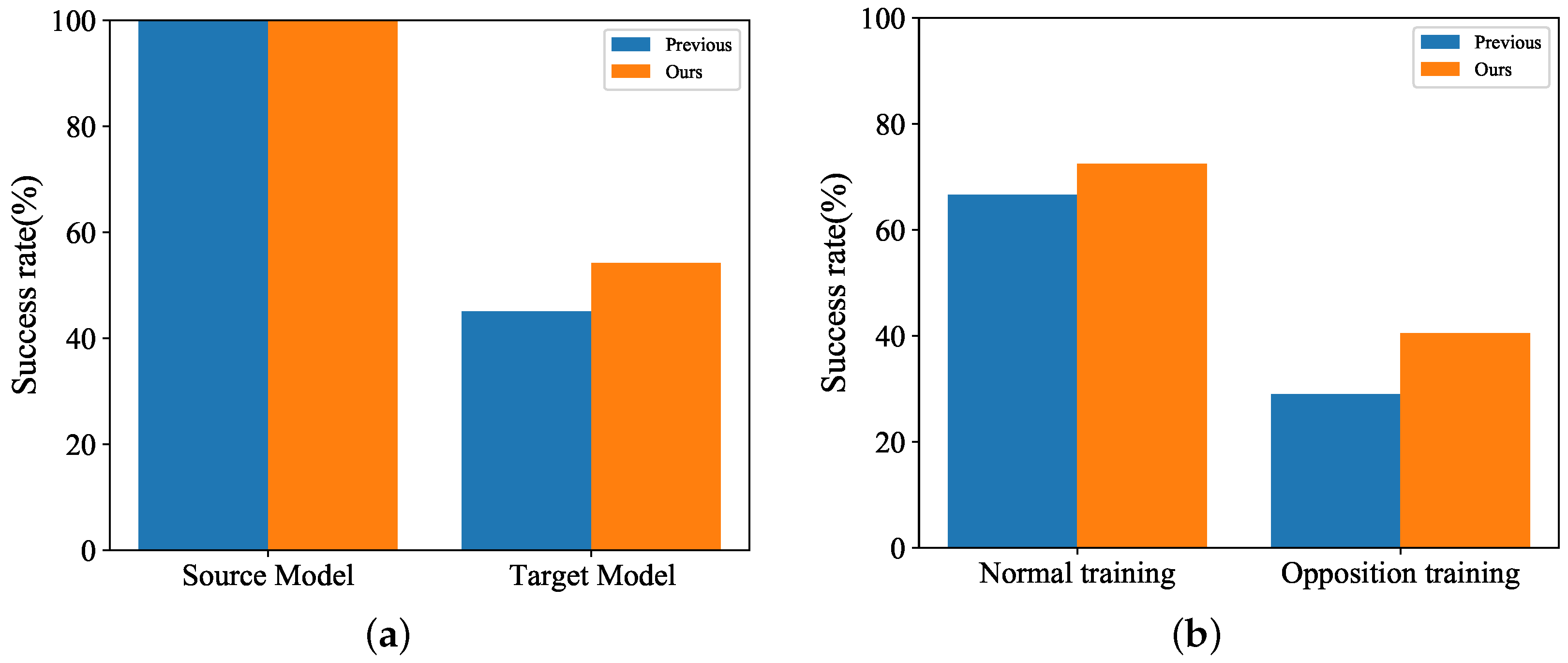
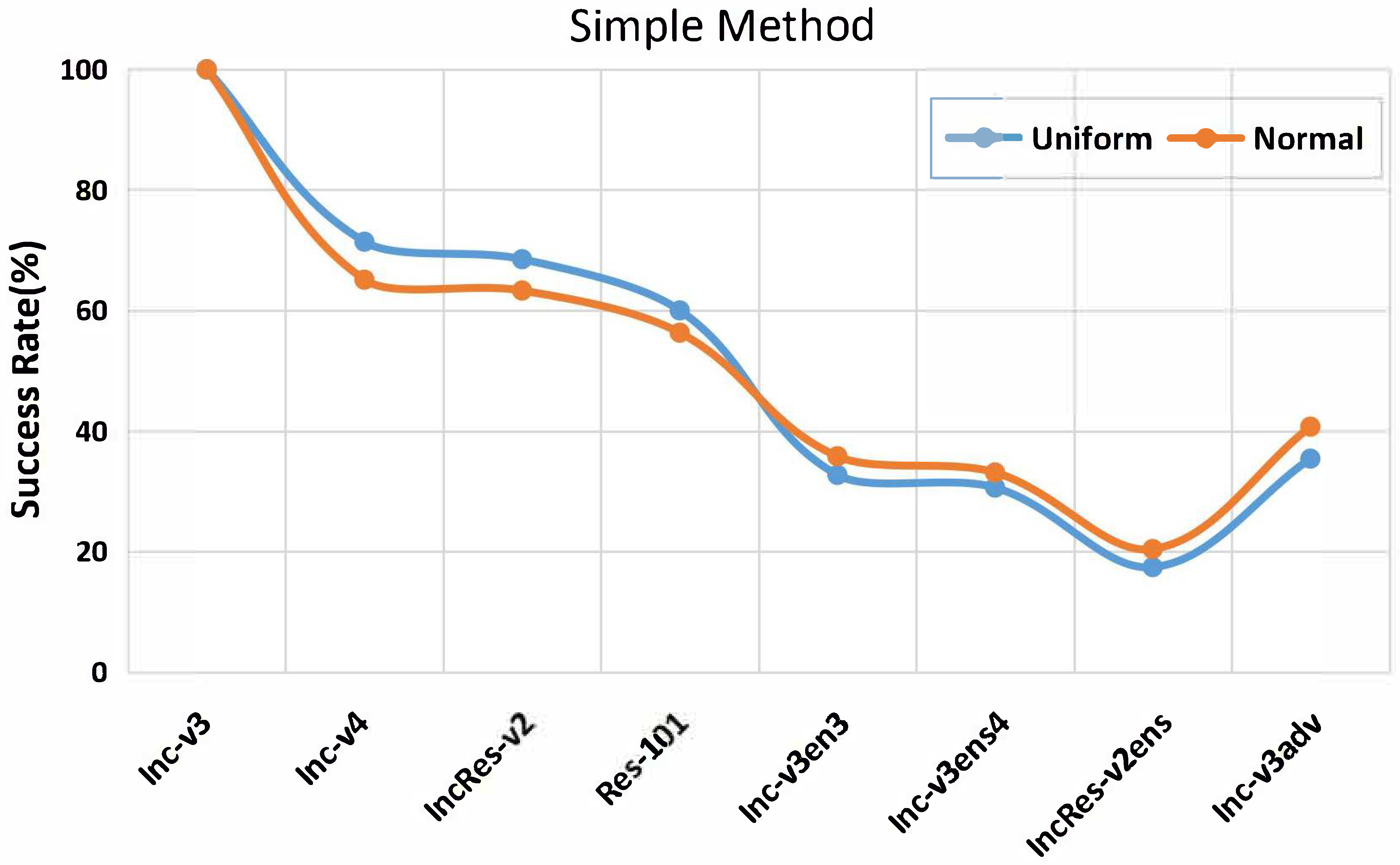
Specifically, these methods are optimized before and after iteration to improve transferability; however, there are still two deficiencies: Although the optimization method, before each iteration, can enhance the portability of opposing samples, this method is prone to overfitting the source model. The reason is that the gradient information added to the original sample each time contains the gradient information of the last iteration. On the one hand, although the gradient is optimized each time in the iterative process to enhance transferability, the adversarial samples produced by this method have weak attack performance against the adversarial training model. The reason is that the process of gradient optimization ignores many characteristic differences between the adversarial sample and the clean image learned by the adversarial training model. In particular, the uniform sampling approach in [26] for finding the gradient variance information has high transferability for the normally trained model, but shows poor transferability for the adversarially trained model, as shown in Figure 1. This has encouraged us to create a more effective method for discovering model flaws in order to increase transferability and address some of the issues that arise in the aforementioned two classes of approaches.

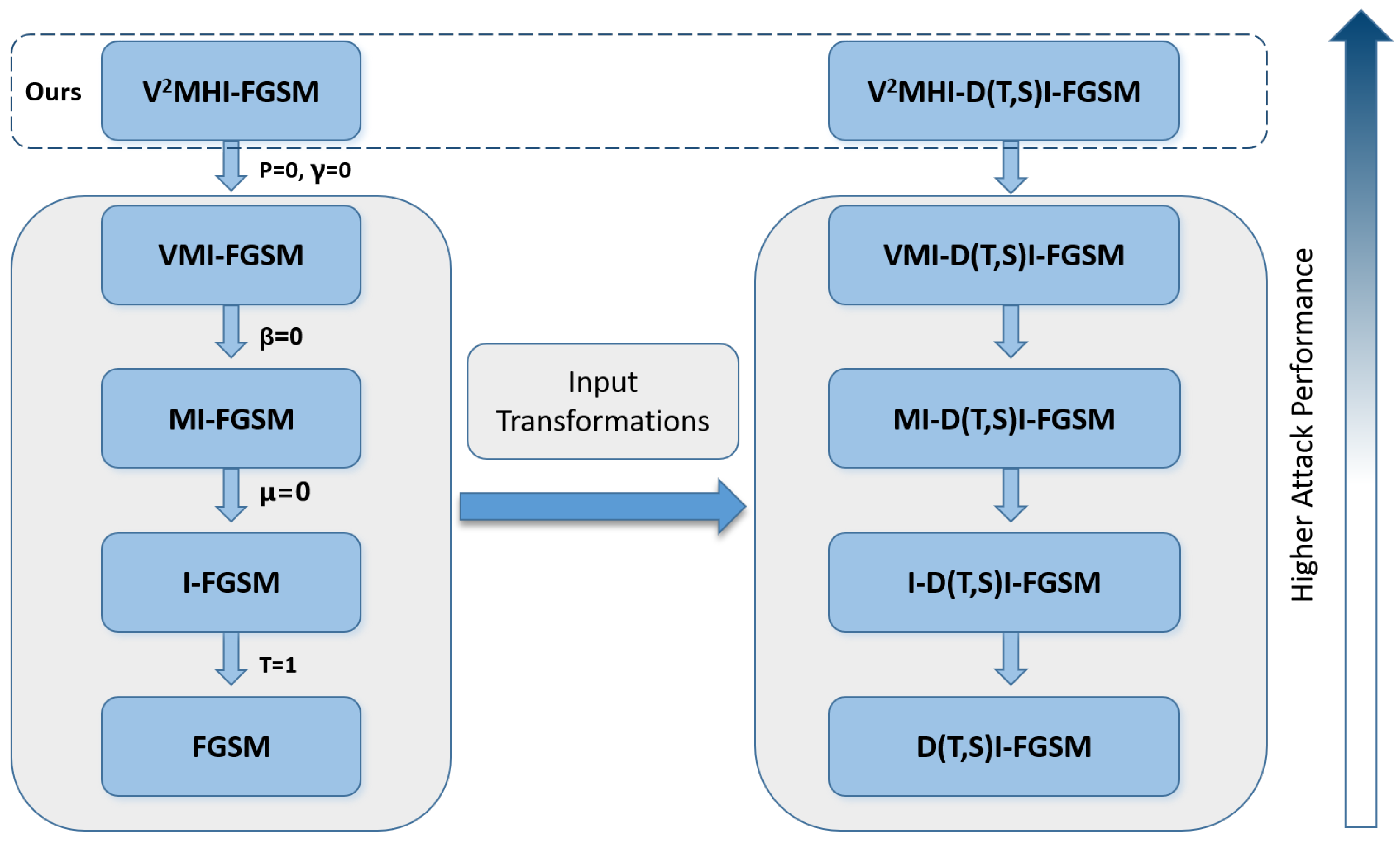
In this study, we propose a Dual-Sampling Variance Aggregation and Feature Heterogeneity Attacks (V${}^2$MHI-FGSM), which reduces the overfitting of the adversarial samples to the source model by destroying the model-specific feature information, especially the black-box model with adversarial training, which has a better attack success rate.

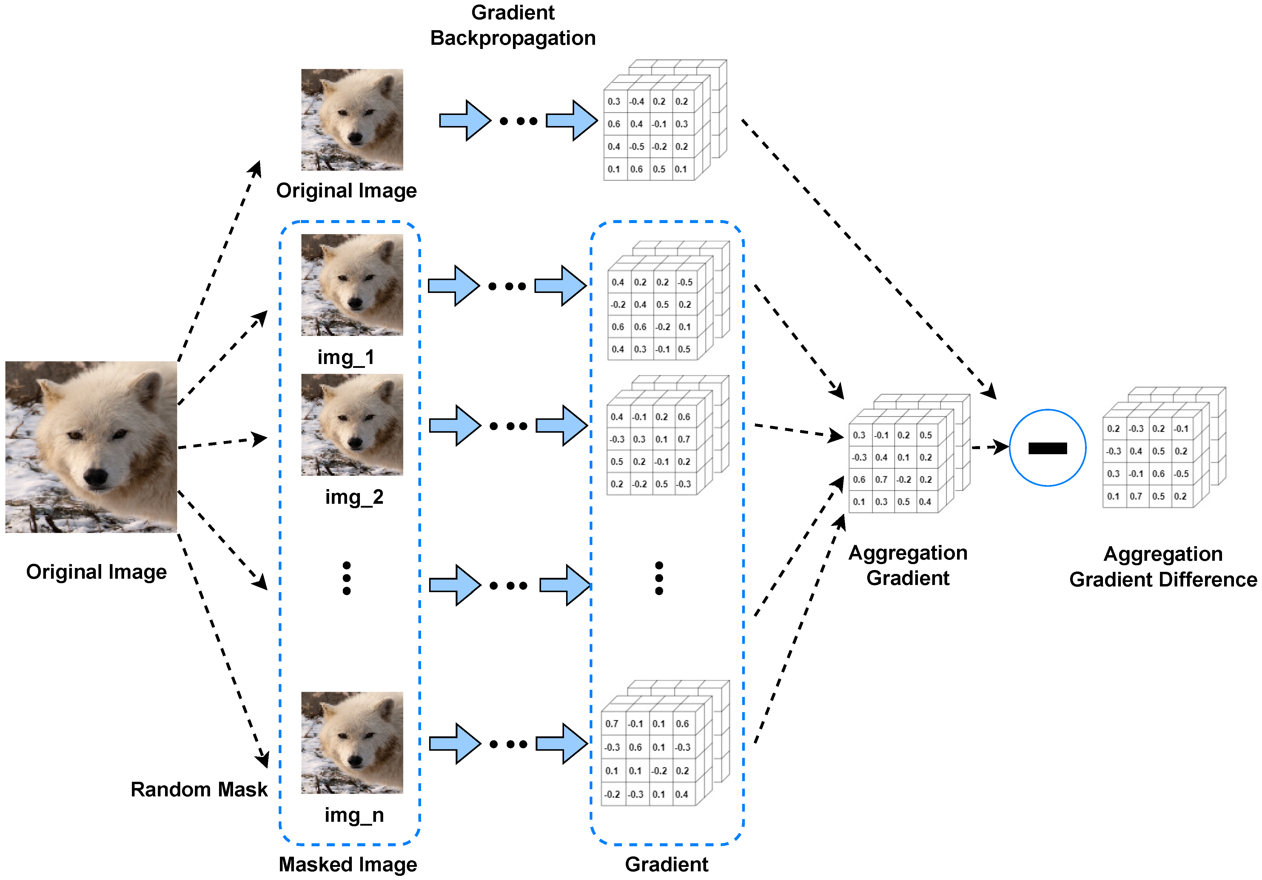
Our method is as follows: we add the aggregate gradient difference to the original image to make the original image achieve feature heterogeneity, so as to solve the overfitting of the source model by the adversarial samples. More specifically, the original image is preprocessed by randomly deleting pixels due to the specific differences between the image of the deleted pixel and the original image in the network; therefore, we add this difference to the original sample, which is usually called feature heterogeneity. Further, in order to enhance the black-box attack success rate of adversarial samples against the adversarial training model with high robustness, we aggregate the variance information obtained from uniform distribution and normal distribution sampling. More specifically, we average the gradient variance information obtained by the two sampling methods, which will effectively improve the attack success rate of adversarial samples on the more robust model. Additionally, the adversarial samples generated by our method perform better in the standard training model. Finally, our method has been improved through both the pre-iteration and iteration processes, and the experiment shows that it is superior in the context of a black box.

Our main contributions are summarized as follows:

• The adversarial examples generated by the existing methods have weak generalization and low transferability, which is due to an overfitting to the source model. In order to direct the creation of more transferable adversarial examples, we introduce aggregated gradient differences.
• At the same time, the adversarial samples produced by the current state-of-the-art methods show poor transferability to the adversarially trained classification model. On this basis, we introduce the dual-sampling variance aggregation method to further improve the transferability of the adversarial samples on the adversarially trained model.
• Numerous tests on various classification models show that the adversarial examples produced by our suggested method have better transferability than cutting-edge adversarial attack techniques.

2. Related Work

Given a clean sample x as the input, f as the classifier, y as the true label of x, $f(x,\theta )$ is the output after x is input to the model, which is the predicted label of x, and $\theta$ is the network parameter. We denote $J(x,y,\theta )$ as the loss function of the classifier f, which generally defaults to the cross-entropy loss function. We define adversarial attack as finding an imperceptible adversarial example $x^{adv}$ to mislead the model $f(x^{adv};\theta )\ne y$, and the adversarial example satisfies $\left|\right|x^{adv}-x{\left|\right|}_p\le ϵ$ this constraint, where $\left|\right|·{\left|\right|}_p$ denotes the p-norm distance, and we keep p = ∞ in line with previous work.

2.1. Adversarial Attacks

Existing adversarial attacks can roughly be divided into two settings based on the threat of adversarial examples to the model: (a) In a white-box attack, the attacker has total access to all of the model’s hyperparameters, outputs, gradients, model architecture, etc. (b) In a black-box attack, the attacker only has access to the model’s output; all of the other parameters are unknown. The current white-box attack research has produced good attack performance, and while researching the white-box attack, it is discovered that the adversarial samples produced on one model exhibit good transferability between different models. The use of adversarial examples, also known as “black-box attacks”, can deceive both the source model and other models simultaneously. To address the low portability of current adversarial attack methods, several improved adversarial (gradient-based) attack methods have been put forth. Dong et al. [23] suggested incorporating momentum into iterative gradient-based attacks from gradient optimization. To further improve the migrability, Lin et al. [24] proposed the accelerated gradients of Nestorve from image optimization. According to Liu et al. [24], the migrability can be increased even more by combining the aforementioned gradient-based optimization and image-based optimization techniques with integrated model attacks that target multiple models. Therefore, our method can be used in conjunction with both integrated model attacks to produce more migrable adversarial samples.

Additionally, according to some studies, applying different input transformations to the original image can enhance the transferability of adversarial examples even more. For example, DIM [27] randomly crops and fills the input image within a certain range with a fixed probability, and inputs the processed image into the model to generate noise to enhance transferability. The translation-invariant [28] uses a set of images to compute gradients. Dong et al. [28] shift the image by a small amount to reduce the computation of gradients, and then they approximate the gradient by convolution the gradient of the unshifted image with the kernel matrix. Scale-invariant methods [24] compute gradients by scaling the input image to a set of images by a factor of 1/$2^i$ (i denotes a hyperparameter) to enhance the mobility of the generated adversarial examples. Meanwhile, current work integrates input transformation-based attacks, ensemble model attacks, and gradient-based attack techniques to further enhance the transferability of adversarial examples. Our approach is a novel gradient-based assault that not only relies on gradients but also on picture features to produce more portable adversarial examples. It may be integrated with ensemble model attacks and input transformation-based approaches to increase portability.

2.2. Adversarial Defense

Finding the weaknesses in adversarial attacks is crucial for improving the robustness of deep learning models. However, one of the most effective methods to strengthen the model is adversarial training, which involves including adversarial samples in the training set. Numerous studies have demonstrated that this technique can successfully increase the model’s robustness [29]. Ensemble adversarial training, which combines adversarial training with the ensemble model, is an alternative to applying it to a single model. The method has been shown to be resistant to adversarial samples with migration when the adversarial training is combined with the integrated model to create integrated adversarial training, which trains the adversarial samples produced by the integrated model alongside clean samples.

Based on the above methods to enhance robustness, recent studies have proposed some variants to enhance the robustness of the model. Xie et al. [30] used random resizing and padding (R&P) at image input to mitigate the effect of adversarial perturbations. Liao et al. [31] cleaned the images by using a trained high-level representation denoiser (HGD) on the images to enhance the recognition. Xu et al. [21] proposed to detect adversarial samples by compressing the extracted features using bit-depth reduction (bit-Red). A JPEG-based defensive compression framework called feature distillation (FD) [32] can successfully target adversarial samples. An end-to-end image compression model that can successfully fend off hostile samples is called ComDefend [33]. Stochastic smoothing (RS) was used by Cohen et al. [34] to train a trustworthy ImageNet classifier. An automatically derived supervised neural representation purifier (NRP) based model that can successfully purify adversarially perturbed images was created by Naseer et al. [35].

3. Methodology

In this section, we first provide a brief overview of previous gradient-based attack methods. The feature heterogeneity attack (VMHI-FGSM) and the dual-sampling variance aggregation attack(V${}^2$MI-FGSM) are then described in detail. Finally, the difference between our method V${}^2$MHI-FGSM method and previous methods is introduced.

3.1. Gradient-Based Adversarial Attack Methods

This section mainly introduces typical adversarial attack algorithms based on gradient improvement.

Fast Gradient Sign Method (FGSM). FGSM [36] generates adversarial examples with one-step update:

$$x^{adv}=x+ϵ·sign\left({\nabla }_{x}J(x,y,\theta )\right),$$

(1)

where ${\nabla }_x$ is the gradient of the loss function J(·) with respect to x. In general, J(·) is the cross-entropy loss function, and sign(·) represents the function of finding the sign of the gradient.

Iterative Fast Gradient Sign Method (I-FGSM). I-FGSM [22] extends the one-step attack on FGSM to multiple steps by introducing a step size $\alpha$:

$$x_{t+1}^{adv}=x_t^{adv}+\alpha ·sign\left({\nabla }_{x_t^{adv}}J(x,y,\theta )\right),$$

(2)

where $x_1^{adv}=x$, $\alpha =ϵ/T$ is a small step size, and T is the number of iterations.

Momentum Iterative Fast Gradient Sign Method (MI-FGSM). MI-FGSM [23] accumulates the gradient of each iteration of I-FGSM as momentum into the next iteration to improve mobility:

$$g_{t+1}=u·g_t+\frac{{\nabla }_{x_t^{adv}}J(x_t^{adv},y;\theta )}{\left|\right|{\nabla }_{x_t^{adv}}J(x_t^{adv},y;\theta ){\left|\right|}_1},$$

(3)

$$x_{t+1}^{adv}=x_t^{adv}+\alpha ·sign\left(g_{t+1}\right),$$

where $g_t$ is the gradient of the t-th iteration with $g_0$ = 0 and $\mu$ is the decay factor.

Nesterov Iterative Fast Gradient Sign Method (NI-FGSM). NI-FGSM [24] introduces the idea of Nesterov [37] gradient descent, replacing $x_t^{adv}$ in Equation (3) with $x_t^{adv}+\alpha ·\mu ·g_t$ to further improve the transferability of MI-FGSM.

Variance momentum Iterative Fast Gradient Sign Method (VMI-FGSM). VMI-FGSM [26] uses the gradient variance information of the previous iteration to adjust the current gradient information, so as to better stabilize the gradient update direction. It replace Equation (3) by

$$g_{t+1}=u·g_t+\frac{{\nabla }_{x_t^{adv}}J(x_t^{adv},y;\theta )+v_t}{\left|\right|{\nabla }_{x_t^{adv}}J(x_t^{adv},y;\theta )+v_t{\left|\right|}_1},$$

(4)

where $v_{t+1}=\frac{1}{N}{\sum }_{i=1}^N{\nabla }_{x}J(x_i,y)-{\nabla }_{x}J(x_t^{adv},y)$, $x_i$ is a sample randomly sampled from a certain uniform distribution range of x.

3.2. Feature Heterogeneity Attack

In order to eliminate the local optimum and achieve higher transferability than I-FGSM [22], MI-FGSM [23], which is based on gradient optimization, stabilizes the update direction of the current gradient by adding the gradient from the previous iteration. On this basis, the method based on image optimization NI-FGSM [24] performs an operation similar to preprocessing before the image is input into the model. It introduces Nesterov’s idea to accelerate the gradient to have a look-ahead feature before each image enters the model. The present image input model may thus converge more quickly and attain higher transferability. However, because the gradient information from the previous iteration is added to the image during each iteration phase, this will result in the phenomena of overfitting to the source model. Due to the adversarial samples’ final addition of too much source model feature information after several iterations, the adversarial samples ends up being overfitted.

To reduce the overfitting phenomenon after multiple iterations of the adversarial sample, we suggest Feature Heterogeneity Guided Momentum Iterative (HMI-FGSM), an NI-FGSM version that shares many of the same properties as NI-FGSM—the same forward-looking features as FGSM. More specifically, we add some different features to the image of each iteration. The HMI-FGSM, as illustrated in Figure 2, finds the difference between the averaged gradient and the gradient of the original image after averaging the gradient obtained after the image has had random pixel points removed. This discrepancy exists between the original image and the image with the erased pixels, and finally introduces the difference into the original image. The updating process can be summarized as follows:

$${\widehat{x}}_t^{adv}=x_t^{adv}+\alpha ·D_{t-1},$$

(5)

$${\widehat{g}}_t={\nabla }_{{\widehat{x}}_t^{adv}}{J}_f({\widehat{x}}_t^{adv},y),$$

(6)

$$g_t=\mu ·g_{t-1}+\frac{{\widehat{g}}_t}{\left|\right|{\widehat{g}}_t{\left|\right|}_1},$$

(7)

$$x_{t+1}^{adv}=x_t^{adv}+\alpha ·sign\left(g_t\right),$$

(8)

$$D_t=\frac{1}{N}\sum _{i=1}^N{\nabla }_{{\widehat{x}}_t^{adv}\odot M_P^m}-{\widehat{g}}_t,M_p\sim Bernoulli(1-p)$$

(9)

where $M_P$ represents a binary matrix of the same size as x, and ⊙ represents element-wise multiplication. The ensemble number N represents the random mask number for the input x, and $D_{t-1}$ represents the feature difference from the previous iteration. For forward guiding, HMI-FGSM takes into account the gradient difference around the input x rather than all past gradients as in NI-FGSM, which can enhance adversarial attacks.

3.3. Dual-Sampling Variance Aggregation Attack

In the current research on the latest gradient-based attack methods, in order to stabilize the gradient update direction and significantly increase the transferability of adversarial examples, the work VMI-FGSM [26] technique adjusts the current gradient information using the gradient variance data from the previous iteration based on MI-FGSM [23]. When determining the gradient variance information from the previous iteration, VMI-FGSM uses the uniformly distributed sampled samples and then determines the discrepancy between it and the initial sample gradient. We discover that the adversarial sample attack performance obtained through uniform sampling performs better on a model that has been normally trained but worse on one that has been trained in an adversarial manner, as shown in Figure 3.

We examine the attack performance of the adversarial samples with a focus on the stronger models because they are now more frequently used. As a result, we were motivated to create an adversarial sample that performs better in attacks on both normally trained and adversarially trained models.

Based on some problems existing in the above methods, we use dual-sampling variance aggregation to further optimize the gradient in the iterative process of each gradient optimization. The gradient variance information is averaged to replace the original single-layer sampling. We compute the variance aggregated gradient for the t-th iteration as follows:

$$V\left(x_t^{adv}\right)=\frac{V_t^U+V_t^N}{2}$$

(10)

$$V\left(x\right)=\frac{1}{N}\sum _{i=1}^N{\nabla }_{x^i}J(x_i,y)-{\nabla }_{x}J(x_t^{adv},y)$$

(11)

where $x^i=x+r_i$. When the sampling method is normal $r_i\sim$ N [0, ${(\gamma ·ϵ)}^d$]; when the sampling method is uniform $r_i\sim$ U [−${(\beta ·ϵ)}^d$, ${(\beta ·ϵ)}^d$], and N [0, $a^d$] and U [$b^d$, $c^d$] represent the d-dimensional normal distribution and uniform distribution, respectively.

After computing the double-sampled variance aggregation gradient, we can use the double-sampled aggregation gradient variance at the (t − 1)-th iteration to adjust the gradient of $x_t^{adv}$ at the t-th iteration to stabilize the gradient. Finally, we fuse feature heterogeneity attack and double sampling variance aggregation attack to obtain our final method V${}^2$MHI-FGSM, as shown in Algorithm 1. Overall, our method not only shows better performance, but our method can be integrated with DIM, TIM, and SIM to achieve better results.

Algorithm 1 Dual-Sampling Variance Aggregation and Feature Heterogeneity Attacks

Input:  A clean samples x and ground truth labels y, and a classifier f with parameters $\theta$ and loss function J; the magnitude of perturbation value $ϵ$; number of iterations T and decay factors $\mu$; the factor $\beta$ for the upper bound of neighborhood and number of example N for variance tuning; the upper limit factor $\gamma$ for the variance field and for the sampling number $N_{nor}$; the image pixel deletion number P and gradients aggregation number $N_{agg}$. Output:  Adversarial samples $x^{adv}$ 1: $\alpha =ϵ/T$ 2: $g_0=0;D_0=0;v_0=0;x_0^{adv}$ = x 3: for  $t=0\to T-1$do 4:  ${\widehat{x}}_t^{adv}=x_t^{adv}+\alpha ·D_{t-1}$ 5:  Calculate the gradient ${\widehat{g}}_t={\nabla }_{{\widehat{x}}_t^{adv}}J({\widehat{x}}_t^{adv},y;\theta )$ 6:  Updating $g_{t+1}$ by momentum-based variance aggregation and feature differences $$g_{t+1}=\mu ·g_t+\frac{{\widehat{g}}_t+v_t^2}{\left|\right|{\widehat{g}}_t+v_t^2{\left|\right|}_1}$$ (12) 7:  Update $D_t$ by Equation (9) 8:  Update $v_{t+1}^2=V\left(x_t^{adv}\right)$ by Equation (10) 9:  Update $x_{t+1}^{adv}$ by applying the sign of gradient $$x_{t+1}^{adv}=x_t^{adv}+\alpha ·sign\left(g_{t+1}\right)$$ (13) 10: end for 11: $x^{adv}=x_T^{adv}$ 12: return$x^{adv}$

3.4. Relationships among Various Attacks

Here, we provide a summary of the connections between numerous adversarial assaults from the FGSM to the present, as shown in Figure 4. Our method V${}^2$MHI-FGSM degrades to VMI-FGSM if the upper limit factor $\gamma =0$ and the integration number $N_{agg}$ = 0. If the upper limit factor $\beta$ in VMI-FGSM is set to 0, then VMI-FGSM are degraded to MI-FGSM. If the decay factor $\mu$ = 0, then both MI-FGSM are degraded to I-FGSM. If the number of iterations T = 1 in I-FGSM, then it is degraded to FGSM. Meanwhile, the above adversarial attack method can be combined with various input transformations (i.e., DIM, TIM, and SIM) to form a more powerful counterattack method.

4. Experiments

To validate the attack performance of our proposed V${}^2$MHI-FGSM attack method, we performed extensive experimental validation on the standard ImageNet2012 dataset [38]. We set up the data, models, etc., needed for the experiments, and then our method was also compared with the baseline in the case of integration with several input transformations. Note that the attack success rates in this article are all the false-recognition rates of the model. Our method clearly outperforms the baseline attack success rate, as shown in

Table 1. Attack success rates (%) of adversarial attacks against the eight baseline models under single-model setting. The adversarial examples are crafted on Inc-v3. * indicates the white-box model.

Attack	Inc-v3 *	Inc-v4	IncRes-v2	Res-101	Inc-v3_ens3	Inc-v3_ens4	IncRes-v2_ens	Inc-v3_adv	Average
FGSM	67.3	25.7	26.0	24.5	10.2	10.4	4.5	12.1	22.5
I-FGSM	100.0	20.3	18.5	16.1	4.6	5.2	2.5	6.4	21.7
MI-FGSM	100.0	45.6	42.3	35.8	14.1	12.4	6.2	19.3	34.4
NI-FGSM	100.0	51.5	49.4	40.6	13.0	12.3	6.8	20.0	36.7
VMI-FGSM	100.0	71.4	68.5	60.0	32.7	30.6	17.4	35.4	52.0
VNI-FGSM	100.0	76.8	75.0	64.6	34.5	33.3	19.2	40.0	55.0
V${}^{\mathbf{2}}$MI-FGSM	99.9	70.4	68.0	62.3	39.4	38.8	23.9	42.5	55.6
V${}^{\mathbf{2}}$MHI-FGSM	99.8	76.2	73.9	67.6	44.8	42.5	26.4	48.5	60.0

. Finally, we further investigated the discard probability P and the set number N of feature differences in gradient aggregation, as well as the hyperparameters $\gamma$ and N in orthogonal sampling.

4.1. Experimental Setup

Data. Similar to [26], we randomly selected 1000 images of different categories from the ILSVRC2012 validation set, and we also make sure that all these 1000 images can be correctly classified by each model in this paper; randomly selected, these images are pre-resized to 299 × 299 × 3.

Model. Our model has four normally trained models Inception-v3(Inc-v3) [39], Inception-v4(Inc-v4), Inception-Resnet-v2(IncRes-v2) [40], Resnet-v2-101(Res-101) [41], and four adversarially trained models, namely ens3-adv-Inception-v3(Inc-v3${}_{ens3}$), ens4-Inception-v3(Inc-v3${}_{ens4}$), ens-adv-Inception-ResNet-v2(IncRes-v2${}_{ens}$), and adv-Inception-v3(Inc-v3${}_{adv}$) [42].

Baseline. Four gradient-based attack techniques—the MI-FGSM, NI-FGSM, VMI-FGSM, and VNI-FGSM—are compared to our approach. We also combined our method with various input transforms, namely DIM, TIM, SIM, and DTS (which represents the integration of the three of them), denoted as V${}^2$M(N)HI-DTS, V${}^2$MHI-FGSM-DIM, V${}^2$MHI-FGSM-TIM, and V${}^2$MHI-FGSM-SIM. Finally, our method was integrated into the attack method of the ensemble model [24] to further demonstrate the effectiveness of our method.

Hyper-parameters. We are consistent with the parameter settings in [26]: the maximum perturbation is $ϵ$ = 16, step size $\alpha$ = 1.6, the number of iterations T = 10, $\beta$ = 3/2, N = 20 in uniform sampling. For the momentum term, we set the decay factor u=1 to the same as [23,24]. For DIM, the transformation probability is set to 0.5. For TIM, we use a Gaussian kernel with a kernel size of 7 × 7. For SIM, the number of scale replicas is 5 (i.e., i = 0, 1, 2, 3, 4). In our proposed method V${}^2$MHI-FGSM, the drop probability when attacking the normal training model is P = 0.2, the set in the aggregated gradient is N${}_{agg}$ = 10. For the parameter $\gamma$ in sampling the positive distribution, it is set to 3/2, the domain the number of samples within N${}_{nor}$ = 20.

4.2. Comparison with Gradient-Based Attacks

We first generate adversarial examples in the single-model setting and test its attack performance on both white-box and black-box, as shown in Table 1. Next, we generate adversarial examples in the ensemble model setting and test their attack performance on the ensemble model, as shown in

Table 2. Success rates (%) against eight models in a multi-model setup through various gradient-based iterative attacks. Adversarial examples are generated by integrating on four models, namely Inc-v3, Inc-v4, IncRes-v2, and Res-101. * indicates the white-box model.

Attack	Inc-v3 *	Inc-v4 *	IncRes-v2 *	Res-101 *	Inc-v3_ens3	Inc-v3_ens4	IncRes-v2_ens	Inc-v3_adv
FGSM	64.8	49.3	43.9	68.8	15.8	15.1	8.9	15.5
I-FGSM	99.9	98.6	95.6	99.8	19.1	16.8	10.4	18.1
MI-FGSM	99.9	98.7	95.0	99.9	39.7	35.5	23.8	36.4
NI-FGSM	100.0	99.8	99.2	99.9	41.2	34.9	22.9	37.1
VMI-FGSM	100.0	99.6	99.3	99.9	77.2	73.0	59.9	75.1
VNI-FGSM	100.0	99.9	99.9	99.9	78.7	73.9	59.9	77.9
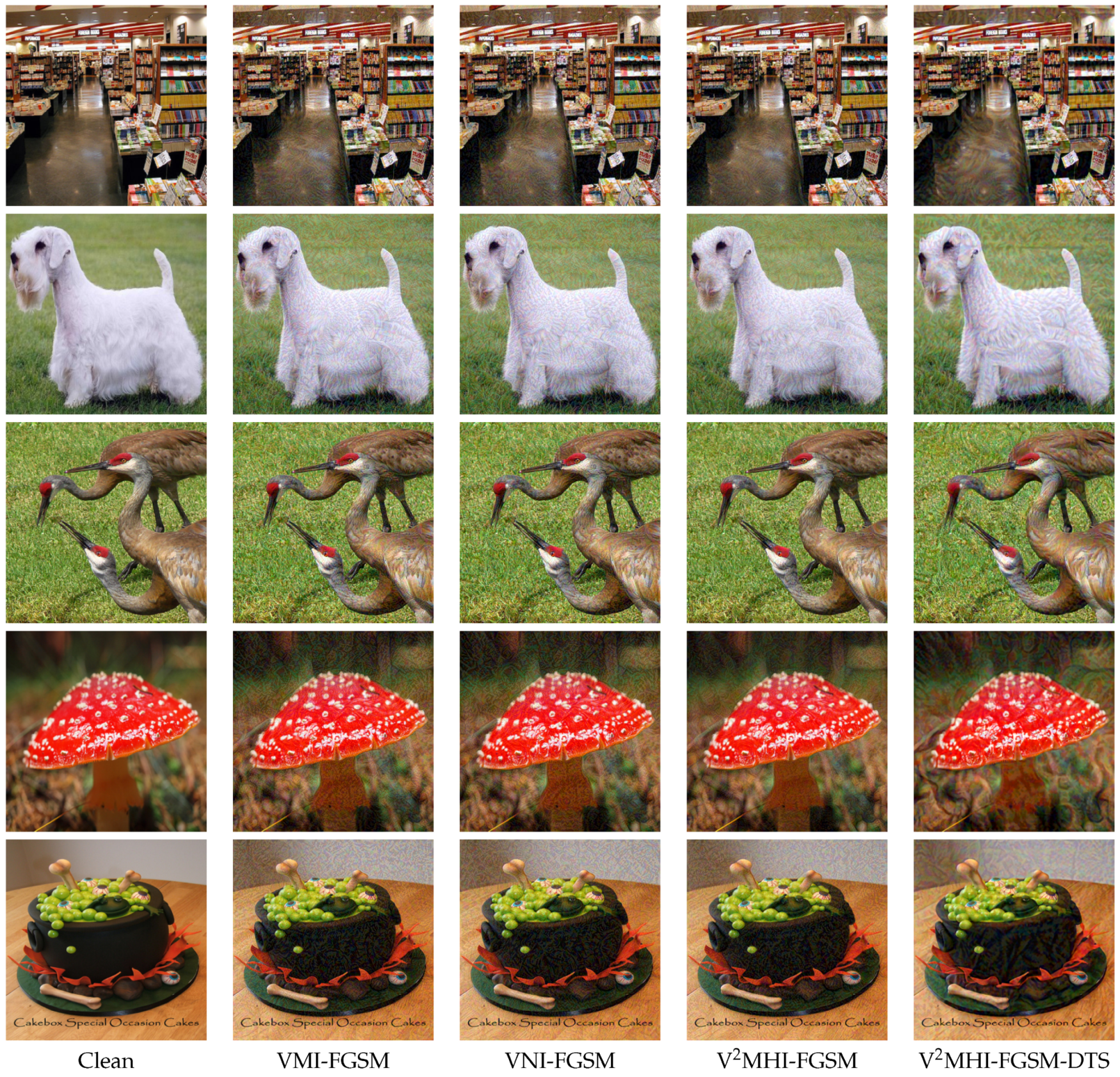
V${}^{\mathbf{2}}$MHI-FGSM	99.8	99.5	98.5	99.4	79.4	77.2	66.5	78.0

. Finally, we randomly select five clean images and visualize the adversarial samples produced after four adversarial attacks, as shown in Figure 5.

Attack a single model. We first produced adversarial samples using six adversarial attack methods on a single model, and the produced adversarial samples were attacked against the baseline methods in this paper; these adversarial attack methods include FGSM, I-FGSM, MI-FGSM, NI-FGSM, VMI-FGSM, and our proposed dual-sampling variance aggregation with feature heterogeneity attacks V${}^2$MHI-FGSM and V${}^2$MI-FGSM. All of the above attack algorithms produced adversarial samples on the Inc-v3 model, and the generated adversarial samples were tested on Inc-v3 and the remaining seven models, i.e., the misclassification rate of the adversarial samples on the corresponding models.

Our method shows the best block attack performance among the existing methods, as shown in Table 1. Meanwhile, our method and the optimal method were compared with four different models as source models, respectively, as shown in

Table 3. The success rates (%) on eight models in the single model setting by various gradient-based iterative attacks. The adversarial examples are crafted on Inc-v3, Inc-v4, IncRes-v2, and Res-101, respectively. * indicates the white-box model.

Model	Attack	Inc-v3	Inc-v4	IncRes-v2	Res-101	Inc-v3_ens3	Inc-v3_ens4	IncRes-v2_ens	Inc-v3_adv
Inc-v3	VMI-FGSM	100.0 *	71.4	68.5	60.0	32.7	30.6	17.4	35.4
	V${}^2$MHI-FGSM	99.7*	75.7	73.8	67.1	43.4	40.6	25.0	46.0
Inc-v4	VMI-FGSM	78.1	99.7 *	70.5	63.0	38.5	36.6	24.1	35.2
	V${}^2$MHI-FGSM	79.9	97.5 *	75.0	66.7	48.2	46.5	32.5	45.3
IncRes-v2	VMI-FGSM	77.9	72.3	97.8*	68.0	47.6	40.0	34.8	44.1
	V${}^2$MHI-FGSM	76.3	71.0	94.2 *	67.9	53.1	47.4	44.7	49.7
Res-101	VMI-FGSM	75.7	68.4	69.9	99.3 *	44.6	40.9	29.9	42.9
	V${}^2$MHI-FGSM	79.4	75.2	74.3	99.7 *	54.0	52.4	40.4	53.0

.

Attack ensemble model. Lin et al. [24] showed that the adversarial samples produced by integrating logits from multiple models have better transferability. There are three types of ensemble methods for general models, namely ensemble in loss function, ensemble in prediction result, and ensemble in logits. In this paper, we fuse the logits output of the four models. In this section, our ensemble attack method averages the logit outputs of the models Inception-v3, Inception-v4, Inception-Resnet-v2, and Inception-v2-101; our approach also exhibits optimal attack performance, as shown in Table 2.

4.3. Input Transformation Attack

To further enhance the migrability of the generated adversarial samples, we combine previous gradient-based attack techniques with three input transformations (e.g., DIM [27], TIM [28], and SIM [24]). Additionally, we combine our suggested method with these three input transformations, as shown in

Table 4. These adversarial samples are made on single models, * indicates the white-box model.

Attack	Inc-v3 *	Inc-v4	IncRes-v2	Res-101	Inc-v3_ens3	Inc-v3_ens4	IncRes-v2_ens	Inc-v3_adv
DIM	99.1	65.7	62.2	54.9	20.4	18.9	9.8	24.4
V${}^2$MHI-DIM(Ours)	98.3	77.0	74.6	69.4	45.8	44.7	27.8	50.3
TIM	100.0	49.0	44.7	39.5	24.5	20.6	13.7	25.4
V${}^2$MHI-TIM(Ours)	99.5	77.1	74.5	67.6	60.0	59.8	44.7	60.4
SIM	100.0	70.4	66.4	61.9	32.3	32.0	16.5	36.1
V${}^2$MHI-SIM(Ours)	99.8	89.9	88.3	83.5	64.9	62.3	45.2	65.8
DTS	99.3	84.8	80.8	76.6	66.8	62.7	47.0	64.5
V${}^2$MHI-DTS(Ours)	99.2	89.4	88.0	84.4	81.2	78.5	68.5	79.9

, and experimentally show that both our method and earlier adversarial attack methods perform at their best when doing so.

Combining these input transformations with the gradient-based attack algorithm, while integrating the combined results over multiple models, as shown in Table 4, our approach also exhibits optimal performance.

As described in [43], the combination of DIM, TIM, and SIM can be performed as DTS, which can further enhance the portability of the gradient-based attack algorithm. Further, we combined our method with DTS, as shown in Table 4 and

Table 5. These adversarial samples are made on four ensemble models, * indicates the white-box model.

Attack	Inc-v3	Inc-v4	IncRes-v2	Res-101	Inc-v3_ens3	Inc-v3_ens4	IncRes-v2_ens	Inc-v3_adv
DIM	99.4 *	97.4 *	94.7 *	99.8 *	56.3	50.7	36.4	53.1
V${}^2$MHI-DIM(Ours)	99.7 *	99.0 *	98.3 *	98.4 *	82.0	79.8	71.3	82.2
TIM	99.8 *	98.0 *	95.0 *	99.9 *	61.3	56.7	47.8	54.5
V${}^2$MHI-TIM(Ours)	99.7 *	99.4 *	97.8 *	98.6 *	88.0	87.7	83.2	87.3
SIM	99.9 *	99.3 *	98.5 *	100.0 *	78.5	74.4	60.4	74.1
V${}^2$MHI-SIM(Ours)	99.9 *	99.9 *	99.7 *	99.8 *	91.3	90.2	85.9	91.2
DTS	99.6 *	98.9 *	97.9 *	99.7 *	92.1	90.2	86.6	89.8
V${}^2$MHI-DTS(Ours)	99.8 *	99.7 *	99.5 *	99.4 *	95.6	94.5	92.5	95.4

, which shows optimal attack performance for the remaining four models of black-box attacks, especially on the adversarially trained models, indicating that our method generates better generalization of adversarial examples.

4.4. Ablation Experiment on Hyper-Parameters

To better show the performance of the double-sampling variance aggregation and feature heterogeneity attack methods, we conducted ablation experiments on variance parameters and N${}_{nor}$ in the double-sampled variance ensemble. The characteristic heterogeneous attacks in the heterogeneity attack aggregation number N${}_{agg}$ and discard probability P on the performance of the V${}^2$MHI-FGSM method, as well as the parameter settings of uniform sampling, are consistent with [26]. We used Inc-v3 as a source model to make confrontation samples, and set the default settings $\gamma$ = 3/2, N${}_{nor}$ = 20, P = 0.2, and N${}_{agg}$ = 10.

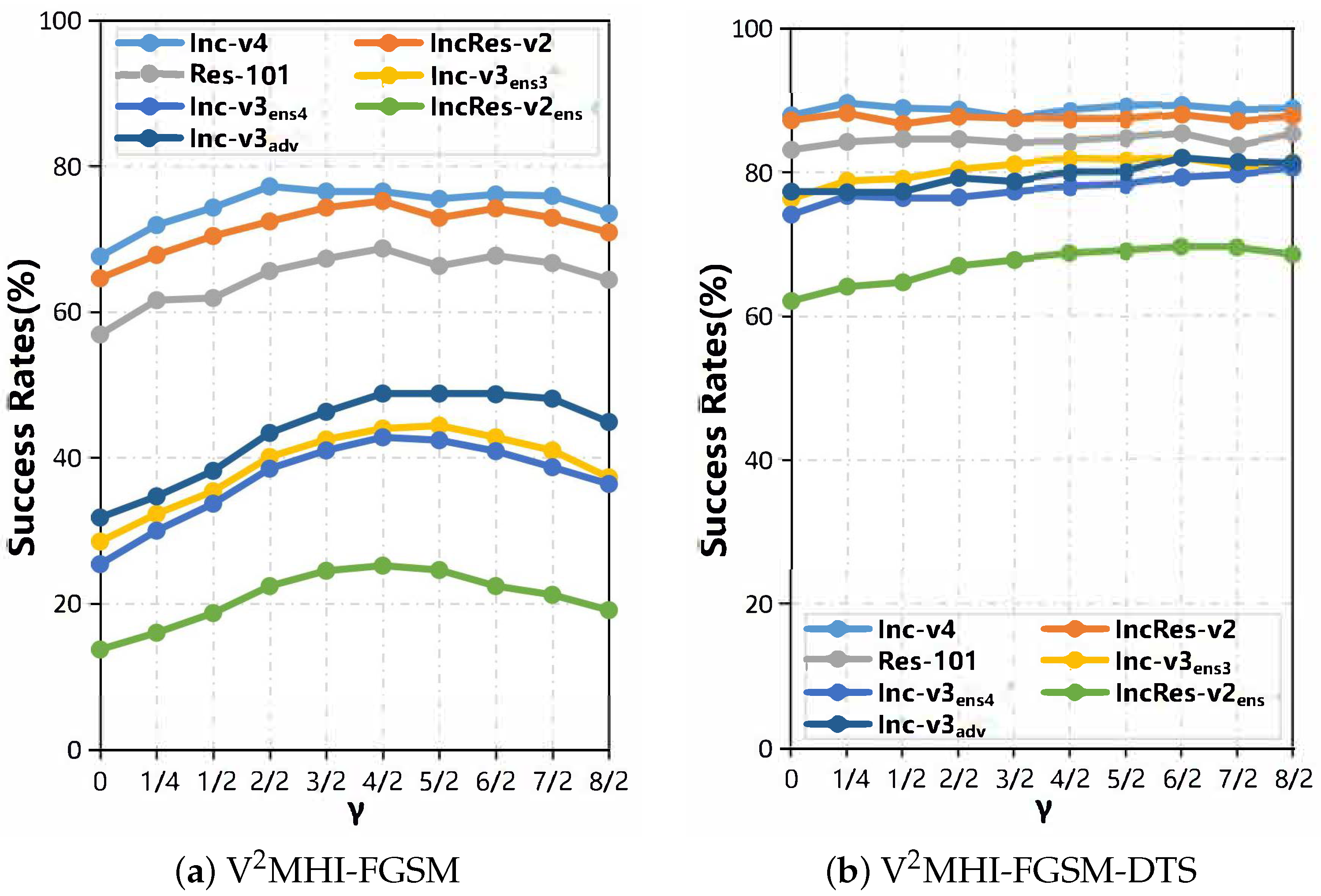
The variance parameter $\gamma$ in normal distribution sampling. We studied the parameter $\gamma$ and determined the impact of the neighborhood size in the neighborhood distribution on the attack success rate of the black-box settings in Figure 6. Fixed N${}_{nor}$ = 20. When $\gamma$ = 0, V${}^2$MI-FGSM degenerates to VMI-FGSM, and the lowest migration is achieved. When $\gamma$ = 1/5, although the samples are very small, our proposed two-sample variance aggregation attack can effectively improve the migration of adversarial samples. With the increase of $\gamma$, when $\gamma$ = 4/2, the average success rate of the black-box attack of our method reaches its peak, especially for the transferability of the combination of training models. As a result, we choose $\gamma$ = 4/2.

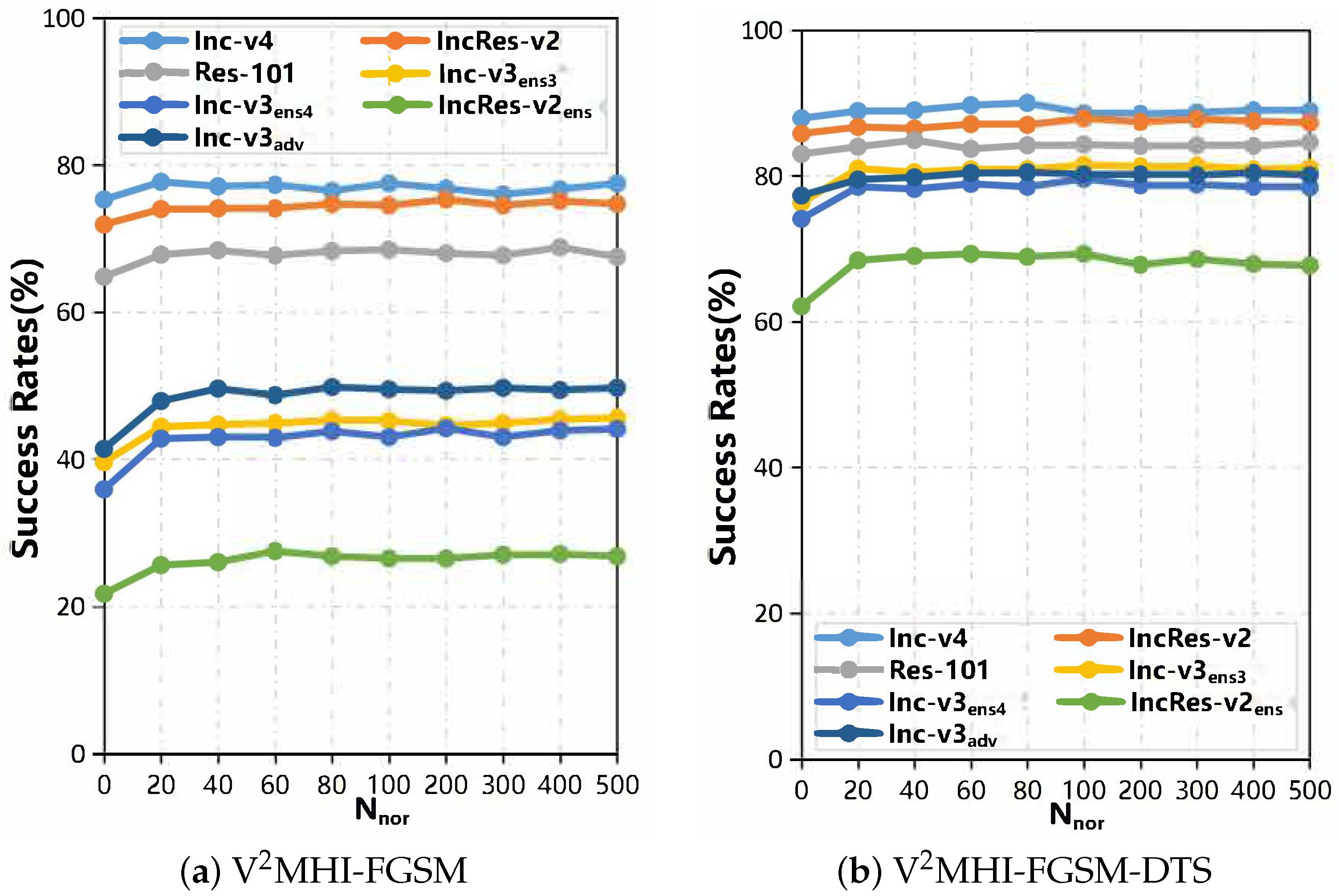
The number of samples in the field N${}_{nor}$. We analyzed the impact of the number of samples in the sample in a normal distribution ($\gamma$ fixed to 4/2). As shown in Figure 7, when N${}_{nor}$ = 0, the V${}^2$MI-FGSM degenerates to VMI-FGSM, and the lowest migration is achieved. When N${}_{nor}$ = 20, the migration of the adversarial samples of our method production is significantly higher. When the N${}_{nor}$ continues to increase, the transferability can increase slowly. Because a large number of gradients need to be calculated at each iteration, the greater the value of N${}_{nor}$, the greater the calculation overhead. In order to balance calculation overhead and migration, we set N${}_{nor}$ = 20 in the experiment.

In short, when N${}_{nor}$ > 20, N${}_{nor}$ has a small impact on migration, and parameter $\gamma$ plays an important role in the impact success rate. In our experiments, the ultra-parameters $\gamma$ and N${}_{nor}$ in the dual sampling square polymerization method were set to 4/2 and 20, respectively.

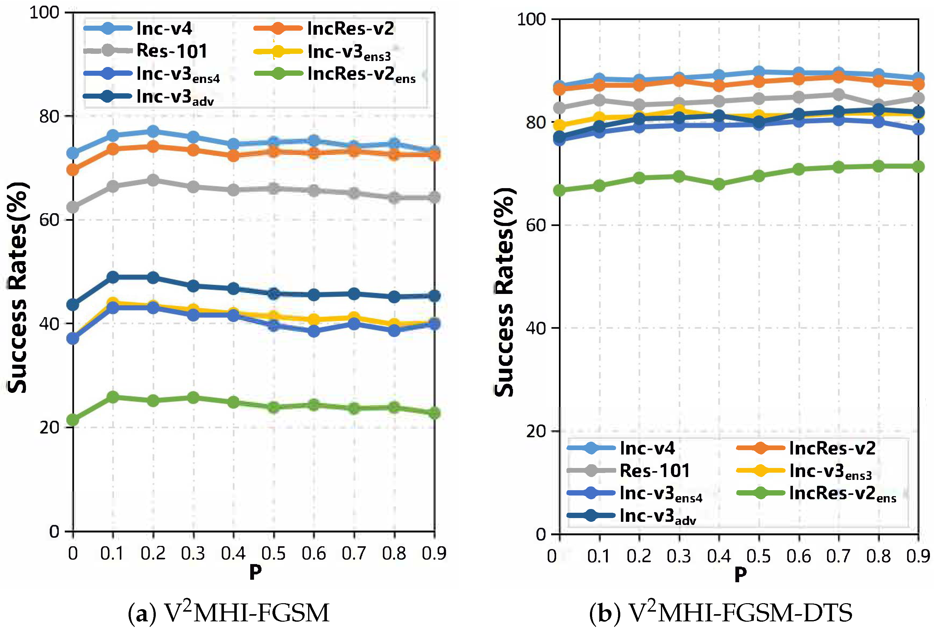
About the number of random deletions of image pixels. In Figure 8, we studied the impact of discarding probability on the success rate of an attack under black-box settings. Among them, fixed N${}_{agg}$ = 10 increased the abandoned probability from 0 to 0.9, and the step length was 0.1. When P = 0, V${}^2$MHI-FGSM degenerates to V${}^2$MI-FGSM, and the lowest migration can be achieved. When P = 0.1, the probability of discarding is very small, but the success rate of the black-box attack has improved significantly. When P > 0.1, the success rate of the black-box attack gradually decreases with the increase of P; therefore, we discard the probability to 0.2, when the average success rate of a black-box attack is maximized.

The number of deleted pixel images N${}_{agg}$. Finally, we analyzed the effects of the aggregate N${}_{agg}$ on the attack success rate under the black-box settings (discard probability P = 0.2). As shown in Figure 9, when N${}_{agg}$ = 0, V${}^2$MHI-FGSM degenerates to V${}^2$MI-FGSM, and the lowest migration is achieved. When N${}_{agg}$ = 1, although the number of aggregation is small, our method can significantly improve the transferability of the adversarial samples. With the increase of N${}_{agg}$ with the step length, the power of black-box attacks only increases in a small amount. Because the process of seeking gradient aggregation requires a lot of computing resources, we balance the success rate of black-box attacks and computing resources. We set up N${}_{agg}$ = 10.

In short, the discarding probability P plays a key role in migration, and when N${}_{agg}$ > 10, N${}_{agg}$ has a small impact. Therefore, in our experiments, we set P to 0.2, N${}_{agg}$ = 10.

5. Conclusions

In this paper, we propose a dual-sample variance aggregation with a feature heterogeneity attack method to improve the transferability of the adversarial samples. Although based on the the previous method, our method has certain differences: our method starts from both pre-iteration and in-iteration perspectives, optimizing the image before the iteration and optimizing the gradient during the iteration, respectively. First, feature information with differences is added to the images, and then the gradients of the images are optimized by double-sampling variance aggregation to improve the transferability of the adversarial samples, as evaluated on the standard ImageNet dataset. Our method maintains similar success rates to the state-of-the-art methods in the white-box setting and significantly improves the transferability of the adversarial samples in the black-box setting.

Our state-of-the-art V${}^2$MHI-FGSM attack method with three input transformations for integration achieves an average attack success rate of more than 83%, and our method with integrated models and three input transformations for combination achieves an average attack success rate of more than 97%, significantly improving the transferability of the adversarial samples. Additionally, on eight different models, our approach outperforms cutting-edge attack methods by an average of 8%. Our research demonstrates that the current defense models are technically flawed, necessitating an increase in the models’ robustness.