Article

Two-Dimensional Positioning with Machine Learning in Virtual and Real Environments

1
Department of Mechatronics and Automation, Faculty of Engineering, University of Szeged, 6720 Szeged, Hungary
2
Ultinous, 1117 Budapest, Hungary
*
Author to whom correspondence should be addressed.
Electronics 2023, 12(3), 671; https://doi.org/10.3390/electronics12030671
Submission received: 30 December 2022 / Revised: 22 January 2023 / Accepted: 26 January 2023 / Published: 29 January 2023

Abstract

:
In this paper, a ball-on-plate control system driven only by a neural network agent is presented. Apart from reinforcement learning, no other control solution or support was applied. The implemented device, driven by two servo motors, learned by itself through thousands of iterations how to keep the ball in the center of the resistive sensor. We compared the real-world performance of agents trained in both a real-world and in a virtual environment. We also examined the efficacy of a virtually pre-trained agent fine-tuned in the real environment. The obtained results were evaluated and compared to see which approach makes a good basis for the implementation of a control task implemented purely with a neural network.

1. Introduction

This work is looking for a solution to transfer artificial intelligence to a physical problem, namely a design and implementation of two-dimensional neural network-controlled positioning. Balancing is one of the biggest challenges in the field of control. There are many models, such as the inverted pendulum, which can be either double or triple, or the ball-rail system, where the ball balances on a rail.
The ball-on-plate system is also a general example in the field of nonlinear control. Since many control methods have been implemented on such systems, this task provides good foundations for the implementation and evaluation of purely artificial intelligence-based controls. The system consists of a ball and a table that can be moved in two dimensions. The ball position can be detected using a camera or some kind of contact-based sensor. Depending on the design, the inclination of the table is usually controlled by two or more motors. These servo motors can be used to tilt the plate along two or more axes. The two-dimensional system can be understood as a combination of two ball-and-beam systems; by tilting the plate, the ball can be moved and positioned on the table. In terms of mechanical design, as Figure 1 shows, the servo motors are usually connected to the table by two arms and cardan joints [1].
In the one design approach, two servo motors are considered as two independent linear kinematic chains, such that the movement of one of the motors may result in a larger displacement than the movement of the other motor [2]. In another approach, the table is grasped like a gyroscope and the separate rings are moved by a servo drive [3].
To observe the ball position, two main approaches can be distinguished: computer-vision-based and resistive sensor-based solutions. In the case of vision-based systems, both color and mono color cameras can be utilized. Due to the nature of the task and the high computational demand, the image quality typically does not exceed high-definition resolution [4,5]. There are also solutions using stereo camera pairs [6]. The drawback of vision systems is that achieving appropriate sampling frequency and accuracy requires more expensive hardware. In contrast, resistive sensors are cheap and can provide high-resolution and high sampling rate [7]. There are also ball-on-plate system solutions in which laser distance meters are placed parallel to the plane of the table that provide the position of the ball [8].
It is important to emphasize that although resistive sensors are excellent for this task because of their price/value ratio, due to the analog signal processing the application of appropriate filtering of the observed positions plays an important role in order to maintain the appropriate resolution and sampling rate. Both analog and digital filters can be used to achieve the desired result [9,10,11,12]. Since the ball-on-plate system has attracted great interest in the field of non-linear controls, many methods have been developed. PD or PID type controls, sliding mode control, Fuzzy, Neural PID and Neural Fuzzy, as well as many other adaptive control methods are some of the most notable examples [13,14,15,16,17,18,19,20].
In recent years, deep learning methods have shown tremendous progress and today they are essential tools in many areas, e.g., in computer vision [21,22] and medical image processing [23,24]. Reinforcement learning (RL) methods achieved previously unimaginable success in controlling agents in high dimensional environments [25]. However, their application in the case of real-world environments is cumbersome due to several reasons [26]. Most importantly, the trial-and-error approach of RL methods is infeasible in many cases (e.g., navigation of autonomous vehicles). An obvious solution to this issue can be to virtually pre-train the RL agent before fine-tuning it in the real environment [27]. Another difficulty is the stochastic and noisy nature of real-world environments. Mitigating these issues requires careful algorithm design [28] and reward engineering [29].
The aim of the current work was to implement a low-cost ball-on-plate system using a resistive sensor, controlled by only a neural network, and to compare its performance to that when a regular PID controller is applied instead.

2. Materials and Methods

One of the goals was to build a stable, portable system, thus the physical extent was an important aspect. Furthermore, from the point of view of control, we preferred to use low-voltage units that do not hinder mobility. When constructing and planning the system, efforts were made to keep it low cost, and the availability of parts was also taken into account. The resulting device is able to balance a steel ball placed on it close to the center of the plate.

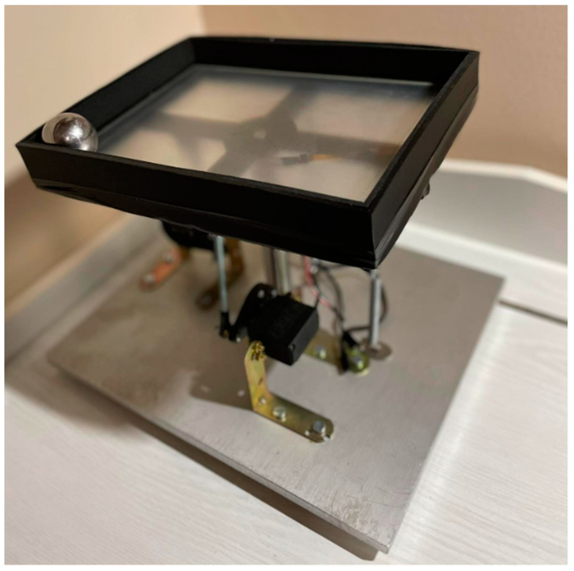
2.1. Physical Implementation

In terms of control, the movement in the two directions can be considered independent, so similar controllers can be applied on both axes. The main aspect during its implementation was that the position of the ball could be determined on the table, which forms an input for the neural network agent. The output of the agent is the degree of rotation of the table along the two axes.
The main characteristics of the physical system:
  • Maximum enclosure dimensions: H/W/W: 250/250/300 mm.
  • Touch panel: 225 × 173 mm.
  • Table angular adjustment accuracy: ±0.1 mm.
  • Table tilting speed as axis minimum: 0.3 s/60 °C.
  • At least 10 °C for angular rotation perpendicular to the X and Y axes.
Main features of the electrical system:
  • Application of low voltage system (<24 V).
  • Position can be determined in every 0.05 s.
  • Application of two servo motors for the angular rotation of the table.
Simplifications were made on the mathematical model of the physical system, such that the displacements of the ball in the X and Y directions on the table are considered independent of each other, so the movement in the X and Y directions can be modeled independently and identically. In the simplified one-dimensional model, the table is positioned using a servo motor, such that one end of an arm is attached to the servo motor and the other one to the table. In this model, the ball can only move along one line, therefore the degree of freedom of the system is one [30], as illustrated in Figure 2.
The notations of the mathematical model are shown in Table 1.
If the position of the servo motor changes, it results in an angular rotation of the table.
To model the system, the following simplifications were made [31]:
  • The connection between the ball and the table is continuous and non-slip.
  • The ball is completely homogeneous and regular.
  • Vibrations resulting from movement can be neglected.
The mathematical model of the system can be given using a simple equation of motion, which has a constant form frictionless incline.
a X = g × s i n α
a Y = g × s i n β
During the design of the system (see Figure 3), its dimensions and components have been chosen so that they do not affect portability. Additionally, it had to be able to withstand the forces caused by the large number of trials required by the neural network learning agent. The device is based on a 300 × 250 × 5 (Material designation: AlMgSi 1) aluminum plate, which provides sufficient stability and is easier to work with than, for example, stainless steel. The main shaft, which is made of turned stainless steel (Material quality: KO33) with an outer diameter of 20 mm and an internal thread at both ends, is connected to the base with an M10 screw at the bottom, and at the top with an M5 screw to the cardan joint. The DL3017 type servo motors manufactured by SRT are able to move the table with sufficient speed and precision. In terms of its operating range, it can produce an angular rotation between −90 and 90 °C, which far exceeds our requirements. Its adjustment speed is 0.15 s/60 °C, which also meets expectations.
As Figure 4 shows, the basis of the system is one Raspberry Pi 3B+, supported by one servo HAT and an Arduino nano board for analog signal processing.
The electrical connection is shown in Figure 4 and Table 2. The core of the system is a Raspberry Pi 3B+ minicomputer with a 1.4 GHz processor and 1 GB of DDR2 RAM, power supply 5VDC. Although it does not have a video card, it has HDMI output and 4 USB ports. Computing capacity of Raspberry Pi is 6,2 GFLOPS, the computing demand of the neural network (with layers of size 8, 256, 128, and 25 neurons, see Section 2.2 for more details) is:
i D Q N = ( n i n + n h 1 + n h 1   n h 2 + n h 2 + n h o u t ) 2
i D Q N = ( 8 + 256 + 256 + 128 + 128 + 25 ) 2 = 76032
i r a s p b e r r y = 6.2 10 9 76032 = 81544.61
where i D Q N is the Flops demand of neural network, and i r a s p b e r r y is the number of neural network executions possible within one second. Since the neural network agent is executed only once in every 0.05 s, the required number of operations is 20. The Raspberry Pi 3B+ has enough computational capacity.
Since Raspberry Pi’s clock signal generation does not allow for accurate and precise PWM signal generation, when setting the servo motor via the GPIO (General Purpose Input Output) outputs, “spikes” in the signal may occasionally be experienced, which greatly reduces the control accuracy. Therefore, a separate servo controller is required. For this purpose, the Raspberry HAT (Hardware Attached on Top) connector is used, to which an “Adafruit 16-Channel PWM/Servo” servo controller is connected. The servo controller can handle 16 servo motors and has a corresponding Python 3.8 software library, which can be used to control the servo motors.
To determine the position of the ball, a 10.4″ 4-wire resistive touch panel was installed, with an insulating/spacer layer between two pairs of conducting layers. The two pairs of conducting layers are charge carriers, the charge of which changes when pressed together, so it is possible to determine the position of the ball. Since the signal processing is performed in an analog way, the position tracking is fast enough for the task.
Figure 5 shows the connection of the four-wire touch panel. Each layer can be considered as a connection of two potentiometers, which can be read in such a way that by connecting a voltage to one leg of the panel, we can estimate the X and Y coordinates from the degree of voltage change on the corresponding leg [32].
The analog inputs of Arduino are 4 wires, each for one connection. It uses connections A1 and A3 as outputs, and connections A0 and A2 as inputs. Thus, when the position of the ball changes on the table, the resistance of the panel changes in proportion with it, this way modifying the output voltage. The panel acts as a voltage divider. To read the position, we fitted the coordinate system according to Figure 6 to obtain the coordinates in the Arduino program. The entire range is divided into 256 units in both the X and Y axes, and then the obtained value is shifted by 128, such that the center of the coordinate system is in the geometric center of the panel [33].
X = ( x r e a d 1024 / 256 ) 128
Y = ( y r e a d 1024 / 256 ) 128
The outer 5 mm of the panel is not taken into account when scanning, as the scanned values are uncertain there. The scanned values are then transmitted to the Raspberry via a serial communication port in text format. The Arduino sends the position data with a frequency of 200 Hz.
The inaccuracy of the scan is greatly influenced by the position of the ball on the table, the error rate on the outer edge of the panel is larger, according to the coordinate system it can be up to 30–50 mm. The degree of error at the center can be set between ±5 mm. This requires the application of a filter in the main program.
The RL agent is trained through a large number of trials. To prevent the ball from falling during the training, we applied a barrier on the sides of the plate, as shown in Figure 7. The ball diameter is R = 33.33 mm and the mass of the ball is m = 151 g.
The entire program has been written in Python, except the reading of the raw signal of the resistive panel that is written in the Arduino environment. The RL agent was implemented in the PyTorch deep-learning framework. The software also implements a virtual environment which can be used in-place of the real environment.
Filtering was applied on the ball position raw measurements to cope with noisy inputs and also to obtain speed estimates which served as additional input to the neural network agent. Two types of filters, Kálmán filter and a simple linear regression-based filter were tested, we obtained better results with the latter one. In case of linear regression, we considered position measurements of the last 0.2 s (~40 measurements with position measurement frequency of 200 Hz). After fitting, outlier measurements (with deviation greater than two times of the average deviation) were ignored, and a new line was fitted on the remaining points. The effect of this filtering approach is demonstrated in Figure 8.

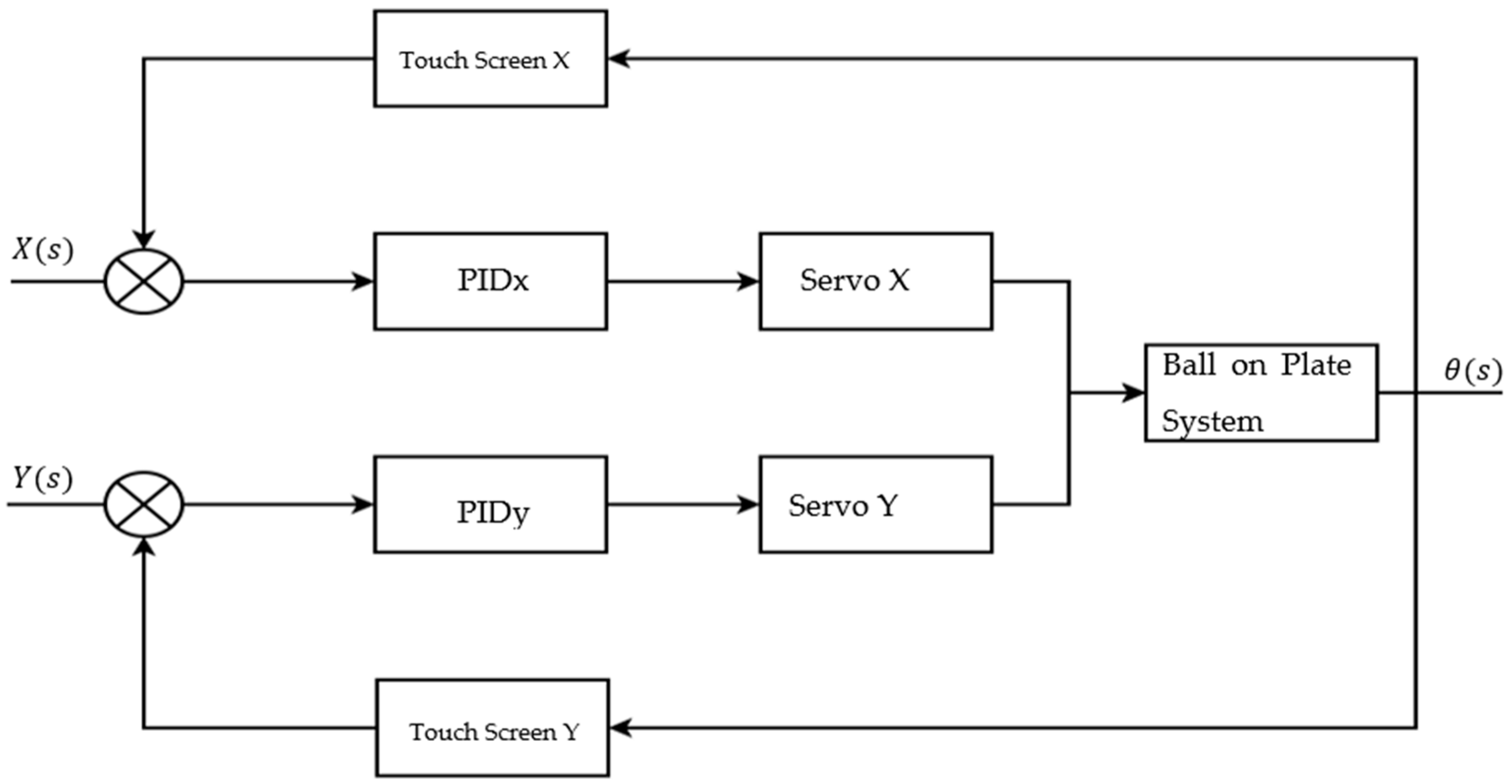
2.2. Control with Reinforcement Learning

Our goal was to examine the efficacy of reinforcement learning in controlling a real-world ball-on-plate balancing system. Reinforcement learning algorithms can be applied in environments in which an appropriate reward function can be defined. The rewards provide feedback to the agent on the goodness of its actions. In most cases, however, the reward is sparse and delayed, so effectiveness of a given action cannot be determined based only on the reward received right after performing an action. For example, in our case, it is difficult to determine how a slight modification of the inclination of the plate affects the future position of the ball. To cope with such sparse and delayed feedback, reinforcement learning algorithms seek to learn to maximize the expected cumulative future rewards.
To apply RL, first the action space had to be specified. The maximal angle of inclination of the plate was restricted to ±4 degrees in both directions. As the chosen learning algorithm is designed to output discrete actions, we divided the continuous ±4 degrees range into 40 units. At each time-step, the agent was allowed to modify the inclination by −2, −1, 0, +1, or +2 units, in both directions. Thus, the size of the action space was 5 × 5 = 25. Therefore, one output action of the agent can modify the inclination by 0, or 4 1 40 = 0.1 , or 4 2 40 = 0.2   degrees in both directions.
The software interface of the servo motors allows the motor position to be specified in degrees. The relation between motor positions and plate inclination is considered linear, the ±4 degrees plate inclination range in the two directions corresponded to motor position ranges ±9.17 degrees and ±17.19 degrees.
The update frequency of the system was 20 Hz, allowing the agent to update the state of the environment in every 0.05 s. We found that this setting allows the agent to perform both coarse interventions to drive the ball towards the center of the plate, and fine motions to keep the ball close to the center.
To make the balancing problem learnable for reinforcement learning algorithms, the reward function had to be defined. Although our only goal was to keep the ball close to the center of the plate, we found that defining the reward to simply be inversely proportional to the distance of the ball to the center is insufficient. The agent can achieve a relatively high cumulative reward by moving the ball back and forth between two opposite sides or opposite corners of the plate (note that for training, we applied rails on the edges of the plate to prevent the ball from falling). While this simple policy is suboptimal, it provides a high total reward and we found that the agent is not able to move towards the optimal solution.
Therefore, we complemented the reward function with a term that penalizes the speed of the ball (determined using the filter applied on the position measurements) and with another term that rewards the agent when the ball is located inside the central 25% of the area. More specifically, let denote (x, y) the 2-dimensional relative position of the ball, i.e., both x and y take values from [ 1 ,   1 ] . We also consider the 2D speed of the ball ( v x , v y ) , determined using filtering. The overall reward function can then be defined as:
R = K ( x 2 + y 2 ) ( v x 2 + v y 2 ) 0
where we set penalty K = 10 when | x | < 0.5 or | y | < 0.5 , and K = 0 , otherwise, while a 0 = max { a ,   0 } .
For the learning agent, the Deep Q-Network (DQN) [21] algorithm was chosen. It is implemented as a neural network which receives the state of the environment as input and outputs the so-called Q-values of the possible actions. The action corresponding to the maximal Q-value is chosen. Q-learning seeks a policy that maximizes the expected value of the total reward received in all the successive steps. The Q-value for a given state-action pair is defined by the following recursive function:
Q ( s , a ) = R ( s , a ) + γ m a x a Q ( s a ) ,
where s and a denote the current state and action, respectively, and s′ is the resulting state in the next time-step, while R ( s , a ) is the reward function.
In DQN, Q ( s , a ) is approximated by a neural network Q θ ( s , a ) with parameter vector θ . It is trained to minimize the following objective function (loss function):
E s , a , r , s [ Q θ ( s , a ) ( r + γ m a x a Q θ ( s , a ) ) ] 2
where the expectation is taken over state transitions (s, a, r, s′) collected from the environment through trials, see Figure 9.
We used a simple feedforward neural network with two hidden layers with 256 and 128 neurons, each neuron is followed by SiLU activation [34]. The eight neurons of the input layer received the two-dimensional position and speed of the ball, the current horizontal and vertical angle of inclination of the plate, and the previous action (horizontal and vertical modification of the inclination, in units). The network outputs the Q-values for the 25 possible actions.
To train the agent, we collected experiences by running trials of length 6 s (120 time-steps). After each trial, the neural network was updated by 64 training iterations using experiences collected in the last 50 trials. An Adam optimizer with a learning rate of 0.0001 and batch size of 64 was used. The discount factor “γ” in Equation (10) was set to 0.9, while we applied the “ε”-greedy strategy to explore the state–action space, “ε” decreased exponentially with power 0.9995 from 1.0 to 0.1. The pseudo-code of the learning method can be found in Algorithm 1. There was no predetermined maximum number of training steps, instead the training finished when the reward (averaged over the latest 100 episodes) stopped increasing. The received rewards and the value of the loss function in Equation (10) during training in the real environment can be seen in Figure 10. The increasing loss is not uncommon in RL as the Q-function in Equation (9) changes during training; because of that, the improving agent receives higher rewards. Therefore, it also increases the quadratic loss in Equation (10). Note, however, that when the reward peaks, the loss starts to decrease indicating that the agent is able to approximate the Q-function.
We followed this learning method in both virtual and real-world environments. To fine-tune a virtually pre-trained agent in the real-world environment, we decreased epsilon from 0.3 to 0.1.
Algorithm 1: Deep Q-Learning
1: Inputs: Episode length T, number of training iterations N, mini-batch size S, experience replay dataset size M, initial 𝜀, decay factor k, discount factor 𝛾
2: Output: Trained neural network Q θ
3: Initialize neural network Q θ and experience replay dataset D
4: Repeat
5:   # Trial phase
6:   Observe environment state s 1
7:    For t = 1..T  do
8:      With probability 𝜀 perform a random action a t
9:      otherwise perform a t   = a r g m a x a Q θ ( s t , a )
10:       Observe reward r and next environment state s t + 1
11:       Store transition ( s t , a t ,   r ,   s t + 1 ) in D
12:   Keep in D only transitions of the last M episodes
13:   # Training phase
14:   For N iterations do
15:      Sample a random transition mini-batch B = { ( s i , a i , r i ,   s i ) ,   i = 1 .. S } from D
16:      Compute loss according to Equation (10) using discount factor 𝛾
17:      Perform an optimization step using Adam optimizer
18:     𝜀 ← k𝜀
19: Until the averaged reward stops increasing
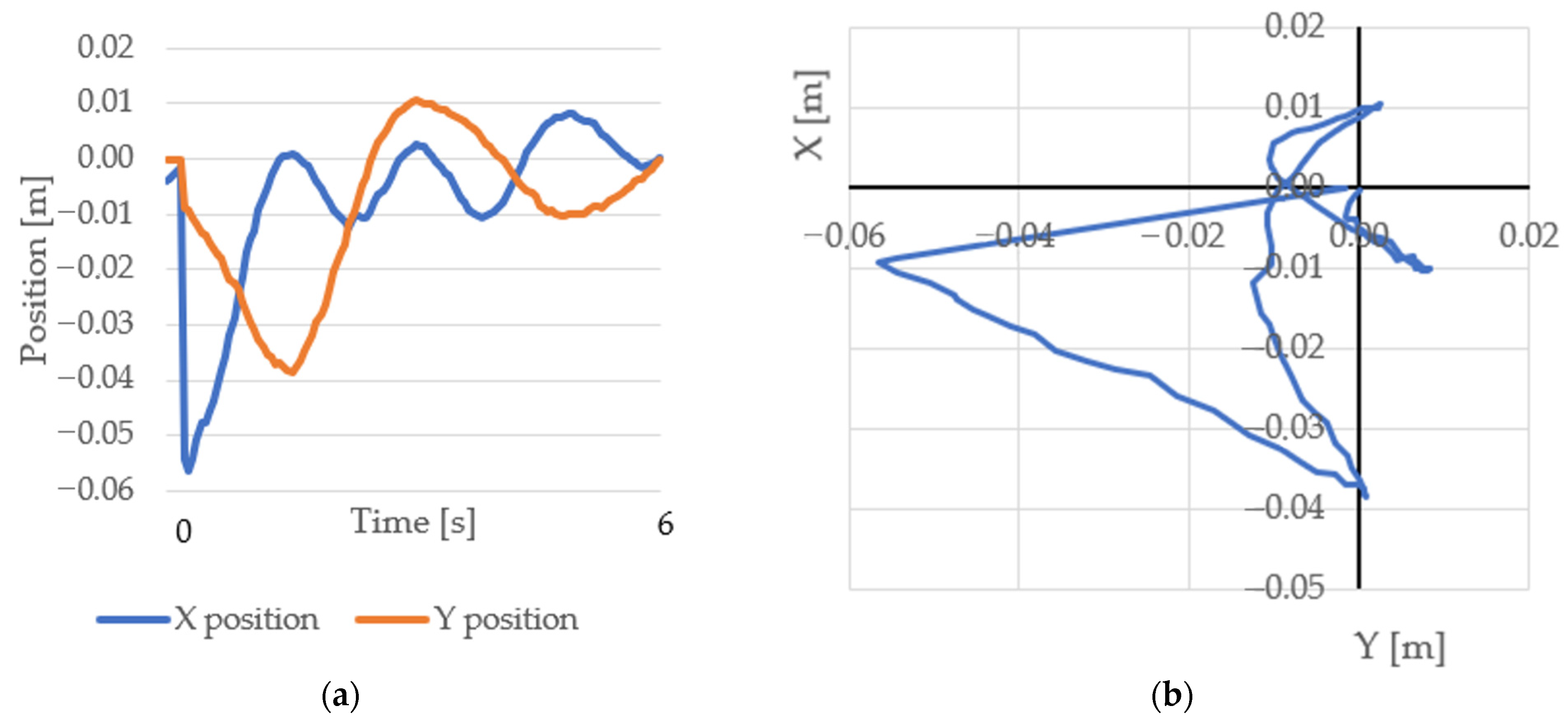
3. Results

DQN agents were trained in both the virtual and the real environments. As a third experiment, the former one was fine-tuned in the real environment. As the virtual environment mimics the dimensions and parameters of the real one, the results can be compared. Figure 10 shows that in the real environment around 3000 training iterations were required.
In the real environment, the learning takes about 6 h as one trial iteration takes 6 s. Contrary to this, in the virtual environment the training takes a few minutes and only around 1700 iterations are required. After virtual training, it required only 300 iterations in the real environment to fine-tune the agent. It means that the training time takes less than 1 h, in this case.
We tested both a virtually trained and a real-world-trained agent in the real environment. In both cases, the system managed to keep the ball on the table, but their accuracy and settling time is different. As Figure 11 shows, running the agent trained in the real environment, the system is able to keep the ball close to the center position.
For testing and evaluating the agents, we run 200 episodes of 6 s. In the case of the agent trained in the real environment, the average position error was X = 2.1 mm, Y = 2.0 mm. The average settling time was 3.4 s. The average ball speed on the table was v = 0.27 m/s.
When the agent was trained only in the virtual environment, as Figure 12 shows, in the real environment it was able to keep the ball on the plate; however, it drove and kept the ball far from the center, around the position Y = 4 cm, X = 6 cm. This inaccuracy was consistent through the test runs and can be attributed to the slight differences between the virtual and real environments, as well as to the uncertainty of the control and position measurement in the real environment.
After running 6 s long trials 200 times, the average position error was X = 45 mm, Y = 61 mm. The average settling time was 5.6 s, but never reached the center position. The average ball speed on the table is v = 0.3 m/s.
Figure 13 shows an example result, with the virtually trained agent after fine-tuning in the real environment. It shows that fine-tuning corrected the displacement error (Figure 12) of the virtually trained environment.
During 200 test episodes the average position error was X = 3.1 mm, Y = 5.7 mm. The average settling time was 2.8 s. The average ball speed on the table was v = 0.36 m/s.
Two separate PID controllers were applied individually to each axis, as Figure 14 shows. In this case, each axis works like a ball-and-beam system, PIDx is dedicated to the X axis, while PIDy is dedicated to the Y axis. After experimental fine tuning, the following parameters provided the best result: X and Y axes proportional gain Kpx = 0.75, Kpy = 0.8, X and Y axes integral gain Kix = 0.9, Kiy = 0.8 and X and Y derivative gain Kdx = 0.8, Kdy = 0.75. For more details on PID controllers refer to [16].
For comparison with the DQN methods, the general precision of the positionings and the ball speeds are similar with both methods, while the PID controller average settling time is two times faster. Figure 15 shows an example run using PID control on the system. We note that deviation of the centered plate from horizontal can also affect the accuracy of the PID controller. On the contrary, RL methods can easily adapt to such positioning inaccuracies.
During 100 test iterations with the PID controller the average position error was X = 2.1 mm, and Y = 2.2 mm. The average settling time was 1.3 s. The average ball speed on the table was v = 0.26 m/s.
Table 3 summarizes and compares the results achieved using the three neural network agents and the PID controller.

4. Discussion

The presented experiments show the difference between the three training methods. Training in the real environment is slow but provides more precise control. The positioning of a virtually trained agent is inaccurate in the real environment, probably due to differences between the two environments. Fine tuning the virtually trained agent can correct this inaccuracy and provide acceptable behavior, while requiring much less training time compared to when the agent is trained purely in the real environment.
The experiments show that applying a neural network to this task cannot compete in some respects, as better control time and settling accuracy can be achieved, for example, with a traditional PID. What can be said in favor of the use of the neural network is that it can potentially also be trained for tasks that traditional controllers cannot handle or would only be able to do with difficulty, such as balancing a body with an irregular geometry. It would also be worth trying to train the neural network to achieve other goals, e.g., to reach the highest possible speed with the ball (while avoiding falling) or to stop the ball placed on it on the table in the shortest possible time. We leave these directions for future research.
It turned out that it is very important to define the training objective of the neural network well, because an incorrectly chosen reward function can result in very slow learning and suboptimal policies that differ from the expected behavior.
In terms of control, it would be worthwhile to try mixed control methods that also use a neural network, as literature shows, the precision of the regulation and the setting time could be significantly reduced as a result.
Finally, we proved that a control implemented purely with RL works, it can be useful in places where the mathematical model is partially or fully unknown, but the learning process can be defined and supervised.

5. Conclusions

The result presented in this paper shows that controlling a non-linear real-world system only using reinforcement learning is possible.
The Raspberry Pi 3B+ card computer has enough computing capacity to run the neural network model that is capable of learning the task. To observe the ball position, the resistive touch panel is a good price/value sensor, although effective signal processing is important. Nevertheless, it was shown that an RL-based control can be realized in such a low-cost environment. From the mechanical implementation point of view, the real challenge was to build up the system without significant assembling inaccuracies.
Experiments showed that both real-world-trained and virtually trained RL agent can handle the task in the real environment, although the latter required fine-tuning in the real environment to correct displacements. Quantitative evaluation of the tests showed the differences between the methods. While training in a virtual environment is much faster, training in a real environment produced more accurate results.
In these experiments, the RL agent was found to be inferior to a PID controller in terms of settling time. However, RL could possibly also be trained for tasks that traditional controllers cannot handle or would only be able to do with difficulty. This can be a topic for future research.

Author Contributions

Conceptualization, D.K., J.N. and J.S.; writing—review and editing, D.K., J.N. and J.S. All authors have read and agreed to the published version of the manuscript.

Funding

This research received no external funding.

Institutional Review Board Statement

Not applicable.

Informed Consent Statement

Not applicable.

Data Availability Statement

Data sharing not applicable. No new data were created or analyzed in this study. Data sharing is not applicable to this article.

Conflicts of Interest

The authors declare no conflict of interest.

References

  1. Shorya, A.; Bernard, N.; Boklud, A.; Master, D.; Ueda, K. Mechatronic design of a ball-on-plate balancing system. Mechatronics 2022, 12, 217–218. [Google Scholar]
  2. Zeeshan, A.; Nauman, A.; Jawad Khan, M. Design, Control and Implementation of a BaIlon Plate Balancing System. In Proceedings of the 2012 9th International Bhurban Conference on Applied Sciences & Technology (IBCAST), Islamabad, Pakistan, 9–12 January 2012; pp. 22–26. [Google Scholar] [CrossRef]
  3. Debono, A.; Bugeja, M. Application of Sliding Mode Control to the Ball and Plate Problem. In Proceedings of the 2015 12th International Conference on Informatics in Control, Automation and Robotics (ICINCO), Colmar, France, 21–23 July 2015; pp. 412–419. [Google Scholar]
  4. Bdoor, S.R.; Ismail, O.; Roman, M.R.; Hendawi, Y. Design and implementation of a vision-based control for a ball and plate system. In Proceedings of the 2016 2nd International Conference on Industrial Engineering, Applications and Manufacturing (ICIEAM), Chelyabinsk, Russia, 19–20 May 2016; pp. 1–4. [Google Scholar] [CrossRef]
  5. Castro, R.D.; Flores, V.J.; Salton, A.T.; Pereira, L.F.A. A Comparative Analysis of Repetitive and Resonant Controllers to a Servo-Vision Ball and Plate System. IFAC Proc. Vol. 2014, 47, 1120–1125. [Google Scholar] [CrossRef] [Green Version]
  6. Wettstein, N. Balancing a Ball on a Plate Using Stereo Vision. Master’s Thesis, Institute for Dynamic Systems and Control Swiss Federal Institute of Technology (ETH), Zurich, Switzerland, 2013; pp. 2–10. [Google Scholar]
  7. Bang, H.; Lee, Y.S. Implementation of a Ball and Plate Control System Using Sliding Mode Control. IEEE Access 2018, 6, 32401–32408. [Google Scholar] [CrossRef]
  8. Borelli, F. Ball and Plate. Constrained Optim. Control Linear Hybrid Syst. 2003, 290, 177–183. [Google Scholar]
  9. Kopichev, M.M.; Puov, V.A.; Pashenko, N.A. Ball on the plate balancing control system. In IOP Conference Series: Materials Science and Engineering, Proceedings of the 2nd International Conference on Aeronautical, Aerospace and Mechanical Engineering Prague, Czech Republic, 26–28 July 2019; IOP Publishing: Bristol, UK, 2019; Volume 638, p. 012004. [Google Scholar] [CrossRef]
  10. Zhou, A.; Leuken, R.; Arriens, H.J. Modeling A Configurable Resistive Touch Screen System Using SystemC and SystemC-AMS. In Proceedings of the 20th Annual Workshop on Circuits, Systems and Signal Processing-ProRISC, Veldhoven, The Netherlands, 26–27 November 2009; pp. 393–398. [Google Scholar]
  11. Lin, C.-L.; Chang, Y.-M.; Hung, C.-C.; Tu, C.-D.; Chuang, C.-Y. Position Estimation and Smooth Tracking With a Fuzzy-Logic-Based Adaptive Strong Tracking Kalman Filter for Capacitive Touch Panels. IEEE Trans. Ind. Electron. 2015, 62, 5097–5108. [Google Scholar] [CrossRef]
  12. Xiyang, L.; Feng, S.; Xianmei, C.; Jinrong, L.; Yaochi, Z. Research Technologies of Projected Capacitive Touch Screen. In Proceedings of the 5th International Conference on Computer Sciences and Automation Engineering, Sanya, Hainan, China, 14–15 November 2015; pp. 63–69. [Google Scholar]
  13. Galvan-Colmenares, S.; Moreno-Armendáriz, M.A.; Rubio, J.J.; Ortíz-Rodriguez, F.; Yu, W.; Aguilar-Ibáñez, C.F. Dual PD Control Regulation with Nonlinear Compensation for a Ball and Plate System. Math. Probl. Eng. 2014, 2014, 894209. [Google Scholar] [CrossRef] [Green Version]
  14. Mochizuki, S.; Ichihara, H. I-PD controller design based on generalized KYP lemma for ball and plate system. In Proceedings of the 2013 European Control Conference (ECC), Zurich, Switzerland, 17–19 July 2013; pp. 2855–2860. [Google Scholar] [CrossRef]
  15. Colmenares, S.G.; Moreno-Armendáriz, M.A.; Yu, W.; Rodriguez, F.O. Modeling and nonlinear PD regulation for ball and plate system. In Proceedings of the World Automation Congress, Puerto Vallarta, Mexico, 24–28 June 2012; pp. 1–6. [Google Scholar]
  16. Jadlovská, A.; Jajčišin, Š. Modelling and pid control design of nonlinear educational model ball & plate. In Proceedings of the 17th International Conference on Process Control 2009, Štrbské Pleso, Slovakia, 9–12 June 2009; pp. 475–483. [Google Scholar]
  17. Lo, J.H.; Wang, P.K.; Huang, H.P. Reinforcement Learning and Fuzzy PID Control for Ball-on-plate Systems. In Proceedings of the International Automatic Control Conference (CACS), Kaohsiung, Taiwan, 3–6 November 2022; pp. 1–6. [Google Scholar] [CrossRef]
  18. Hadoune, O.; Benouaret, M. Fuzzy-PID tracking control of a ball and plate system using a 6 Degrees-of-Freedom parallel robot. In Proceedings of the 19th International Multi-Conference on Systems, Signals & Devices (SSD), Sétif, Algeria, 6–10 May 2022; pp. 1906–1912. [Google Scholar] [CrossRef]
  19. Li, J.-F.; Xiang, F.H. RBF Network Adaptive Sliding Mode Control of Ball and Plate System Based on Reaching Law. Arab. J. Sci. Eng. 2021, 47, 9393–9404. [Google Scholar] [CrossRef]
  20. Kan, D.; Xing, B.; Xie, W. A minimum phase output based tracking control of ball and plate systems. Int. J. Dyn. Control. 2022, 10, 462–472. [Google Scholar] [CrossRef]
  21. Zheng, Q.; Yang, M.; Yang, J.; Zhang, Q.; Zhang, X. Improvement of Generalization Ability of Deep CNN via Implicit Regularization in Two-Stage Training Process. IEEE Access 2018, 6, 15844–15869. [Google Scholar] [CrossRef]
  22. Jin, B.; Cruz, L.; Gonçalves, N. Pseudo RGB-D Face Recognition. IEEE Sens. J. 2022, 22, 21780–21794. [Google Scholar] [CrossRef]
  23. Yao, T.; Qu, C.; Liu, Q.; Deng, R.; Tian, Y.; Xu, J.; Jha, A.; Bao, S.; Zhao, M.; Fogo, A.B.; et al. Compound Figure Separation of Biomedical Images with Side Loss. In Deep Generative Models, and Data Augmentation, Labelling, and Imperfections, Proceedings of the First Workshop, DGM4MICCAI 2021, and First Workshop, DALI 2021, Held in Conjunction with MICCAI 2021, Strasbourg, France, 1 October 2021; Springer: Berlin/Heidelberg, Germany, 2021; Volume 13003, pp. 173–183. [Google Scholar]
  24. Zhao, M.; Liu, Q.; Jha, A.; Deng, R.; Yao, T.; Mahadevan-Jansen, A.; Tyska, M.J.; Millis, B.A.; Huo, Y. VoxelEmbed: 3D Instance Segmentation and Tracking with Voxel Embedding based Deep Learning. In Machine Learning in Medical Imaging, Proceedings of the 12th International Workshop, MLMI 2021, Held in Conjunction with MICCAI 2021, Strasbourg, France, 27 September 2021; Springer: Berlin/Heidelberg, Germany, 2021; Volume 12966, pp. 437–446. [Google Scholar]
  25. Mnih, V.; Kavukcuoglu, K.; Silver, D.; Rusu, A.A.; Veness, J.; Bellemare, M.G.; Graves, A.; Riedmiller, M.; Fidjeland, A.K.; Ostrovski, G.; et al. Human-level control through deep reinforcement learning. Nature 2015, 518, 529–533. [Google Scholar] [CrossRef]
  26. Dulac-Arnold, G.; Levine, N.; Mankowitz, D.J.; Li, J.; Paduraru, C.; Gowal, S.; Hester, T. Challenges of real-world reinforcement learning: Definitions, benchmarks and analysis. Mach. Learn. 2021, 110, 2419–2468. [Google Scholar] [CrossRef]
  27. Pan, X.; You, Y.; Wang, Z.; Lu, C. Virtual to Real Reinforcement Learning for Autonomous Driving. In Proceedings of the BMVC 2017, London, UK, 4–7 September 2017. [Google Scholar]
  28. Hasselt, H. Double Q-learning. Adv. Neural Inf. Process. Syst. 2011, 23, 2613–2622. [Google Scholar]
  29. Dewey, D. Reinforcement Learning and the Reward Engineering Principle. In Proceedings of the AAAI Spring Symposia, Palo Alto, CA, USA, 24–26 March 2014. [Google Scholar]
  30. Ball & Beam: Simulink Modeling. Available online: https://ctms.engin.umich.edu/CTMS/index.php?example=BallBeam&section=SimulinkModeling (accessed on 18 November 2022).
  31. Nokhbeh, M.; Khashabi, D. Modelling and Control of Ball-Plate System. Final Project Report; Amirkabir University of Technology: Tehran, Iran, 2011; pp. 1–15. [Google Scholar]
  32. 4-Wire and 8-Wire Resistive Touch-Screen Controller Using the MSP430. Available online: http://dangerousprototypes.com/blog/2012/01/07/4-wire-and-8-wire-resistive-touch-screen-controller-using-the-msp430/ (accessed on 18 November 2022).
  33. Kóczi, D. Neurális Hálóval Vezérelt Kétdimenziós Pozícionáló Megtervezése és Kivitelezése. Master’s Thesis, University of Szeged, Szeged, Hungary, 2019. [Google Scholar]
  34. Elfwing, S.; Uchibe, E.; Doya, K. Sigmoid-weighted linear units for neural network function approximation in reinforcement learning. Neural Netw. 2018, 107, 3–11. [Google Scholar] [CrossRef] [PubMed]
Figure 1. Ball-On-Plate illustration.
Electronics 12 00671 g001
Figure 2. Kinematic diagram of a one-dimensional model.
Electronics 12 00671 g002
Figure 3. Ball-on-plate system dimensions [mm].
Electronics 12 00671 g003
Figure 4. Ball-on-plate system dimensions.
Electronics 12 00671 g004
Figure 5. Resistive touch-screen wiring diagram.
Electronics 12 00671 g005
Figure 6. Resistive touch-screen coordinate system.
Electronics 12 00671 g006
Figure 7. Physical implementation.
Electronics 12 00671 g007
Figure 8. Example filtering result.
Electronics 12 00671 g008
Figure 9. State-transition experiences are collected during trials (left). These experiences are then used to train the agent (right).
Electronics 12 00671 g009
Figure 10. Training in a real environment. Average rewards collected in each trial are shown. Through experience, we found that an average reward of ~7 meant that the agent was able to keep the ball close to the center.
Electronics 12 00671 g010
Figure 11. (a) Example run: X and Y positions in the real environment using an agent trained in the real environment; (b) position accuracy in 2 dimensions.
Electronics 12 00671 g011
Figure 12. (a) Example run: X and Y positions in the real environment using a virtually trained agent. (b) Positions in 2 dimensions.
Electronics 12 00671 g012
Figure 13. (a) Example run: X and Y positions in the real environment using a pre-trained and fine-tuned agent; (b) positions in 2 dimensions.
Electronics 12 00671 g013
Figure 14. PID control system design.
Electronics 12 00671 g014
Figure 15. (a) Example run: X and Y positions in the real environment using PID control; (b) Positions in 2 dimensions.
Electronics 12 00671 g015
Table 1. Notations.
Table 1. Notations.
NotationDescription
mball mass
Rball diameter
dshaft length
ggravitational acceleration
Ltable length
hball position
aXBall acceleration X component
aYBall acceleration Y component
α–alphatable tilt angle-X
β–betatable tilt angle-Y
Θ–thetatilt angle of servo motor
Table 2. Electrical components.
NumberDescription
1Raspberry Pi 3B+
2Adafruit 16C PWM HAT
3Arduino UNO Rev3
4DL3017 LV Digital Servo
510.4″ Resistive touch panel (4 wire)
6Power supply: 5 V DC 3.0 A
7Power supply: 5 V DC 2.1 A
Table 3. Comparison of different training methods and PID.
NameReal TrainedVirtually TrainedVirtually Trained after Fine-TuningPID
Average Position error X [mm]2.1453.12.1
Average Position error Y [mm]2615.72.2
Average Settling time [s]3.45.62.81.3
Average Ball speed [m/s]0.270.30.360.26
Disclaimer/Publisher’s Note: The statements, opinions and data contained in all publications are solely those of the individual author(s) and contributor(s) and not of MDPI and/or the editor(s). MDPI and/or the editor(s) disclaim responsibility for any injury to people or property resulting from any ideas, methods, instructions or products referred to in the content.

