XDLL: Explained Deep Learning LiDAR-Based Localization and Mapping Method for Self-Driving Vehicles

Abstract

Self-driving vehicles need a robust positioning system to continue the revolution in intelligent transportation. Global navigation satellite systems (GNSS) are most commonly used to accomplish this task because of their ability to accurately locate the vehicle in the environment. However, recent publications have revealed serious cases where GNSS fails miserably to determine the position of the vehicle, for example, under a bridge, in a tunnel, or in dense forests. In this work, we propose a framework architecture of explaining deep learning LiDAR-based (XDLL) models that predicts the position of the vehicles by using only a few LiDAR points in the environment, which ensures the required fastness and accuracy of interactions between vehicle components. The proposed framework extracts non-semantic features from LiDAR scans using a clustering algorithm. The identified clusters serve as input to our deep learning model, which relies on LSTM and GRU layers to store the trajectory points and convolutional layers to smooth the data. The model has been extensively tested with short- and long-term trajectories from two benchmark datasets, Kitti and NCLT, containing different environmental scenarios. Moreover, we investigated the obtained results by explaining the contribution of each cluster feature by using several explainable methods, including Saliency, SmoothGrad, and VarGrad. The analysis showed that taking the mean of all the clusters as an input for the model is enough to obtain better accuracy compared to the first model, and it reduces the time consumption as well. The improved model is able to obtain a mean absolute positioning error of below one meter for all sequences in the short- and long-term trajectories.

1. Introduction

A self-driving vehicle requires more attention to be paid to the execution time of their components, since this may save many lives every day [1]. It must be ready to perform the right action in real time to prevent incidents. In order to achieve this level of control, the system should be built to provide rapid interaction between its components, to receive instant location information to perform the overtaking of vehicles and perform rapid path planning [2]. Localization of the vehicles is an essential step to ensure the functionality of other components. The information provided can be used to identify the distances between the vehicles and the structures in the environment, which is crucial information needed to avoid collisions, find the shortest distance to the destination, and so on [2]. Global navigation satellite systems (GNSS) are already equipped, in almost all autonomous vehicles, to provide position coordinates by triangulation using at least three satellites. However, this technology faces several issues for real-time execution when the satellite signals are interrupted, such as under bridges, in tunnels, and around tall buildings [3,4]. Several researchers have thought to localize the vehicle based on internal sensors, such as light detection and ranging (LiDAR), cameras, inertial measurement units (IMUs), or even radar sensors [2].

Our review of the state-of-art in this area divides the related methods into two categories: direct methods and feature-based methods. Direct methods try to estimate vehicle’s position directly by calculating the distances between two positions and using dead reckoning (DR) to deduce the position. The IMU unit from the inertial navigation system (INS) is one of the methods that uses this approach [5]. An IMU provides information about the acceleration and attitude rate of the vehicle. The double integration of the acceleration measurement will provide the position of the vehicle. However, the double integration is prone to errors that can be accumulated during the execution of the process [5]. Several researchers have tried to correct these errors by sending them to a machine learning model, such as an input delay neural network (IDNN) [6], multi-layer feed forward neural network (MFNN) [7], recurrent neural network (RNN) [8], or long short-term memory (LSTM) model [9,10]. For more information about deep learning (DL) methods in self-driving vehicles, the readers are referred to [11].

Wheel odometry is a great tool for estimating the vehicle’s position that works by using the velocity and integrating it to get the position [12]. However, as we mentioned before, the integration process provides an error that can be amplified and accumulated each time we re-execute the process. According to the article [12], using wheel odometry is better than using an IMU accelerometer, since it needs less integration time. The wheel odometry neural network (WhONet) [12] uses an RNN-based architecture to correct the wheel odometry errors, and an extensive experiment was performed during several GNSS outages.

Feature-based approaches for vehicle localization try to extract relevant features from data gathered from one or more sensors. We have surveyed in this work only LiDAR-based methods, since we believe that the camera images are easily affected by weather changes such as snow and rain [1,2]. Extracting features from LiDAR measurements has been the subject of several papers in the literature. LiDAR odometry and mapping (LOAM) [13] distinguish edges and flat plan features to perform scan-to-scan and scan-to-map matching, which are techniques to track the vehicle’s motions (translation and rotation) between consecutive sequences. However, the process consumes too much time when executed, which is covered in the article introducing the LOAM_Velodyne [14] method. To solve the same issue, lightweight and ground-optimized LOAM (LeGO-LOAM) [15] and A-LOAM [16] approaches remove noisy and useless features to reduce the computational time. Other methods, such LO-Net [17] and LO-Net-M [17], use end-to-end deep learning (DL) to improve the scan-to-matching process. SGLO [18] extracts geometric line and plane features to improve the matching process, which has provided good results. However, the accuracy is dramatically affected by the initialization. Methods such as those of Kummerle et al. [19], Weng et al. [20], Sefati et al. [21], and A. Schaefer et al. [22] use a probabilistic perspective to localize the vehicles. Based on detecting poles and walls from LiDAR scans, the methods used a particle filter algorithm to correct the IMU’s accumulative errors. The method of Schaefer et al. [22] achieved excellent results on the Kitti dataset [23] and the University of Michigan North Campus Long-Term Vision and LiDAR Dataset (NCLT) [24]. However, the features extracted for the operation may not exist in some environments, especially those with little in the way of texture, such as desert roads. That is why the work of Charroud et al. [25] proposed using non-semantic features to help perform the measurement-update step in the particle filter. An extension of this work was presented in the article [26], where the authors proposed a modified clustering particle filter that selects relevant particles to calculate the position by using sigma-point selection. Moreover, another extension of the work in [25] is the article [27], where it was proposed to extend the work on particle filters by selecting only the 10 best particles around the real position and regenerating the particles around them. This trick enables the particle filter to run fast and preserves the accuracy, as we generate particles close to the real position at each execution of the algorithm.

Our novel method uses non-semantic features as a pre-processing step to teach a machine-learning model the actual vehicle positions. The inputs are the extracted features, and the outputs are the positions. The model was extensively tested on short- and long-term trajectories using two benchmark datasets: Kitti [23] and NCLT [24]. In addition, the model is explained by studying the features that contribute positively or negatively to the output model. Based on the results of explaining the first model, another model was constructed and compared to evaluate the influence of the changes made. The article [28] discusses the concept of explainable artificial intelligence (XAI), which refers to the development of AI systems that are able to provide clear, interpretable explanations for their decisions and actions. The authors provide an overview of the various types of XAI approaches that have been proposed, including post hoc explanation methods, integrated explanation methods, and interactive explanation methods. They also explore the potential benefits and challenges of XAI, and discuss the importance of responsible AI development in ensuring the transparency, accountability, and trustworthiness of AI systems.

This paper contains the following contributions:

• As far as the authors are aware, this is the first method that uses only a few LiDAR cluster points to feed a deep-learning model for localization purposes.
• The paper presents, in Section 2, a robust mathematical formulation of the localization problem, which opens up some opportunities to develop more solutions based on optimization and stochastic-differential-equation-based methods.
• Deep Learning explanation methods were employed to find the most contributing cluster features in order to optimize the proposed model.

The sections of the paper are organized as follows. Section 2 provides an in-depth explanation of the problem and the architecture we propose to solve it. Section 3 presents the steps followed to create the proposed model. Section 4 presents the results of testing the model in the short and long-term scenarios. The contributions of the features are also discussed, and a comparison between the two models with further implications is presented in this section. Section 5 provides some conclusions.

2. Problem Description and Proposed Architecture

As mentioned before, any autonomous system requires a localization and mapping method to facilitate the scheduling of other principal tasks, such as path planning and overtaking vehicles. [1]. In particular, self-driving vehicles must be given more attention regarding the execution times of different components, since they need an instant interaction with the environment, which means that we need to ensure fast execution of the methods without hurting the accuracy too much. Quickness and accuracy are critical to getting a better experience from driving. Most of the state-of-the-art methods divide the process of localization and mapping into two parts: feature extraction and localization prediction. Extracting relevant features is a principal task in creating a global map, and helps to execute the localization task easily by providing the environmental objects or shapes around the vehicles. Figure 1 presents a simple workflow architecture that consists of two major steps: feature extraction (A) and learning the positions (B). In this section, we want to give the theoretical intuitions about the approaches followed to solve the localization and mapping problem for self-driving vehicles, which could be extended to other autonomous systems. A practical implementation of the method is delivered in the next section.

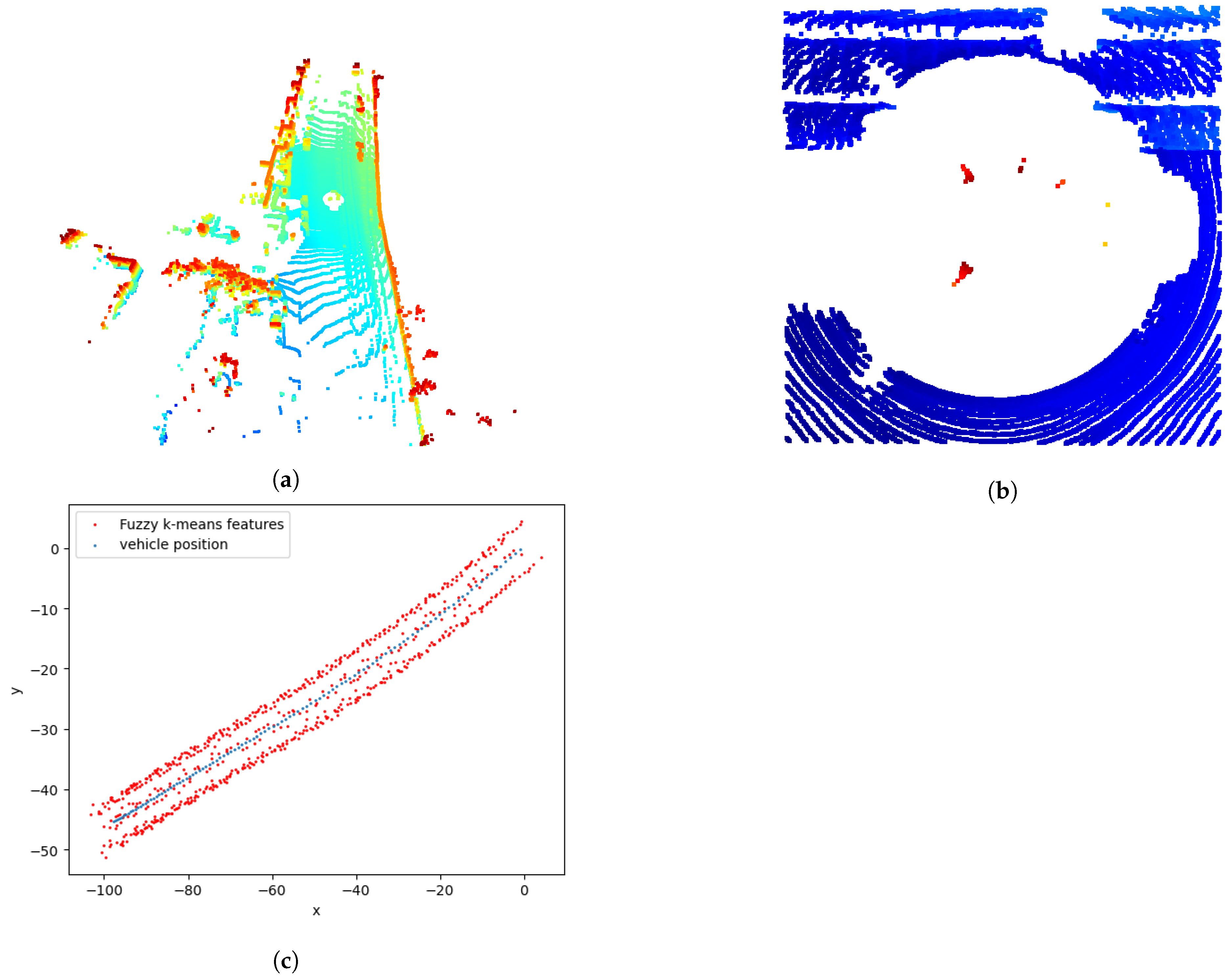
Our method localizes the vehicle based on LiDAR measurements only. We suppose that the LiDAR scans and the ground truth positions are in the body-frame coordinates, where at each timestamp each position has its corresponding scan. We use non-semantic features to distinguish some relevant prototype features. This technique can represent a wide range of objects inside the environment, in contrast to focusing on a single object (such as poles or edges), which is very advantageous to representing environments with less texture information. We chose to employ a clustering algorithm to extract clusters, which form our non-semantic features.

Let us have some mathematical formulation:

Let $P_t$ be a LiDAR scan at time t:

$$P_t={\left\{p_{t,i}\right\}}_{i\in [1,D_t]}\mathrm{where}{p}_{t,i}=[x_i,y_i,z_i]$$

(1)

where $D_t$ is the number of LiDAR points at time t, and let also $s_t=[s_{t,i},s_{t,j}]$ be the real position at time t (the z coordinate is supposed to be the same for the real position). We apply a clustering technique by fixing the number of centers to a certain value (discussed in the next section), so we have:

$$C_t={\left\{c_{t,i}\right\}}_{i\in [1,D_t^{\prime }]}\mathrm{where}{c}_{t,i}=[x_{t,i}^{\prime },y_{t,i}^{\prime },z_{t,i}^{\prime }]$$

(2)

and $D_t^{\prime }$ is the number of clusters, $C_t$ is the group of center clusters, and $c_{t,i}$ is the center of cluster i, where $i\in [i,D_t^{\prime }]$. For simplicity, below we consider that the number of clusters stays the same along the trajectory ($D^{\prime }=D_t^{\prime }$ for all t).

The main idea of this paper is to find $\{{\alpha }_{t,1},{\alpha }_{t,2},...,{\alpha }_{t,D^{\prime }}\}$ and a function f that will minimize the problem $\left(p\right)$:

$$\left(p\right):\left\{\begin{array}{c}Min(\sum _{t=1}^T\sum _{i=1}^{D^{\prime }}\parallel {\alpha }_{t,i}f(w_{t,i},c_{t,i})-s_t){\parallel }_2^2)\\ w_{t,1},\dots ,w_{t,D^{\prime }}\in R^{+}\\ {\alpha }_{t,1},\dots ,{\alpha }_{t,D^{\prime }}\in R^{+}\end{array}\right.$$

(3)

T is the last timestamp value. We try to estimate a function f that will aggregate and manipulate the centers’ clusters $C_t={\left\{c_{t,i}\right\}}_{i\in [1,D^{\prime }]}$ in order to get an estimated position that will be close to the real position $s_t$. $w_{t,i}$ are some weights to ensure the reliability of the projection of the cluster from the 3D to the 2D environment. Scalars $\left\{{\alpha }_{t,i}\right\}$ are used to provide a percentage (probability) of the importance of the clusters $\left\{c_{t,i}\right\}$ after manipulation with the function f.

To solve the problem $\left(p\right)$, we established a method based on a deep learning approach that takes the cluster features as the input and returns back the estimated positions. The architecture was chosen manually by testing the capabilities and robustness of several time series regression methods, such as LSTM, GRU, and RNN. We envisaged that the proposed architecture in Figure 2 is robust enough to learn and predict unseen data—i.e., that it has the capacity for generalization. The reader may remark that several convolutions were applied to eliminate the data outliers. LSTM and GRU are the main layers to create the memory inside the proposed model. We have demonstrated the capacity of this architecture by testing on several popular time-series methods.

Table 1. Comparing several models to choose the best architecture.

Time Series Method	Training MAE	Validation MAE
LSTM	0.93	0.92
GRU	0.79	0.77
RNN	0.84	0.86
LSTM and RNN	0.86	0.86
GRU and RNN	0.76	0.77
OURs	0.75	0.75

presents the results of comparing the training and validation MAE (mean absolute error) of our method and other architectures.

3. Datasets and Parameters

3.1. Selection of Datasets

In order to train and test the model, we have used sequences from two popular benchmarks: Kitti [23] and Michigan North Campus Long-Term (NCLT) [24] datasets.

• Kitti Dataset: This dataset provides the opportunity to train the model in different categories provided in the dataset, including city, residential, road, campus, and person. This appropriate dataset enables also teaching the model in various challenging environments and investigating the performance of vehicles in short-term localization trajectories.
• NCLT Dataset: The North Campus Long-Term (NCLT) dataset was acquired with a Segway robot on one of the campuses of the University of Michigan, USA. It is a great option for training and testing the model’s performance, since it contains long-term trajectory sequences with an average length of 5.5 km over a period of 15 months. The recordings included different times of day; different weather conditions; seasonal changes; indoor and outdoor environments; many dynamic objects, such as people and moving furniture; and two large, constantly changing construction projects. Although the trajectories vary considerably from session to session, there is considerable overlap.

Both datasets provide the information needed to train and test the model; the LiDAR point cloud was converted to the reference system, and ground truth of the positions was created based on GPS or/and a SLAM solution using LiDAR scan matching and high-accuracy RTK GPS. We have carefully distinguished sequences that have different sizes and contain various environmental scenarios, such as hard brakes, roundabouts, town drives, residential road drives, dirt roads, traffic, and sharp cornering, in order to teach robustly, as much as possible, the driving scenarios to the model.

Table 2. The sequences used to train the model.

Sequence	Dataset	Date	Frames Num	Kilometer
00	Kitti	2011-10-03	4544	- 1
05	Kitti	2011-09-30	2762	- 1
06	Kitti	2011-09-30	1104	- 1
07	Kitti	2011-09-30	1106	- 1
08	Kitti	2011-09-30	5177	- 1
09	Kitti	2011-09-30	1594	- 1
10	Kitti	2011-09-30	1224	- 1
00	NCLT	2012-01-08	28,127	6.4
25	NCLT	2013-01-10	5120	1.1
SUM	–	–	50,758	–

¹ The Kitti dataset did not mention the kilometers of driving the vehicles either in its official website or in its paper.

depict the sequences used to train the model, which contain in total 50,758 units of LiDAR scans (data input) and ground truth (target) with different velocity variations.

3.2. Data Processing and Parameters’ Discussion

In this part, we have manipulated the data (input and target) to teach the model the vehicle’s real positions (target) based on the features extracted from the LiDAR scan at each timestamp (input):

• Processing the target: Each dataset used here provides the ground truth of the vehicle positions. Along the trajectory, each timestamp of the position should coincide with the LiDAR scan timestamp or at least should be close to it (see Figure 3).
• Processing the input data: In order to prepare meaningful inputs for the model, a feature-extraction process had to be employed for each LiDAR scan to reduce the huge amount of points it contains. First, we performed a “cropping” step that cut the scan to keep only the region of interest. We kept only the points that surround the vehicle and do not exceed the height of the vehicle. In fact, we manually distinguished the points that respect these constraints, as seen in Figure 4b:
  Let $P_t=[x_t,y_t,z_t]$ be a LiDAR point from the scan t:

  $$\begin{array}{c}\hfill -10\mathrm{m}\le x_t\le 10\mathrm{m}\\ \hfill -10\mathrm{m}\le y_t\le 10\mathrm{m}\\ \hfill z_t\le 0.5\mathrm{m}\end{array}$$
  These limits were carefully chosen to ensure some overlap between scans. In addition, a fuzzy k-means clustering algorithm was performed to extract features from each cropped scan. The use of a clustering technique summarizes the LiDAR information into some core groups that are useful for explaining objects in the environment, e.g., trees, poles, and walls.

  Table 3. Time consumption (mm: ss) to execute the feature extraction for different clustering methods tested on the sequence 0001 from the Kitti dataset [23].

  Clustering Method	Time Cost
  KMeans	00:08
  Fuzzy k-means	00:07
  Gaussian mixture model	00:08
  DBSCAN	00:10
  Particle Swarm Optimized Clustering	00:09

  highlights how fast fuzzy k-means clustering is and that it is a good choice for this task, which is also proven in the article [25].
  We decided to run the feature-extraction process with five center clusters, since the number of frames is big and each LiDAR frame (scan) contains a massive number of points, e.g., millions of points. Consequently, the calculation time will be huge if we choose a bigger number of clusters. However, we will analyze the contribution of each cluster (or feature) to the output model in the next section.
  After calculating the five center cluster features at each scan, we calculate the mean of all those clusters and add it to the input as the sixth feature. Figure 5 provides an illustration of the inputs of our model, and Figure 4 illustrates an example of the following data processing step.

3.3. Training the Model

• Parameter tuning:
  Finding the best parameter configuration is a crucial step to ensure the best accuracy with the minimum time cost, which is well needed for machine-learning applications. Self-driving vehicles require a fast and accurate positioning method to work in real-time. We have used a random algorithm that optimizes the parameters by selecting random parameters after defining a range for each of them [29].

  Table 4. Parameter tuning for the model.

  Layer	Range of Choice	Best Choice
  ConvLSTM1D	[32, 130] 1	32
  LSTM	[32, 130] 1	96
  conv1D	[32, 130] 1	96
  GRU	[32, 130] 1	128
  activationLSTM	[“elu”, “linear”, “tanh”]	tanh
  activationGRU	[“elu”, “linear”, “tanh”]	elu
  IsDropout	[True, False]	False
  learning rate	[${10}^{-4}$, ${10}^{-2}$]	0.0003

  ¹ 32 is the step size used here.

  depicts the results found after running 100 random trials. The best parameter combination achieved 1.21 m of the MAE in less than 30 s of training running. The choice of the optimization method was done manually by testing adam, adamax, SGD, RMSprop, and NAdam. We found that adamax gives the best results and converges to the minimum fastest.
• Training the model: The model was trained/validated on the datasets explained in Section 3.1 and based on the parameter search done as explained before. First, 30 epochs and 256 as a batch size were used to train the model. Early stopping was called if the loss value increased in 5 successive epochs. We reduced the learning rate if the loss metric stopped improving after 3 epochs.

3.4. Model Explainability

• Methods to investigate the contributions of features:
  Explaining the deep learning model implies, in many cases, knowing how the features contribute (positively or negatively) to the output of the model, which makes it easy to understand for a human user. Recently, some improvements have been reported to provide more interpretation and transparency for the so called black box models. Several publications and open sources have been proposed to explain the models and make them human-readable, which is very useful in applications and promotes the use of machine learning. In this study, we selected and applied some methods to explain the model. Note that all the methods cited here are adapted to be used for regression problems as in our case.
  - Saliency: A saliency map is an image that marks the area on which people’s eyes focus first. The purpose of a saliency map is to represent the degree of importance of a pixel to the human visual system [30]. In our case, it is the importance of point features to the vehicle position. We identified which features need to be changed least to affect the result of prediction the most.
  Let us suppose at time t we have $C_t={\left\{c_{t,i}\right\}}_{i\in [1,D^{\prime }]}$. Our clusters features are extracted at time t. We need to identify which $c_{t,i}=[x_{t,i}^{\prime },y_{t,i}^{\prime },z_{t,i}^{\prime }]$ changed least, but affected the model most. Let f be a regression(the model). Then, the importance value ${\mathrm{\Phi }}_{t,i}$ at time t for each cluster feature can be found by:

  $${\mathrm{\Phi }}_{t,i}={\parallel {\nabla }_{c_{t,i}}f\left(c_{t,i}\right)\parallel }_{\infty }$$

  (4)

  where

  $${\parallel x\parallel }_{\infty }=max\left(\right|x_0|,\dots ,|x_n\left|\right)=\underset{i=0}{\overset{n}{max}}\left|x_i\right|\mathrm{where}x\in {\mathbb{R}}^n$$
  Note that ${\nabla }_{c_{t,i}}f\left(c_{t,i}\right)$ is a vector of the gradient of each component of $c_{t,i}$. Calculating the infinity norm of ${\nabla }_{c_{t,i}}f\left(c_{t,i}\right)$ provides only the importance value of the cluster feature i at time t. In order to identify which cluster contributes most to the output model, we need to find the index that corresponds to the maximum importance value:

  $$j=argma{x}_i\left({\mathrm{\Phi }}_t\right)\mathrm{where}{\mathrm{\Phi }}_t=[{\mathrm{\Phi }}_{t,1},\cdots ,{\mathrm{\Phi }}_{t,D^{\prime }}]$$

  (5)
  Consequently, $c_{t,j}$ will be the most important cluster that contributes most to the output model at time t. To calculate the importance values of clusters for all of the trajectory, we need to calculate the mean of the importance value of all the clusters over the trajectory:

  $$\begin{array}{cc}\hfill {\rho }_1& =\frac{{\mathrm{\Phi }}_{1,1}+{\mathrm{\Phi }}_{2,1}+\cdots +{\mathrm{\Phi }}_{T,1}}{T}\hfill \end{array}$$

  (6)

  $$\begin{array}{cc}\hfill {\rho }_2& =\frac{{\mathrm{\Phi }}_{1,2}+{\mathrm{\Phi }}_{2,2}+\cdots +{\mathrm{\Phi }}_{T,2}}{T}\hfill \\ \hfill & ⋮\hfill \end{array}$$

  (7)

  $$\begin{array}{cc}\hfill {\rho }_{D^{\prime }}& =\frac{{\mathrm{\Phi }}_{1,D^{\prime }}+{\mathrm{\Phi }}_{2,D^{\prime }}+\cdots +{\mathrm{\Phi }}_{T,D^{\prime }}}{T}\hfill \end{array}$$

  (8)
  In order to know which cluster feature contributes most to results output along the trajectory, we need to calculate:

  $$o=argma{x}_k({\rho }_1,{\rho }_2,\cdots ,{\rho }_k,\cdots {\rho }_{D^{\prime }})$$

  (9)
  Cluster $c_{t,o}$ is the most interesting features that contribute to the output model for all of the trajectory, i.e., for every $t\in [1,T]$. We detailed above the method of how we get the importance value, which is supposed to be the same for all other methods, we just need to change the way we calculate the importance value, but everything else should be the same.
  - Integrated gradient (IG): It computes the gradient of the model’s prediction output relative to the input features and requires no modification of the original deep neural network. IG can be applied to any differentiable model used for images, text, or structured data [31].

  $${\mathrm{\Phi }}_{t,i}=\left(c_{t,i}-x_0\right)·{\int }_0^1{\nabla }_{c_{t,i}}f\left(x_0+\alpha \left(c_{t,i}-x_0\right)\right)d\alpha$$

  (10)

  where $x_0$ is the baseline, generally set to zero. The same method as in the salience method above is used to obtain the importance value and also to obtain the contributions of the cluster features.
  - SmoothGrad: The gradient is averaged over several points corresponding to small perturbations around the point of interest. The smoothing effect by averaging reduces the visual noise and thus improves interpretation [32].

  $${\mathrm{\Phi }}_{t,i}={\mathbb{E}}_{\delta \sim \mathcal{N}\left(0,{\sigma }^2\right)}\left({\nabla }_{c_{t,i}}f(c_{t,i}+\delta )\right)\approx \frac{1}{N}\sum _{k=0}^N{\nabla }_{c_{t,i}}f\left(c_{t,i}+{\delta }_k\right)$$

  (11)
  It is the same calculation as in the salience method to obtain the importance value and the contributions of the cluster features. The idea is to introduce a random noise variable $\delta \sim \mathcal{N}\left(0,{\sigma }^2\right)$ in order to estimate the above expectation by sampling from the newly added noise (i.e., using a Monte Carlo estimator). N is the number of samples from $\delta$.
  - VarGrad: Similar to the Soomthgrad method. Instead of the mean gradient, the variance of the gradient is calculated [33].

  $${\mathrm{\Phi }}_{t,i}={\mathbb{V}}_{\delta \sim \mathcal{N}\left(0,{\sigma }^2\right)}\left({\nabla }_{c_{t,i}}f(c_{t,i}+\delta )\right)\approx \frac{1}{N-1}\sum _{k=0}^N{\left({\nabla }_{c_{t,i}}f\left(c_{t,i}+{\delta }_k\right)-\widehat{\mu }\right)}^2$$

  (12)

  where $\widehat{\mu }=\frac{1}{N}{\sum }_{i=0}^N{\nabla }_{c_{t,i}}f\left(c_{t,i}+{\delta }_i\right)$ is the empirical mean. All other details are the same as for the SmoothGrad method above.
• Methods’ faithfulness
  To measure the fidelity of these methods in explaining the model, the article [34] proposes several fidelity measures that indicate the extent to which one can trust the explanation of the results. We have chosen two methods of explanation:
  - Deletion: the metric evaluates the model’s performance in making predictions while perturbing only the relevant features. A small value of deletion represents a more accurate explanation (note that this method was adapted for regression problems) [34].
  - Insertion: It measures how well a saliency-map-based explanation can find elements that are minimal for the prediction tasks. A higher value of insertion represents a more accurate explanation (note that this method was adapted for regression problems as well) [34].

4. Results and Discussion

The model was tuned, trained, and validated on a computer with 20 GB RAM, 1TB Rom, and an i7 processor, which is capable of executing the commands rapidly. In order to test the performance of the model, we chose two types of trajectory scenarios, short-term and long-term. The short trajectories were chosen from the Kitti dataset [23], and the long trajectories were chosen for the NCLT dataset [24]. This section discusses the capacity of the model to predict unseen data in both scenarios (short-term and long-term trajectories). Then, we provide some explanations of the output results and provide an opportunity to improve the accuracy of the model. Finally, we compare the performances of the new and the old models and provide an investigation of their accuracy.

4.1. How the Model Performs

According to Figure 6, the training loss decreased from 0.95 m to 0.75 m, which shows the importance of tuning the model. Meanwhile, the validation loss decreased from 0.915 to 0.75 m, which indicates that the model did not overfit.

Table 5. Error investigation for short-term trajectories (Kitti dataset).

Sequence	Category	min	max	MAE 1
0001	City	0.0007	2.55	0.58
0009	City	0.003	3.4	0.63
0020	Residence	0.005	1.43	0.47
0035	Residence	0.0008	4.47	0.59
0052	Road	0.006	1.636	0.53
0027	Road	0.0077	6.47	0.82
0034	Campus	0.029	1.66	0.61
0035	Campus	0.004	1.45	0.53
0053	Person	0.0086	1.045	0.56
0054	Person	0.022	1.12	0.57

¹ MAE: mean absolute error.

investigates the performance of the model in a series of tests on the Kitti dataset. We chose some small sequences to see how the model behaves in such a situation. We deduced that our model performs well in predicting the positions on these small sequences. The mean absolute error of all the sequences did not surpass 1 m, which means that the majority of the error values are less than 1 m; we registered a maximum value of up to 2 m. Those sequences were chosen as they contain the most challenging scenarios, such as turning, roundabouts, acceleration, and weather changes.

Table 6. Error investigation for long-term trajectories (NCLT dataset).

Sequence	Length	min	max	mae 1
2012-02-04	5.5 km	$2.74\times {10}^{-5}$	5.65	0.85
2012-04-29	3.1 km	0.003	3.4	0.82
2012-06-15	4.1 km	$5.88\times {10}^{-5}$	6.21	0.83
2012-12-01	5.0 km	$8.02\times {10}^{-6}$	5.49	0.91
2013-04-05	4.5 km	$8.02\times {10}^{-6}$	5.49	0.88

¹ mae: mean absolute error.

describes another situation where we roughly tested our model on long-term trajectories (more than 3 km) and in different environment scenarios and challenges. The model registered again a mean absolute error of less than 1 m between the predicted and the real positions. However, is there any chance to improve the accuracy? The answer is yes, if we explain the results, e.g., discovering which features contribute positively or negatively to the output of the model.

4.2. Why This Output?

As mentioned in Section 3.4, four explainers were chosen to analyze the contribution ofs the features (including x and y axes) to provide the resulting output: saliency, integrated gradients, SmoothGrad, and VarGrad. We also used Kernalshap and the LIME explainer, which are very popular methods for regression problems. However, we got similar values for each feature, which does not provide much information about the contributions of the features. Figure 7 shows the mean impact of each feature (from x and y axes) according to each explainer (left column) and the punctual impact of each feature (from x and y axes) according to each explainer (right column). Our criterion for selecting features was the average impact value of the feature coordinates; on x and y axis. Based on that, saliency and integrated gradients (IG) nominated cluster 2 to be the most interesting feature. However, SmoothGrad selected the mean of the clusters as the least important feature, indicating that it contributes negatively to the model. Additionally, VarGrad confirmed that the mean of clusters has a major positive contribution to the model. Note that each explainer has its own philosophy to calculate the impact value. Thus, how can we decide which feature has the best contribution? We used two metrics of faithfulness: deletion and insertion, following another article [34]. According to

Table 7. Deletion criterion results.

Method Name	Deletion Score (Lower Is Better)
Saliency	139.592417
Integrated Gradients	140.074941
SmoothGrad	89.615382
VarGrad	105.721736

and

Table 8. Insertion criterion results.

Method Name	Insertion Score (Higher Is Better)
Saliency	95.408970
Integrated Gradients	94.097169
SmoothGrad	144.325370
VarGrad	131.362521

, SmoothGrad and VarGrad results are more trusted by the two criteria. SmoothGrad and VarGrad registered 89.61, and 105.72, respectively, in the deletion metric (lower is better), and 144.32 and 131.36, respectively, in the insertion metric (higher is better).

From Figure 7, we can extract more information from the punctual plots (right column), especially from Figure 7f,h. We remark that higher values for the mean of all feature data contribute positively, in contrast to the lowest values, which contribute negatively.

According to the analysis above, the mean of all the clusters is the most important feature that contributes positively to reducing the loss error.

4.3. What Will Happen If We Change That?

We then explored the fact that the mean of all the clusters is the most important feature to create another model with the same architecture as the first one and compared the prediction results of both models to investigate the improvement. Figure 8 presents the curve of the loss values (training and validation). Training loss decreased from 13.49 to 0.68, and validation loss decreased from 4.41 to 0.68, which is quite a lot lower than what we got in the first model.

Table 9. Results predictions of the new explained model in short-term trajectories (Kitti dataset).

Sequence	Category	min	max	MAE 1
0001	City	0.017	2.26	0.54
0009	City	0.0007	2.3	0.58
0020	Residence	0.0009	1.43	0.45
0035	Residence	0.003	4.36	0.54
0052	Road	0.012	2.15	0.59
0027	Road	0.002	5.1	0.612
0034	Campus	0.051	1.21	0.65
0035	Campus	0.051	1.21	0.48
0053	Person	0.001	0.97	0.374
0054	Person	0.059	0.97	0.37

¹ MAE: mean absolute error.

shows the prediction results of the newly developed model. We found that the MAE of almost all sequences was reduced compared to of the first model (Table 5). The average MAE of all sequences was 0.51 m, whereas it was 0.58 m for the previous model. The new model improved the position-prediction accuracy compared to the first model. Not only that, but we removed the cluster features that mislead the model and are too time consuming in the extraction and training phase. We underpinned these conclusions by testing the model in long-term sequences as well.

Table 10. Predictions of the new explained model for the long-term trajectories (NCLT dataset).

Sequence	Category	min	max	MAE 1
2012-02-04	5.5 km	$7.6\times {10}^{-6}$	6.04	0.80
2012-04-29	3.1 km	$1.2\times {10}^{-5}$	5.44	0.779
2012-06-15	4.1 km	$4.89\times {10}^{-5}$	6.086	0.77
2012-12-01	5.0 km	$2.83\times {10}^{-5}$	5.76	0.86
2013-04-05	4.5 km	$1.3\times {10}^{-5}$	5.97	0.82

¹ MAE: mean absolute error.

presents the results prediction for long-term trajectories, and our model achieved lower MAE values compared with the first model.

5. Conclusions

Localization and mapping in self-driving vehicles have been extensively treated with different approaches, including probabilistic, optimization, and other machine-learning methods. In this paper, we presented a novel deep-learning workflow for learning vehicle positions. The input features of the model were extracted from the LiDAR scans at each time point. The extraction process was based on the application of a fuzzy k-means algorithm that extracts features from clusters. The model architecture was based on a combination of LSTM and GRU model layers and smoothing with a 1D convolution. We tuned the model to obtain the best hyperparameters, and we trained the model with different parameters, such as early stopping, reduction of the learning rate in the case of constant metrics, etc. The model has obtained very good short- and long-term results in different challenging environmental scenarios, such as weather changes and various trajectory scenarios. The model is able to keep the mean absolute positioning error below 1 m for all sequences in short- and long-term trajectories.

We also provided possible explanations for the model’s results and examined the contribution of the clusters (features). We found that the mean of all the extracted clusters is the most important feature that contributes positively to the prediction result. We created a new explained model that takes only the mean of all clusters as input and ran the prediction again. According to the comparison results of both models, the new, more explainable model improves the accuracy of vehicle positioning and reduces the time and computational resources required to train and use these models.

References

1. Yurtsever, E.; Lambert, J.; Carballo, A.; Takeda, K. A Survey of Autonomous Driving: Common Practices and Emerging Technologies. IEEE Access 2020, 8, 58443–58469. [Google Scholar] [CrossRef]
2. Kuutti, S.; Fallah, S.; Katsaros, K.; Dianati, M.; Mccullough, F.; Mouzakitis, A. A survey of the state-of-the-art localization techniques and their potentials for autonomous vehicle applications. IEEE Internet Things J. 2018, 5, 829–846. [Google Scholar] [CrossRef]
3. Karaim, M.; Elsheikh, M.; Noureldin, A. GNSS error sources. Multifunct. Oper. Appl. Gps 2018, 2018, 69–85. [Google Scholar] [CrossRef] [Green Version]
4. Nerem, R.S.; Larson, K.M. Global Positioning System, Theory and Practice, 5th ed.; Eos; Transactions American Geophysical Union: Washington, DC, USA, 2001; Volume 82, p. 365. [Google Scholar] [CrossRef]
5. Onyekpe, U.; Palade, V.; Kanarachos, S. Learning to localise automated vehicles in challenging environments using inertial navigation systems (Ins). Appl. Sci. 2021, 11, 1270. [Google Scholar] [CrossRef]
6. Noureldin, A.; El-Shafie, A.; Bayoumi, M. GPS/INS integration utilizing dynamic neural networks for vehicular navigation. Inf. Fusion 2011, 12, 48–57. [Google Scholar] [CrossRef]
7. Chiang, K.-W. The Utilization of Single Point Positioning and Multi-Layers Feed-Forward Network for INS/GPS Integration. In Proceedings of the 16th International Technical Meeting of the Satellite Division of The Institute of Navigation (ION GPS/GNSS 2003), Portland, OR, USA, 12 September 2003; pp. 258–266. [Google Scholar]
8. Fa Dai, H.; Wei Bian, H.; Ying Wang, R.; Ma, H. An INS/GNSS integrated navigation in GNSS denied environment using recurrent neural network. Def. Technol. 2019, 16, 334–340. [Google Scholar] [CrossRef]
9. Fang, W.; Jiang, J.; Lu, S.; Gong, Y.; Tao, Y.; Tang, Y.; Yan, P.; Luo, H.; Liu, J. A LSTM Algorithm Estimating Pseudo Measurements for Aiding INS during GNSS Signal Outages. Remote Sens. 2020, 12, 256. [Google Scholar] [CrossRef] [Green Version]
10. Onyekpe, U.; Kanarachos, S.; Palade, V.; Christopoulos, S.-R.G. Vehicular Localisation at High and Low Estimation Rates during GNSS Outages: A Deep Learning Approach. In Deep Learning Applications, Volume 2. Advances in Intelligent Systems and Computing; Wani, M.A., Khoshgoftaar, T.M., Palade, V., Eds.; Springer: Singapore, 2020; Volume 1232, pp. 229–248. [Google Scholar]
11. Muhammad, K.; Ullah, A.; Lloret, J.; Ser, J.D.; de Albuquerque, V.H. Deep Learning for Safe Autonomous Driving: Current challenges and Future Directions. IEEE Trans. Intell. Transp. Syst. 2021, 22, 4316–4336. [Google Scholar] [CrossRef]
12. Onyekpe, U.; Palade, V.; Herath, A.; Kanarachos, S.; Fitzpatrick, M.E. WhONet: Wheel Odometry neural Network for vehicular localisation in GNSS-deprived environments. Eng. Appl. Artif. Intell. 2021, 105, 104421. [Google Scholar] [CrossRef]
13. Zhang, J.; Singh, S. Low-drift and real-time lidar odometry and mapping. Auton. Robot. 2016, 41, 401–416. [Google Scholar] [CrossRef]
14. Laboshinl. Laboshinl/loam_velodyne. GitHub. Available online: https://github.com/laboshinl/loam_velodyne (accessed on 8 August 2022).
15. Shan, T.; Englot, B. Lego-loam: Lightweight and ground-optimized lidar odometry and mapping on variable terrain. In Proceedings of the 2018 IEEE/RSJ International Conference on Intelligent Robots and Systems (IROS), Madrid, Spain, 1–5 October 2018. [Google Scholar] [CrossRef]
16. HKUST-Aerial-Robotics. HKUST-Aerial-Robotics/A-LOAM: Advanced Implementation of Loam. GitHub. Available online: https://github.com/HKUST-Aerial-Robotics/A-LOAM (accessed on 8 August 2022).
17. Li, Q.; Chen, S.; Wang, C.; Li, X.; Wen, C.; Cheng, M. LO-Net: Deep realtime Lidar odometry. In Proceedings of the IEEE/CVF Conference on Computer Vision and Pattern Recognition, Long Beach, CA, USA, 15–17 June 2019; pp. 8473–8482. [Google Scholar]
18. Shuang, L.; Cao, Z.; Wang, C.; Yu, J.; Wang, S. A Novel Sparse Geometric 3-D Lidar Odometry Approach. IEEE Syst. J. 2021, 15, 1390–1400. [Google Scholar] [CrossRef]
19. Kummerle, J.; Sons, M.; Poggenhans, F.; Kuhner, T.; Lauer, M.; Stiller, C. Accurate and efficient self-localization on roads using basic geometric primitives. In Proceedings of the 2019 International Conference on Robotics and Automation (ICRA), Montreal, QC, Canada, 20–24 May 2019. [Google Scholar] [CrossRef]
20. Weng, L.; Yang, M.; Guo, L.; Wang, B.; Wang, C. Pole-based real-time localization for autonomous driving in congested urban scenarios. In Proceedings of the 2018 IEEE International Conference on Real-Time Computing and Robotics (RCAR), Kandima, Maldives, 1–5 August 2018. [Google Scholar] [CrossRef]
21. Sefati, M.; Daum, M.; Sondermann, B.; Kreiskother, K.D.; Kampker, A. Improving vehicle localization using semantic and pole-like landmarks. In Proceedings of the 2017 IEEE Intelligent Vehicles Symposium (IV), Los Angeles, CA, USA, 11–14 June 2017. [Google Scholar] [CrossRef]
22. Schaefer, A.; Büscher, D.; Vertens, J.; Luft, L.; Burgard, W. Long-term vehicle localization in urban environments based on pole landmarks extracted from 3-D Lidar scans. Robot. Auton. Syst. 2021, 136, 103709. [Google Scholar] [CrossRef]
23. Geiger, A.; Lenz, P.; Stiller, C.; Urtasun, R. Vision meets robotics: The KITTI dataset. Int. J. Robot. Res. 2013, 32, 1231–1237. [Google Scholar] [CrossRef] [Green Version]
24. Carlevaris-Bianco, N.; Ushani, A.K.; Eustice, R.M. University of Michigan North Campus long-term vision and LiDAR dataset. Int. J. Robot. Res. 2016, 35, 1023–1035. [Google Scholar] [CrossRef]
25. Charroud, A.; Yahyaouy, A.; El Moutaouakil, K.; Onyekpe, U. Localisation and Mapping of Self-Driving Vehicles Based on Fuzzy K-Means Clustering: A Non-Semantic Approach. In Proceedings of the 2022 International Conference on Intelligent Systems and Computer Vision (ISCV), Fez, Morocco, 18–20 May 2022. [Google Scholar] [CrossRef]
26. Charroud, A.; Moutaouakil, K.E.; Yahyaouy, A. Fast and Accurate Localization and Mapping Method for Self-Driving Vehicles Based on a Modified Clustering Particle Filter. Multimed. Tools Appl. 2022, 23, 1–23. [Google Scholar] [CrossRef]
27. Charroud, A.; El Moutaouakil, K.; Yahyaouy, A.; Onyekpe, U.; Palade, V.; Huda, M.N. Rapid Localization and Mapping Method Based on Adaptive Particle Filters. Sensors 2022, 22, 9439. [Google Scholar] [CrossRef]
28. Barredo Arrieta, A.; Díaz-Rodríguez, N.; Del Ser, J.; Bennetot, A.; Tabik, S.; Barbado, A.; Garcia, S.; Gil-Lopez, S.; Molina, D.; Benjamins, R.; et al. Explainable artificial intelligence (XAI): Concepts, taxonomies, opportunities and challenges toward responsible AI. Inf. Fusion 2020, 58, 82–115. [Google Scholar] [CrossRef]
29. Navon, D.; Bronstein, A.M. Random Search Hyper-Parameter Tuning: Expected Improvement Estimation and the Corresponding Lower Bound. Machine Learning. arXiv 2022, arXiv:2208.08170. [Google Scholar]
30. Simonyan, K.; Vedaldi, A.; Zisserman, A. Deep Inside Convolutional Networks: Visualising Image Classification Models and Saliency Maps. arXiv 2013, arXiv:1312.6034. [Google Scholar]
31. Sundararajan, M.; Taly, A.; Yan, Q. Axiomatic Attribution for Deep Networks. Machine Learning. arXiv 2017, arXiv:1703.013. [Google Scholar]
32. Smilkov, D.; Thorat, N.; Kim, B.; Viégas, F.; Wattenberg, M. SmoothGrad: Removing noise by adding noise. arXiv 2017, arXiv:1706.03825. [Google Scholar]
33. Seo, J.; Choe, J.; Koo, J.; Jeon, S.; Kim, B.; Jeon, T. Noise-adding Methods of Saliency Map as Series of Higher Order Partial Derivative. arXiv 2018, arXiv:1806.03000. [Google Scholar]
34. Petsiuk, V.; Das, A.; Saenko, K. RISE: Randomized Input Sampling for Explanation of Black-box Models. Computer Vision and Pattern Recognition. arXiv 2018, arXiv:1806.07421. [Google Scholar]
Figure 1. Representation of the workflow architecture. Feature extraction from LiDAR scans (blue dots) and training the DL model using convolutions of a 1D layer, an LSTM layer, a GRU layer, and a fully connected network layer to estimate the real position (brown dot).
Electronics 12 00567 g001
Figure 2. The architecture of the proposed model.
Electronics 12 00567 g002
Figure 3. Example—sequence 0001 from Kitti dataset: Blue dots represent the real positions of the vehicle at each timestamp explained with Cartesian coordinates (x and y in meters).
Electronics 12 00567 g003
Figure 4. An illustration of the feature-extraction process, which crops the LiDAR scan into a square of 10 m × 10 m and with a height of 0.5 m. Then, a fuzzy k-means algorithm was applied to the cropped points. Figure 5c shows clearly how fuzzy k-means is able to extract relevant features for the trajectory. (a) LiDAR 3D points scan. (b) The cropped scan. (c) Fuzzy k-means features extracted (in red) and the ground truth positions (in blue).
Electronics 12 00567 g004
Figure 5. Inputs of the proposed model. Each frame contains 6 cluster-based features (five of them are the centers of clusters extracted using the fuzzy k-means algorithm, and the sixth is the mean of the five cluster centers). Each cluster contains 3D points. T is the number of frames.
Electronics 12 00567 g005
Figure 6. Graphical representation of the loss variation over epochs. The red curve is for the training loss, and the green curve is for validation.
Electronics 12 00567 g006
Figure 7. Mean and punctual impact for all four explainers. (a) Mean impact for every sample of the saliency explainer. (b) Punctual impact for every sample of the saliency explainer. (c) Mean impact for every sample of the integrated gradients explainer. (d) Punctual impact for every sample of the integrated gradients explainer. (e) Mean impact for every sample of the SmoothGrad explainer. (f) Punctual impact for every sample of the SmoothGrad explainer. (g) Mean impact for every sample of the VarGrad explainer. (h) Punctual impact for every sample of the VarGrad explainer. Punctual impact explains the effect of each cluster’s coordinates on our model, such as in images (b,d,e,h). On the right side of each image, there is a color bar that shows the contributions of the clusters: purple means low contributions and yellow means high contributions. On the x axis, we have the impact calculated according to each method.
Electronics 12 00567 g007aElectronics 12 00567 g007b
Figure 8. Graphical representation of the loss variation of the explained model. The red curve is for the training loss, and the green curve is for validation.
Electronics 12 00567 g008