A Clone Selection Algorithm Optimized Support Vector Machine for AETA Geoacoustic Anomaly Detection

Abstract

Anomaly in geoacoustic emission is an important earthquake precursor. Current geoacoustic anomaly detection methods are limited by their low signal-to-noise ratio, low intensity, sample imbalance, and low accuracy. Therefore, this paper proposes a clone selection algorithm optimized one-class support vector machine method (CSA-OCSVM) for geoacoustic anomaly detection. First, the interquartile range (IQR), cubic spline interpolation, and time window are designed to amplify the geoacoustic signal intensity and energy change rules to reduce the interference of geoacoustic signal noise and intensity. Secondly, to address the imbalance of positive and negative samples in geoacoustic anomaly detection, a one-class support vector machine is introduced for anomaly detection. Meanwhile, in view of the optimization capabilities of the clone selection algorithm, it is adopted to optimize the hyperparameters of OCSVM to improve its detection accuracy. Finally, the proposed model is applied to geoacoustic data anomaly detection in nine different datasets, which are derived from our self-developed acoustic electromagnetic to AI (AETA) system, to verify its effectiveness. By designing comparative experiments with IQR, genetic algorithm OCSVM (GA-OCSVM), particle swarm optimization OCSVM (PSO-OCSVM), and evaluating the performance of the true positive rate (TPR) and false positive rate (FPR), the experimental results depict that the proposed model is superior to the existing state-of-the-art geoacoustic anomaly detection approaches.

1. Introduction

Earthquakes are powerful and destructive natural disasters, posing a significant threat to human life and property. In the 20th century, recorded earthquakes resulted in the deaths of more than 1.8 million people and caused damages exceeding USD 100 billion [1]. For instance, the Tangshan and Wenchuan earthquakes, which were very serious disasters, killed countless people, caused serious economic losses, and affected the entire society [2]. Therefore, earthquake prediction is important for reducing human casualties and economic losses, but it is also a very challenging task [3].

Earthquakes are accompanied by some abnormal phenomena, such as electromagnetic anomalies [4], changes in groundwater levels [5], radon anomalies [6], and geoacoustic anomalies [7]. To observe the indicators of earthquakes, we developed a system, named AETA, to observe electromagnetic and geoacoustic signals; the parts of the observed signals are listed in Figure 1. Geoacoustic activity is a key factor in earthquake induction, as it can reflect changes in crustal tension, and imbalances in crustal tension often lead to earthquakes [8]. The significant changes in the frequency and intensity of geoacoustic data indicate a shift in the crustal tension state, suggesting a possible precursor to an earthquake. Lyu et al. [9] implemented the sliding IQR to compute the abnormal feature of the Baer index sequence of geoacoustic data in AETA; however, the accuracy was not satisfactory. In [10], to capture abnormal geoacoustic signals, a pattern recognition algorithm was designed, and the original geoacoustic data were converted into abnormal feature values. Subsequently, Guo et al. [11] introduced FindCBLOF to extract anomalies from AETA geoacoustic signals. To extract effective geoacoustic signal feature vectors and discover anomalous signals, Lu et al. [12] combined information entropy with the support vector machine (SVM) to construct a classification framework. Although SVM has achieved satisfactory performance, it cannot effectively separate signal from noise, impacting accuracy. Therefore, optimizing geoacoustic signal feature extraction becomes the key to solving this problem. In [13], a one-class support vector machine (OCSVM) was introduced to detect the anomalies and particle swarm optimization (PSO) was applied to optimize the parameters of OCSVM, to improve the anomaly detection performance of OCSVM.

Unfortunately, these methods suffer from three major limitations.

• High noise: There is too much noise in geoacoustic data, which makes anomaly feature extraction difficult.
• Sample imbalance: Abnormal occurrences in earthquakes are small sample events, and sample imbalance will cause our classification model to have a serious bias.
• Low accuracy: The performance of detectors and the characteristics of samples limit the accuracy of the anomaly detection model.

Therefore, we solve the above-mentioned drawbacks by focusing on two aspects: preprocessing the geoacoustic data and improving the performance of the anomaly detection model.

Motivation: This study proposes a CSA-OCSVM algorithm. Because OCSVM has advantages in dealing with the anomaly detection problem of imbalanced positive and negative samples, it can effectively distinguish between normal and abnormal geoacoustic signals. It is widely used in geoacoustic anomaly detection [13]. However, traditional OCSVM has limitations in the selection of kernel parameters and penalty factor C, which affects its accuracy. The clone selection algorithm (CSA) has the advantages of global optimization, dynamic adaptation, and parallel search. Therefore, it has been widely used to solve multi-objective optimization problems since it was proposed. It can also be applied to the OCSVM algorithm, which makes up for the shortcomings of OCSVM. It can take advantage of the CSA-OCSVM algorithm in geoacoustic anomaly detection and obtain higher detection accuracy, lower FAR, making it more suitable for solving geoacoustic detection problems. Meanwhile, a data preprocessing scheme has been designed and proposed, which includes signal denoising, missing value completion, addition of a time window, and abnormal feature extraction. A feature function is proposed in the abnormal feature extraction, which can significantly amplify the variation pattern of geoacoustic signals. Moreover, a detection model was constructed based on the preprocessing process and CSA-OCSVM algorithm. According to the geoacoustic signals of the AETA system, multiple comparative experiments were designed to verify the feature extraction ability, the optimization by the clone selection algorithm, and the overall effectiveness of the model.

The main contributions of this study are described as follows:

• A novel paradigm, named CSA-OCSVM, is developed in this article. It is an effective method for discriminatively learning the hyperparameters of OCSVM. The learning process is inspired by the biological clone selection process, which can rapidly find the optimal solution; therefore, it is first introduced for OCSVM hyperparameter optimization.
• We propose an efficient acoustic signal processing approach to process the original acoustic signal, which attempts to optimize the quality of collected geoacoustic data. In abnormal feature extraction, signal denoising, missing value completion, adding time windows, and feature functions are implemented, which can significantly amplify the variation patterns of geoacoustic signals.
• The proposed CSA-OCSVM is applied to geoacoustic signal anomaly detection in Sichuan, Yunnan, Taiwan, Hebei, Guangdong, Qinghai, Jilin, and Beijing, where the samples are derived from AETA, a self-designed earthquake observation system.

The remainder of this study is summarized as follows: Section 2 reviews the related works; the proposed CSA-OCSVM framework is introduced in Section 3; the experimentation part, including baselines and comparison analysis, are demonstrated in Section 4; Section 5 describes the conclusion and future works.

2. Related Works

In the field of earthquake precursor signal research, studying earthquake prediction methods based on precursor data essentially involves the study of anomaly detection methods for this data. Various approaches have been adopted, including statistical methods, signal processing, machine learning, and artificial immune methods.

Statistical methods, such as mean square error, correlation analysis, differential detection, and step detection method, have been introduced for geoacoustic anomaly detection. These methods focus on the data itself and are aimed at studying outliers in earthquake precursor time series data. They are more effective for obvious jump points and step points but are not suitable for precursor signals with strong background interference and low signal-to-noise ratio, such as geoacoustic and electromagnetic signals. Lyu et al. [9] introduced the Baer characteristic function to extract geoacoustic features and used IQR to analyze data anomalies, which proved that this method has a certain earthquake reflection effect; however, the accuracy of this method is not satisfactory. Mishchenko and Shevtsov [14] adopted statistical methods to analyze the occurrence of abnormal disturbances in geoacoustic emissions and atmospheric electric fields before earthquakes, revealing relevant laws and trends in earthquake precursor physics, but this approach cannot handle big data. In 2021, Mishchenko et al. [15] analyzed the acoustic response of rocks in large earthquake events on the east coast of the Kamchatka Peninsula and discovered the characteristics of low-frequency and high-frequency acoustic responses. They also used Spearman correlation analysis to discover the relationship between earthquake energy and the distance from the earthquake source to the observation site using a statistically significant relationship. These findings have great significance for understanding earthquake behavior and the development of earthquake prediction systems. Gapeev et al. proposed an empirical model of geoacoustic emission (GAE) signals constructed using statistical methods to help identify abnormal changes in GAE signals, which plays an important role in earthquake prediction [16]. In 2022, Volvach et al. [17] discussed the precursor phenomena of statistical changes in physical and biophysical fields related to earthquakes, providing important guidance for reducing losses caused by earthquakes and taking corresponding preventive measures. However, statistical methods also have limitations. They are usually analyzed based on the distribution of data and probability models, which require high data distribution assumptions. If the data does not conform to the assumed distribution, the effectiveness of statistical methods may be affected.

For signal processing methods, in 2019, Senkevich et al. [18] introduced a method to describe signal segments through local extreme amplitude ratios and extreme interval matrices to solve the problem of geoacoustic signal feature selection. In 2020, Lukovenkova et al. [19] utilized signal preprocessing, an adaptive matching pursuit algorithm, and a pulse classification method based on description matrix similarity to process geoacoustic signals. By encoding the pulses, a signal alphabet was formed, and the estimated values of the spectrum and signal alphabet were compared with those during earthquakes. The recorded signal analysis results were compared to provide more accurate predictions and analysis of earthquakes. In 2021, Marapulets and Lukovenkova [20] adopted a development method based on the sparse approximation method for time–frequency analysis of geoacoustic data. Through a combined dictionary and adaptive matching pursuit algorithm, the geoacoustic signal was sparsely represented, revealing the seismic time–frequency structural characteristics in front geoacoustic data. Meanwhile, Lukovenkova and Solodchuk [21] described a method for processing and analyzing pulsed geoacoustic emission signals, including signal detection, waveform recovery, and time–frequency analysis. The method uses an adaptive threshold scheme for signal detection and the wavelet threshold method to recover the pulse waveform. Time–frequency analysis is performed by a sparse approximation method. A new method is proposed to detect short-term precursors of strong earthquakes by monitoring rock acoustic emissions and analyzing their time–frequency content. A sparse approximation method based on an adaptive matching pursuit algorithm is used to conduct the time–frequency analysis of geoacoustic signals. The results show that the frequency of geoacoustic pulses changes before earthquakes, which is helpful for developing earthquake detection systems [22]. Signal processing methods also have certain flaws; they mainly focus on the extraction and processing of earthquake precursor signals. Earthquake precursor signals are often very weak and suffer from high noise interference. Therefore, signal extraction and analysis require highly sensitive algorithms.

In terms of machine learning methods, in addition to the method that combines information entropy and SVM, as proposed by LU et al. [12], in 2020, Lv et al. [10] designed a pattern recognition algorithm to extract abnormal geoacoustic waveforms that frequently appear before and after earthquakes. Through comparative analysis of these characteristic values and surrounding earthquake events, it has been found that there is an obvious correlation between them. In 2021, Guo et al. [11] proposed an anomaly detection method for AETA geoacoustic signals based on FindCBLOF. This method has high accuracy and recall rate, and effective anomaly extraction capabilities for AETA geoacoustic data. Then, Zhang et al. [13] implemented OCSVM to detect anomalies and used PSO to optimize OCSVM parameters. This method obtained good geoacoustic anomaly detection effects. Xiong et al. [23] developed a novel machine learning method, named inverse boosting pruned tree (IBPT), and compared the proposed method with other machine learning methods. The results showed that this method is better than other baseline methods. In 2022, Bhargava et al. [24] demonstrated an earthquake detection and prediction method based on the long short-term memory (LSTM) deep neural network, which can capture the temporal characteristics of earthquake data and show good performance in the prediction of small and medium-sized earthquakes. It provides useful exploration for the application of deep learning in earthquake prediction. Asaly et al. [25] used SVM and GPS ionospheric data to evaluate earthquake precursors. This method can identify signals before major earthquakes with high accuracy and is important for improving earthquake monitoring and early warning systems and mitigating earthquake disasters. However, machine learning methods require large amounts of labeled data for training, but obtaining accurate labeled data in earthquake prediction is difficult.

Computational immunity methods, such as the negative selection algorithm (NSA), artificial macrophage algorithm (AMA), and numerical differential artificial natural killer cell algorithm (NDANKA), have been used for anomaly detection. Xiong et al. used the concepts of “self” and “non-self” in immunology to apply them to normal and abnormal data in precursor observation data based on the NSA. They achieve more effective anomaly detection results than traditional BP neural networks and other algorithms [26]. In 2020, Zhou et al. [27] proposed an earthquake prediction method based on danger theory. They extracted eight indicators from earthquake data calculated by the Gutenberg–Richter inverse power law and used numerical differentiation based on the dendritic cell algorithm to predict earthquakes. In 2022, a new earthquake prediction method based on the AMA was proposed to identify noise and anomalies, and improve prediction accuracy through distance measurement and stochastic gradient descent. Experimental results show that AMA is better than existing earthquake prediction algorithms [28]. Subsequently, a novel immune optimization-inspired NDANKA (using NDANKA and artificial antigen-presenting cell methods) was presented to predict earthquakes. The stochastic gradient descent was applied to optimize the parameters of NDANKA [29]. Wang et al. [30] proposed an earthquake prediction algorithm IM-NKA based on natural killer cells; the experiments show that IM-NKA is more effective than other earthquake prediction approaches. Computational immunity methods have certain advantages for anomaly detection, but there may be problems of high computational complexity when processing large-scale and complex seismic data, and more research is needed to improve the efficiency and accuracy of the algorithm.

Generally, different methods in seismic anomaly detection have some flaws or shortcomings, and further research and improvement are needed to improve the accuracy and reliability of predictions. This study proposes a novel seismic anomaly detection method, named CSA-OCSVM; this is a method that combines computational immunity with machine learning. It uses the CSA algorithm to optimize the parameters of the OCSVM algorithm, which makes up for the shortcomings of the OCSVM algorithm and has higher accuracy in geoacoustic anomaly detection.

3. The Proposed CSA-OCSVM Geoacoustic Anomaly Detection Approach

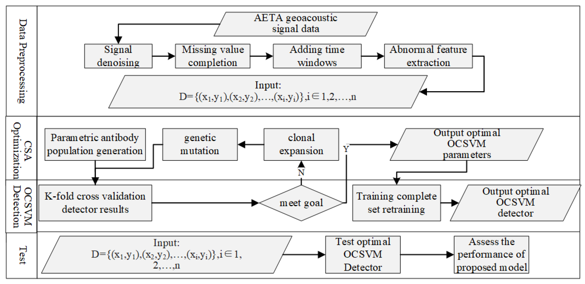
To effectively solve the problem of geoacoustic anomaly detection, the proposed geoacoustic anomaly detection model based on the CSA-OCSVM algorithm is described in Figure 2; it includes three parts: the data preprocessing stage, training process (including OCSVM detection, CSA parameter adjustment process), and testing process. Firstly, the geoacoustic signal data, which are collected and stored in the AETA system, serve as the original data. To solve the problems of noise and missingness in the original signal, processes such as signal denoising, missing value completion, time window addition, and abnormal feature extraction are carried out. Then, the detector training phase involves obtaining the optimal OCSVM detector through the training of geoacoustic signal sample sets and continuous parameter adjustment using CSA. It is mainly divided into two parts: the OCSVM detection process and the CSA parameter adjustment process. Finally, the detection phase aims to implement the optimal OCSVM detector selected in the previous stage to process the test sample set and isolate abnormal data that does not meet the feature indicators of normal geoacoustic signal data in the sample set.

3.1. Acoustic Signal Processing

The data preprocessing work of this model is divided into four steps: signal denoising, missing value completion, adding time windows, and abnormal feature extraction. The goal is to process the input geoacoustic signal original data and obtain a set of geoacoustic signals that can represent the geoacoustic signal within a period of time.

Signal denoising: The boxplot method is used to remove sudden jump points in the denoising stage to process the original data of geoacoustic signals. Based on the characteristic differences between real geoacoustic anomalies and background interference noise, obvious sudden jumps are identified for point and outlier removal. When drawing the boxplot of the original geoacoustic signal data, first, the number axis is determined according to the magnitude of the data, and the samples in the dataset are arranged in ascending order. Assume the size of the dataset is n; then the sorted set is described as $T=\{x_1,x_2,\dots ,x_n\}$. The points corresponding to the maximum sample $x_n$ and the minimum sample $x_1$ are marked on the number axis, and then the sizes of the first quartile $Q1$, the median $Q2$, and the third quartile $Q3$ are calculated, respectively. In addition, the distance between the first quartile $Q1$ and the third quartile $Q3$ is called the IQR. The length of the IQR is then adopted as the width of the rectangle, to draw a rectangular box between $Q1$ and $Q3$, a line segment at the median $Q2$ to represent the data in the middle, and a line segment at $Q1-1.5IQR$ and $Q3+1.5IQR$, respectively. Finally, a line segment parallel to the median line should be drawn at each position to identify abnormal sample data.

Missing value completion: The cubic spline interpolation method originated from the spline curve used by graphics engineers. It is an algorithm that fits a smooth continuous function curve through a set of discrete point changes. Suppose the cubic spline interpolation function containing $n+1$ data points is $S\left(x\right)$, then it satisfies: (1) Let $S_i\left(x\right)$ be the expression on the ith monotonically increasing piecewise interval $[x_i,x_{i+1}]$ of $S\left(x\right)$, then $S_i\left(x\right)$ is a cubic polynomial; (2) $S\left(x_i\right)=y_i$; (3) $S\left(x\right)$ and its first and second derivatives are continuous within a limited interval; $S_i\left(x\right)$ can be described as shown in Equation (1),

$$S_i\left(x\right)=a_i+b_i\ast (x-x_i)+c_i\ast {(x-x_i)}^2+d_i\ast {(x-x_i)}^3,i=0,1,\dots ,n-1$$

(1)

where $a_i$, $b_i$, $c_i$, and $d_i$ represent the undetermined coefficients of the function, respectively. Taking into account the continuity of $S_i\left(x\right)$ and the continuity of its first-order derivative and second-order derivative, let the second-order derivative value at both ends of the curve be 0. By substituting $n+1$ data points into the solution, $S_i\left(x\right)$ is expressed as shown in Equation (2),

$$\begin{array}{c}{S}_i\left(x\right)=y_i+{\alpha }_i\ast (x-x_i)+m_i/2\ast {(x-x_i)}^2+(m_{i+1}-m_i)/6h_i\ast {(x-x_i)}^3,\\ {\alpha }_i=(y_{i+1}-y_i)/h_i-h_i\ast m_i/2-(m_{i+1}-m_i)/6\ast h_i\end{array}$$

(2)

where $h_i$ is the step value of $x_{i+1}-x_i$, and $m_i$ is the second derivative value at $x_i$. Through this interpolation calculation method, it is easy to complete the missing geoacoustic signal data to ensure the subsequent work of this model.

Adding time windows: After the above processes of denoising and interpolation, relatively complete and continuous geoacoustic signal time series data can be obtained, where each piece of data contains three characteristics: amplitude mean, ringing count, and peak frequency. When analyzing anomaly detection in time series data, it is usually necessary to use a time window to divide the time series data into a set of shorter sequences, and analyze whether there are abnormalities in the overall time series data through the characteristics of each sequence. After windowing processing, the original time series data containing 3-dimensional features are converted into a $3\times m$ data matrix X due to the size of the m time window, which can be described as shown in Equation (3).

$$X=\left[\begin{array}{ccc}{x}_{1,1}& \cdots & x_{m,1}\\ x_{1,2}& \cdots & x_{m,2}\\ x_{1,3}& \cdots & x_{m,3}\end{array}\right]$$

(3)

Abnormal feature extraction: The geoacoustic signal data matrix obtained through the above operations cannot be directly used as the input of the anomaly detection algorithm. It is also necessary to extract abnormal features, i.e., to extract those indicators that can better reflect the geoacoustic signal anomalies. Through preliminary analysis and experiments on geoacoustic signal data, this model extracts five geoacoustic anomaly characteristic indicators: characteristic function peak value ($F_{max}$), amplitude standard deviation (${\sigma }_A$), very poor amplitude ($R_A$), sum of ring counts ($S_{rdc}$), and peak frequency ($P_f$). The calculation methods of these indicators are described in

Table 1. Signal weight values.

Indicators	Indicators
$F_{max}$	$max(x_{i+1}^2+((x_{i+1}-x_i)\ast {\sum }_{i=1}^l|x_i/x_i^{{}^{\prime }}{\left|\right)}^2)$
${\sigma }_A$	$\sqrt{{\sum }_{i=1}^n{(x_i-\overline{x})}^2/n}$
$R_A$	$x_{max}-x_{min}$
$S_{rdc}$	${\sum }_{i=1}^n{r}_i$
$P_f$	$f_{max}$

.

3.2. CSA-Based OCSVM

The detector training phase, named CSA-based OCSVM, aims to obtain the optimal OCSVM detector through continuous training of the training sample set and continuous parameter optimization of CSA, which can more effectively detect geoacoustic signal anomalies based on the extracted feature indicators. The main process is shown in Figure 3, which mainly includes the OCSVM detection process and the CSA parameter adjustment process.

The OCSVM detection process aims to verify the validity of the parameters provided by the CSA algorithm, which is executed cyclically in this algorithm model until it reaches the detection effect threshold or iteration number threshold. The main input data of this process include the geoacoustic signal data feature set subset D obtained in the data preprocessing stage, the penalty factor C given by the CSA algorithm, and the RBF kernel function parameter K. The target output is the best value after the CSA parameter adjustment optimization and the optimal OCSVM detector.

The feature set D in the input data can be directly processed using the OCSVM decision function, and its form can be described as shown in Equation (4),

$$y=sgn[\sum _{i=1}^l{\alpha }_{i}K(x_i,x)-\rho ],0\le {\alpha }_i\le C,\sum _{i=1}^l{\alpha }_i=1$$

(4)

where $K(x_i,x)$ adopts the RBF kernel function; therefore, y can be described as shown in Equation (5).

$$y=sgn[\sum _{i=1}^l{\alpha }_{i}exp(-\parallel x_i{-x\parallel }^2/2{\sigma }^2)-\rho ]$$

(5)

Then, the OCSVM discriminant function that can be used for anomaly detection can be obtained. To reduce the model detection error, the K-fold cross-validation method is used to divide the original training set into K equal parts, so each part is used as a set of test sets, and the remaining $K-1$ parts are used as the training set. Thus, K training models are obtained, and then the average detection accuracy of these models is used as the detection effect score of the OCSVM model under this parameter. In addition, when the detection effect of OCSVM reaches the expected threshold, i.e., when the CSA parameter optimization is completed and the optimal parameters are obtained, the parameters at this time need to be used to detect the entire training set to obtain the optimal OCSVM detector.

The input data of the CSA parameter adjustment process are mainly the maximum evolution algebra $maxgen$ and mutation probability p of the parameters related to the CSA algorithm. The former is used to ensure the convergence of the algorithm model to avoid falling into an infinite loop process due to the failure of finding the optimal solution, and the latter is used to control the mutation probability of each gene in the antibody. The output data of this process are the optimal parameters of OCSVM after parameter adjustment, including penalty factor C and the RBF kernel function parameter, $\sigma$. The entire parameter adjustment process can be divided into four key steps: antibody population generation, affinity calculation, clonal amplification, and genetic mutation.

Antibody population generation: The antibodies in this model correspond to the feasible C and $\sigma$ parameter values of OCSVM. Based on literature experience and preliminary experimental exploration, the value ranges are controlled at [0.5, 127.5] and [0.7, 178.5], respectively. The two parameters are compiled into a total of 16-bit antibody genes in binary form, where the first 8 bits represent C and the last 8 bits represent $\sigma$. The initial antibody population is then composed of 20 machine-generated antibodies.

Calculate affinity: In this model, the affinity between the antibody and the target antigen is measured by the detection accuracy score obtained during the OCSVM detection process. When the affinity of the existing antibody reaches the threshold, i.e., the detection effect score reaches the expected value or the current evolution generation reaches the maximum evolution generation $maxgen$, CSA adjusts the parameters. The process ends and the current C and $\sigma$ are output.

Clone expansion: Clonal expansion determines the number of species based on the affinity of individuals in the antibody population through a quantitative process. Arrange the various antibody types in the population according to their affinity. The total number of new clones of each type of antibody, $N_{clone}$, can be described as shown in Equation (6),

$$N_{clone}=\sum _{i=1}^{n}round(\lambda N_i/i)$$

(6)

where $\lambda$ represents the clone amplification multiple, i represents the ranking of the current antibody type in the affinity order, and $N_i$ represents the number of previous antibody clones at position i.

Genetic mutation: According to the inverse relationship between the antibody affinity and mutation rate, mutation operations are performed on individuals in the antibody population. The mutation rate $p_i$ of each antibody type in the affinity order can be described as shown in Equation (7),

$$p_i=p/(n+1-i)$$

(7)

where the current antibody with the highest affinity remains unchanged. The specific mutation operation involves randomly selecting the 16$p_i$ gene from the i-th antibody for mutation. Since it is binary coded, the mutation operation for the j-th gene $g_j$ of a certain antibody can be described as $g_j=|1-g_j|$.

To summarize, the pseudocode of CSA-OCSVM is depicted as Algorithm 1.

Algorithm 1 CSA-OCSVM

Input: Geoacoustic signal characteristic index dataset D, maximum number of iterations $maxgen$, mutation probability p, clone amplification multiple $\lambda$, deletion ratio $r_{del}$, detection accuracy expectation threshold $\phi$. Output: Abnormal label. Randomly generate 20 non-repeating random antibodies as the initial antibody population P; $gen\leftarrow 0$; $max\_aff\leftarrow 0$; while true do    for Each antibody in P do      $C\leftarrow bit2num$(first eight digits of antibodies) ∗ 0.5, $C\in [0.5,127.5]$;      $\sigma \leftarrow bit2num$(last eight digits of antibodies) ∗ 0.7, $\sigma \in [0.7,178.5]$;      Divide D into abnormal sample set E and normal sample set N;      Divide N into 5 disjoint subsets $\{N_1,N_2,\dots ,N_5\}$/;      for Each subset $N_i$ of N do         Use this subset together with the random half of the data in E as the test set T; the other 4 subsets are the training set S;         Set C as the penalty factor and $\sigma$ as the kernel parameter of the RBF kernel function;         $model\leftarrow ocsvm\_train(C,\sigma ,S)$;         Mark abnormal $T\leftarrow ocsvm\_test(model,T)$;         Calculate TPR;      end for      $anti\_aff\leftarrow$ 5 times the average TPR as antigen affinity;    end for    Sort the antibodies in P in descending order by $anti\_aff$;    Delete the antibodies with the lowest affinity ($r_{del}$*number of antibodies);    $max\_aff\leftarrow max(anti\_aff)$;    for $gen>maxgen$ do      if $gen>maxgenand\phi >max\_aff$ then         break;      end if    end for    for each antigen type in P do      $n\leftarrow round(\lambda \ast$ the number of previous types/the affinity order of this type of antibody);      Copy n copies of this antibody;    end for    for each antigen in P do      if $anti\_aff==max\_aff$ then         continue;      end if      Random mutations in anti $16\ast p/(totalnumberofantibodies+1-affinityorder)$ genes;    end for    $gen\leftarrow gen+1$; end while Divide D into a training set S and a test set T, where all abnormal samples are put into T; Set C as the penalty factor and $\sigma$ as the kernel parameter of the RBF kernel function; $model\leftarrow ocsvm\_train(C,\sigma ,S)$; Label abnormal signals $T\leftarrow ocsvm\_test(model,T)$.

3.3. Detection and Assessment

The detection stage mainly uses the optimal OCSVM detector selected in the previous stage to process the test sample set, isolate abnormal data that do not meet the characteristic indicators of normal geoacoustic signal data in the sample set, and evaluate its abnormal detection results. The core issue at this stage is how to evaluate the effectiveness of the anomaly detection algorithm model. Since anomaly detection problems usually have the characteristic of an imbalance between positive and negative samples, the effect of anomaly detection cannot simply be evaluated by the ratio of identified normal samples to the total samples. Instead, the TPR and FPR should be used to evaluate the quality of the anomaly detection algorithm.

The TPR refers to the ratio of positive samples judged as positive by the algorithm model to the total number of actual positive samples. In the geoacoustic signal anomaly detection experiment, i.e., the ratio of the detected normal geoacoustic signal data to the total number of actual normal geoacoustic signals. TPR can be described as shown in Equation (8).

$$\mathrm{TPR}=\mathrm{TP}/\mathrm{TP}+\mathrm{FN}$$

(8)

In the same way, FPR refers to the ratio of negative samples misjudged as positive by the algorithm model to the total number of actual negative samples, which can be described as shown in Equation (9).

$$\mathrm{FPR}=\mathrm{FP}/\mathrm{FP}+\mathrm{TN}$$

(9)

This study will use the above-mentioned two evaluation indicators, TPR and FPR, to evaluate the effect of the CSA-OCSVM algorithm model on geoacoustic signal anomaly detection.

3.4. Time Complexity Analysis

The time complexity of CSA-OCSVM is $O(ite\ast n^2)$, where $ite$ is the number of algorithm iterations, and n is the number of data instances. CSA-OCSVM updates the weights in OCSVM. The main time costs focus on the OCSVM anomaly detection and CSA optimization process. In the OCSVM anomaly detection process, the algorithm performs operations of signal fusion and classification. The time complexity of OCSVM is $O\left(n^2\right)$. With the optimization process, the algorithm uses the CSA to adjust the weight of OCSVM. The number of calculation times does not exceed the iteration numbers $ite$, and the time costs are $O\left(ite\right)$. Therefore, the total time complexity of the CSA-OCSVM is $O(ite\ast n^2)$.

4. Experimentation

In this section, the experiments are introduced in detail, and the results of the proposed CSA-OCSVM and baselines on AETA geoacoustic datasets are demonstrated. Through several experiments, we comprehensively analyze the performance of the proposed CSA-OCSVM. All approaches are run in Python 3.6 and implemented on a machine with an Intel Xeon E5-2640 v3 8-Core CPU. All the algorithms are verified by a ten-fold cross-validation method, and the mean and standard deviations of each evaluation indicator are reported.

4.1. Datasets

The geoacoustic signal data required for the experiment come from the AETA multi-component seismic monitoring system, which is shown in Figure 4. To reduce and avoid experimental bias caused by regional differences, 30 consecutive days of geoacoustic signal data from one observation station were selected in each of the eight provincial-level administrative regions, which were collected by various sensors we developed in AETA, i.e., Sichuan, Yunnan, Taiwan, Hebei, Guangdong, Qinghai, Jilin, and Beijing. Each observation station collected 144 data records every day. The original dataset contains a total of 34,560 geoacoustic signal data records. The specific observation stations and time selections are shown in

Table 2. AETA geoacoustic data information used in the experiment.

Station ID	Province	Location	Data Collection Time
48	Sichuan	(104.79, 28.38)	2021.02.20–2022.03.20
152	Yunnan	(100.59, 25.83)	2021.07.01–2022.07.30
79	Taiwan	(121.14, 24.71)	2021.01.31–2022.02.29
54	Hebei	(118.52, 39.13)	2021.12.01–2022.12.30
230	Guangdong	(113.91, 22.49)	2021.01.01–2022.01.30
227	Qinghai	(97.01, 33.01)	2021.03.01–2022.03.30
25	Jilin	(124.97, 45.42)	2021.06.01–2022.06.30
61	Beijing	(116.47, 39.68)	2021.12.01–2022.12.30

.

4.2. Data Preprocessing

The original data obtained from AETA require data preprocessing, including the following four steps: signal denoising, missing value completion, adding time windows, and abnormal feature extraction. The following phase uses the data from the Jinniu Town No. 2 Primary School Observation Station as an example to perform the preprocessing process of the original data of the geoacoustic signal. The original data are shown in

Table 3. AETA geoacoustic data information of the Jinniu Town No. 2 Primary School Observation Station.

ID	Data Collection Time	Amplitude Mean Value	Ring Count	Peak Frequency
1	190701	0.240109	0	146.48
2	190701	0.232378	0	146.48
3	190701	0.225153	0	146.48
4	190701	0.218461	0	146.48
5	190701	0.213167	0	146.48
6	190701	0.204784	0	146.48
7	190701	0.195161	0	146.48
…	…	…	…	…
4320	190730	0.137343	0	146.48

.

We should draw boxplots for the mean amplitude, ring count, and peak frequency in the original data of the low-frequency geoacoustic signal. Points outside the two line segments $Q1-1.5IQR$ and $Q3+1.5IQR$ in the figure are marked as suspected noise points. Then, only one of these suspected noise points is eliminated every 6 h. This approach minimizes noise interference caused by sudden jump points without significantly affecting the identification of earthquake-related abnormal signals. Missing values caused by equipment and the aforementioned denoising process were processed using cubic spline interpolation on a daily basis. Each day’s 144 pieces of data are numbered, and this serial number is used as shown in Figure 4.

For anomaly detection and analysis of time series data, it is usually necessary to use a time window to divide the time series data into a set of shorter sequences. This allows analysis of whether there are anomalies in the overall time series data through the characteristics of each sequence. Preliminary experiments have verified that when 6 h is used as the length of a single time window, the true rate of the anomaly detection experiment reaches a relatively good level. Therefore, the experiment chose to divide the geoacoustic signal time series data into 6-h units. After normalization processing, a geoacoustic signal characteristic index dataset suitable for experiments was finally obtained, including a total of 960 sets of data from eight provinces and regions, as shown in

Table 4. Geoacoustic signal characteristic index dataset.

Time	${\mathit{F}}_{\mathit{m}\mathit{a}\mathit{x}}$	${\mathit{\sigma }}_{\mathit{A}}$	${\mathit{R}}_{\mathit{A}}$	${\mathit{S}}_{\mathit{r}\mathit{d}\mathit{c}}$	${\mathit{P}}_{\mathit{f}}$	Label
19070100	0.0453372	0.0858874	0.0101610	0.0013145	0.0342165	0
19070106	0.0546628	0.0844023	0.0108135	0.0018013	0.0344271	0
19070112	0.0514571	0.0826160	0.0105247	0.0014241	0.0404989	0
19070118	0.0503421	0.0811309	0.0101752	0.0013210	0.0407094	0
…	…	…	…	…	…	…

.

4.3. The Prototype Implementation

The geoacoustic signal anomaly detection in our study is a binary classification task; therefore, we introduce the IQR [9], GA-OCSVM, and PSO-OCSVM [13] for comparison with our proposed CSA-OCSVM. The advantage of IQR is that it is not affected by the 25% values at both ends. It can measure the degree of difference in the open group sequence and measure the representativeness of the median. The disadvantage is that it cannot reflect the degree of difference of all flag values. The GA has good global search capabilities and can quickly search out all solutions in the solution space without falling into the trap of the rapid decline of local optimal solutions. However, the local search ability of the genetic algorithm is limited, which makes the simple genetic algorithm more time-consuming and results in lower search efficiency in the later stages of evolution. In practical applications, genetic algorithms are prone to premature convergence problems. The PSO algorithm has a fast convergence speed and is easy to program and implement. However, its accuracy is not high.

In our experiments, the input signals are normalized between 0 and 1. In GA-OCSVM, the initial C is set to 1, the initial population size is 20, the max evolutionary number is 100, the cross rate is 0.5, and the mutation rate is 0.005. For the PSO-OCSVM approach, the max iteration is 100 and the population size is 20. The acceleration coefficients $c_1$ and $c_2$ are 0.49 and 0.51, respectively. The inertia weight $\omega$ is 0.5. In CSA-OCSVM, the initial antigen population size is 20, the max iteration is 100, and the mutation rate is 0.5. Other parameter settings of the comparison methods can be found in the relevant literature.

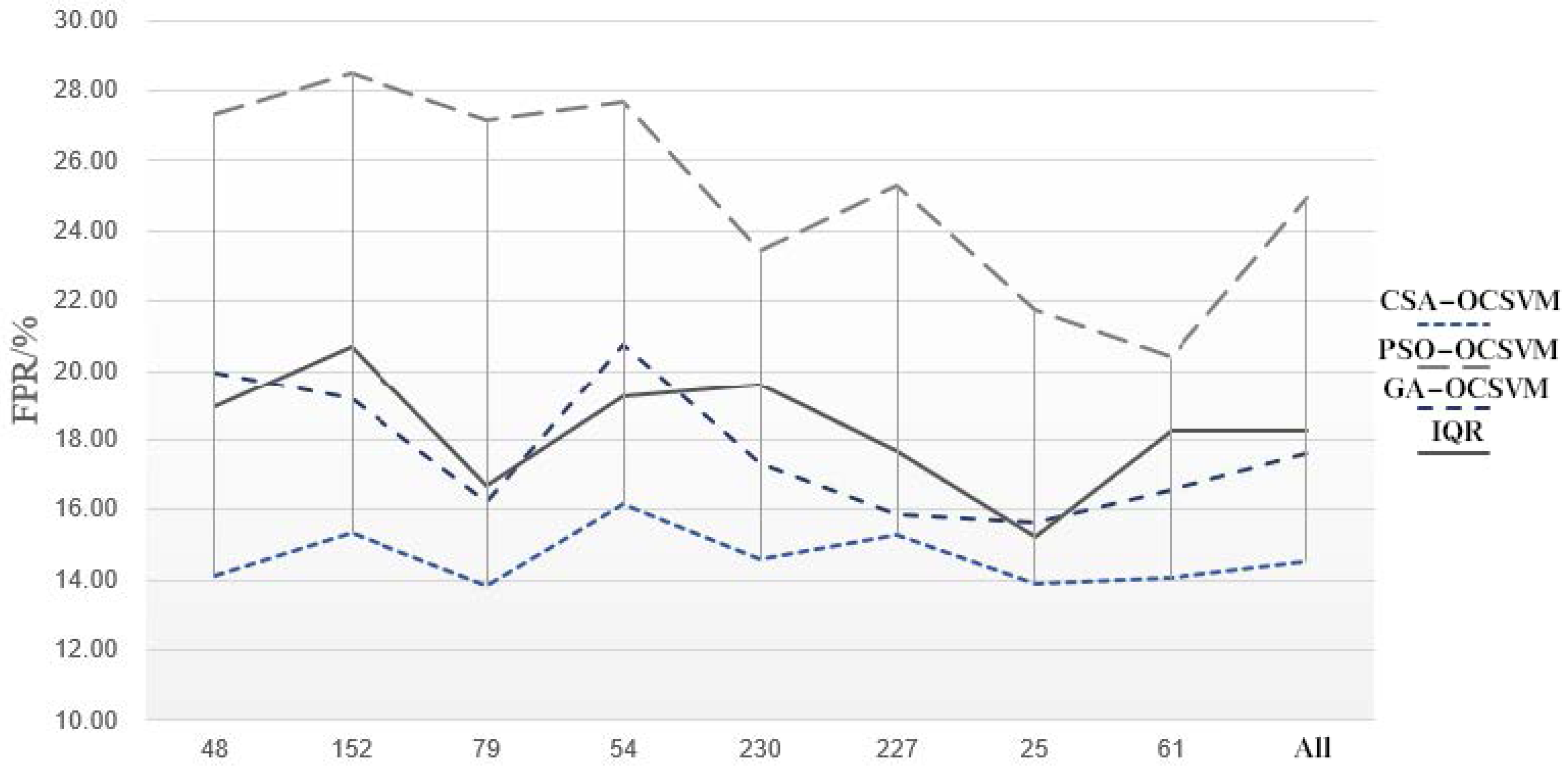
4.4. Results Analysis and Comparison

We conducted 10 anomaly detection experiments on 8 groups of datasets and the entire dataset using the experimental designs mentioned above, and recorded the average TPR and FPR of the 10 experiments. The experimental results are demonstrated in

Table 5. Comparison between CSA-OCSVM and other approaches with TPR, the best results are in bold.

Station ID	IQR	GA-OCSVM	PSO-OCSVM	CSA-OCSVM
48	89.94 ± 0.11	88.86 ± 0.12	84.59 ± 0.54	91.13 ± 0.01
152	85.40 ± 0.32	87.39 ± 0.65	82.42 ± 0.01	90.37 ± 0.16
79	85.15 ± 0.12	86.87 ± 0.73	79.80 ± 0.33	89.19 ± 0.21
54	87.85 ± 0.23	87.01 ± 0.11	81.31 ± 0.09	89.72 ± 0.01
230	87.23 ± 0.04	91.81 ± 0.15	83.19 ± 0.12	92.55 ± 0.00
227	86.41 ± 0.69	88.35 ± 0.54	82.52 ± 0.43	90.68 ± 0.01
25	86.60 ± 0.12	85.57 ± 0.17	84.85 ± 0.12	90.31 ± 0.03
61	83.40 ± 0.92	85.11 ± 0.21	82.23 ± 0.22	88.51 ± 0.12
All	86.49 ± 0.11	87.60 ± 0.11	82.57 ± 0.67	90.29 ± 0.12

and

Table 6. Comparison between CSA-OCSVM and other approaches with FPR, the best results are in bold.

Station ID	IQR	GA-OCSVM	PSO-OCSVM	CSA-OCSVM
48	18.97 ± 0.12	19.94 ± 0.09	27.33 ± 0.34	14.15 ± 0.00
152	20.73 ± 0.07	19.17 ± 0.23	28.50 ± 0.21	15.34 ± 0.12
79	16.67 ± 0.01	16.19 ± 0.34	27.14 ± 0.17	13.81 ± 0.23
54	19.23 ± 0.28	20.77 ± 0.12	27.69 ± 0.07	16.15 ± 0.01
230	19.62 ± 0.19	17.31 ± 0.50	23.46 ± 0.32	14.62 ± 0.11
227	17.65 ± 0.09	15.88 ± 0.19	25.29 ± 0.47	15.29 ± 0.09
25	15.22 ± 0.31	15.65 ± 0.20	21.74 ± 0.32	13.91 ± 0.01
61	18.23 ± 0.38	16.54 ± 0.17	20.38 ± 0.12	14.04 ± 0.00
All	18.28 ± 0.17	17.63 ± 0.06	24.94 ± 0.06	14.52 ± 0.22

and Figure 5. Therefore, a more intuitive comparison chart of TPR and FPR in the experimental scenarios can be drawn, as shown in Figure 6 and Figure 7.

Based on the above experimental results, the following conclusions can be drawn.

• There is an obvious difference in the experimental results between CSA-OCSVM and PSO-OCSVM. The detection results in PSO-OCSVM are poor, and the FPR is high. This is because CSA has the advantages of global optimization, dynamic adaptation, and parallel search and, therefore, can obtain more suitable hyperparameters for OCSVM.
• From the comparison of the experimental results of CSA-OCSVM and GA-OCSVM, it can be seen that when the maximum number of iterations is the same, the OCSVM anomaly detector is more likely to reach the optimum under the optimization of the CSA than under the optimization of the GA. This verifies the effectiveness of the CSA for OCSVM algorithm optimization.
• From the comparison of the experimental results of CSA-OCSVM and IQR, it can be seen that the anomaly detection effect of the model proposed in this study on the geoacoustic signal data in the AETA system can reach or even surpass the more mature sliding quartile method based on Baer features, which verifies the effectiveness of the geoacoustic signal anomaly detection model based on the CSA-OCSVM algorithm. In addition, according to the comparison between GA-OCSVM and IQR, it can also be found that when the CSVM parameters are not adjusted to an optimal level, the performance of the IQR method may be better than the OCSVM algorithm.
• In addition, in other experiments on earthquake precursor data anomaly detection [26], FPR was basically controlled below 10%. The FPR obtained from the four experimental scenarios in this study are all on the high side, indicating that the FPR of the anomaly detection experiment is high. The reason for this problem may be the low signal-to-noise ratio of the geoacoustic signal data. Although the data preprocessing stage, to a certain extent, reduces the interference of noise fluctuations on the results, limitations in our research level and research time mean there are still larger problems in this regard.

In summary, the geoacoustic anomaly detection model based on the CSA-OCSVM algorithm proposed in this paper can achieve satisfied anomaly detection results for low-frequency geoacoustic data in the AETA system.

4.5. Ablation Studies

In this study, CSA has an advantage in optimizing the parameters of a classification algorithm. Therefore, we introduce it into the optimization of OCSVM, and to verify its impact on the OCSVM, the accuracy results of OCSVM and CSA-NF-OCSCM are compared and analyzed on the above-mentioned nine datasets. CSA-NF-OCSCM is a model without the $F_{max}$ indicator. The CSA layer is combined with the OCSVM layer. For each sample, the CSA layer acquires normalized data from the input instance and is realized by a CSA process. The CSA-OCSVM is implemented according to the indicator $F_{max}$ module and CSA, with the $F_{max}$ indicator adopted to improve the performance of the AMM.

As shown in

Table 7. The results of ACC for ablation studies, the best results are in bold.

Station ID	OCSVM	CSA-NF-OCSVM	CSA-OCSVM
48	83.51 ± 0.11	88.45 ± 0.09	90.89 ± 0.00
152	81.65 ± 0.21	86.12 ± 0.11	91.12 ± 0.10
79	80.21 ± 0.34	83.87 ± 0.43	88.76 ± 0.11
54	80.98 ± 0.10	86.34 ± 0.23	90.12 ± 0.09
230	82.21 ± 0.09	88.13 ± 0.11	91.98 ± 0.03
227	81.67 ± 0.23	85.91 ± 0.07	90.11 ± 0.00
25	83.79 ± 0.10	85.89 ± 0.09	90.54 ± 0.01
61	81.98 ± 0.11	82.87 ± 0.12	89.12 ± 0.12
All	82.11 ± 0.07	84.12 ± 0.10	89.33 ± 0.10

, the layer-by-layer performance analysis shows that the performance improved to a certain extent after adding the $F_{max}$. The results of the ablation studies indicate that the $F_{max}$ indicator and the CSA adjustment of parameters have a significant influence on the OCSVM. Generally, our proposed $F_{max}$ indicator and the CSA optimization mechanism in this study are key components for improving the performance of the OCSVM. This is because scenario one uses the characteristic index $F_{max}$, which can better amplify the energy fluctuations and amplitude abnormalities of the geoacoustic signal. Experimental results show that after using the $F_{max}$ index, the detector is less affected by noise and can significantly reduce the FAR, verifying the effectiveness of the feature extraction scheme in the model data preprocessing stage.

5. Conclusions and Future Work

This paper demonstrates a geoacoustic anomaly detection approach by integrating feature extraction strategies, OCSVM, and CSA. The main contribution of this paper is that it presents a novel CSA-OCSVM method to create a more suitable geoacoustic anomaly detection model. First, a data preprocessing scheme is designed to amplify the geoacoustic signal intensity and energy change rules, thereby reducing the interference of geoacoustic signal noise and intensity. Meanwhile, OCSVM is introduced for anomaly detection to address the imbalance of positive and negative samples in geoacoustic anomaly detection. Furthermore, in view of the optimization capabilities of the CSA, it is introduced to optimize the hyperparameters of OCSVM to improve its detection accuracy. Finally, the proposed approach is implemented for geoacoustic data anomaly detection in our self-developed AETA system to verify its effectiveness. The experimental results demonstrate that our proposed CSA-OCSVM is superior to the compared approaches.

In this study, the used CSA is derived from the function of B cells in the immune system. Unlike traditional geoacoustic signals anomaly detection methods, which lack adaptability, the proposed approach implements change adjustments based on the input sample. Meanwhile, the OCSVM can handle imbalanced samples, and the $F_{max}$ denotes the most significant geoacoustic signal. Moreover, with our self-collected geoacoustic signals by AETA, the real-world datasets have stronger credibility.

However, this study only focuses on the geoacoustic signals from AETA, neglecting other observed data, which are also important for earthquake prediction. Therefore, we will adopt other observed data with many more instances as our experimental data in future research. Moreover, future work will focus on enriching CSA and applying it to other earthquake-prone areas. We will further test CSA to improve other methods’ detection performance through subsequent experiments.