INNT: Restricting Activation Distance to Enhance Consistency of Visual Interpretation in Neighborhood Noise Training

Abstract

In this paper, we propose an end-to-end interpretable neighborhood noise training framework (INNT) to address the issue of inconsistent interpretations between clean and noisy samples in noise training. Noise training conventionally involves incorporating noisy samples into the training set, followed by generalization training. However, visual interpretations suggest that models may be learning the noise distribution rather than the desired robust target features. To mitigate this problem, we reformulate the noise training objective to minimize the visual interpretation consistency of images in the sample neighborhood. We design a noise activation distance constraint regularization term to enforce the similarity of high-level feature maps between clean and noisy samples. Additionally, we enhance the structure of noise training by iteratively resampling noise to more accurately depict the sample neighborhood. Furthermore, neighborhood noise is introduced to achieve more intuitive sample neighborhood sampling. Finally, we conducted qualitative and quantitative tests on different CNN architectures and public datasets. The results indicate that INNT leads to a more consistent decision rationale and balances the accuracy between noisy and clean samples.

1. Introduction

In recent years, deep convolutional neural networks have demonstrated superior performance compared to humans in various complex visual cognition tasks. However, when facing distribution shifts between training and application scenarios, deep convolutional neural networks can be easily disrupted by imperceptible input perturbations that are difficult for humans to notice [1,2]. For example, compression-induced artifacts on input images, which are visually imperceptible, can significantly reduce the accuracy of the model. A common approach is to introduce target noise into the training data, known as noise training, to learn task objectives with noise distributions during the training process. This enhances the model’s performance on noisy samples while generalizing the decision boundary of the model. Unfortunately, the generalization of the model’s decision boundary often does damage to the model’s decision performance, Dimitris et al. [3] demonstrated the inevitability.

Another critical issue in deep convolutional neural networks is interpretability. The black-box nature of the network renders the decision-making process opaque. There have been many studies on the interpretability of deep convolutional neural networks in different tasks. However, to the best of our knowledge, there has been limited research on the interpretability of noise training processes. This constitutes one of the primary motivations behind our work. We approach the interpretability of noise training from a simplistic perspective. When faced with similar clean and noisy samples, an ideal noise training process should ensure that the model not only makes correct classifications but also employs the same decision criteria. In reality, however, maintaining consistency in interpretability between clean and noisy samples in noise training proves to be a challenge. In light of this, we posit a hypothesis that noise training, while generalizing decision boundaries, erroneously introduces some easily overlooked interpretability loss, leading to an incorrect widening of decision boundaries in certain directions. Building upon this hypothesis, the performance loss incurred by generalized decision boundaries can be decomposed into generalization loss, which arises from the re-fitting after data distribution shifts and is theoretically unavoidable, and interpretability loss, which stems from overfitting to the noise distribution during the training process. The latter can induce the model to employ incorrect decision criteria for samples that have only minute amounts of noise added.

The research in this paper aims to reduce this interpretability loss and proposes an end-to-end training framework called Interpretable Neighborhood Noise Training (INNT), which uses a regular term to constrain the generalization direction of the decision boundary, allowing the decision boundary of the deep neural network to expand in a reliable manner within the neighborhood of the input image. Our work takes a new perspective on the interpretability of noise training through visual interpretability. Simultaneously, we propose effective methods for interpretable noise training, which substantially enhance the noise training process of convolutional neural networks. This provides a more trustworthy pathway for decision generalization in object recognition tasks. This work provides the following contributions:

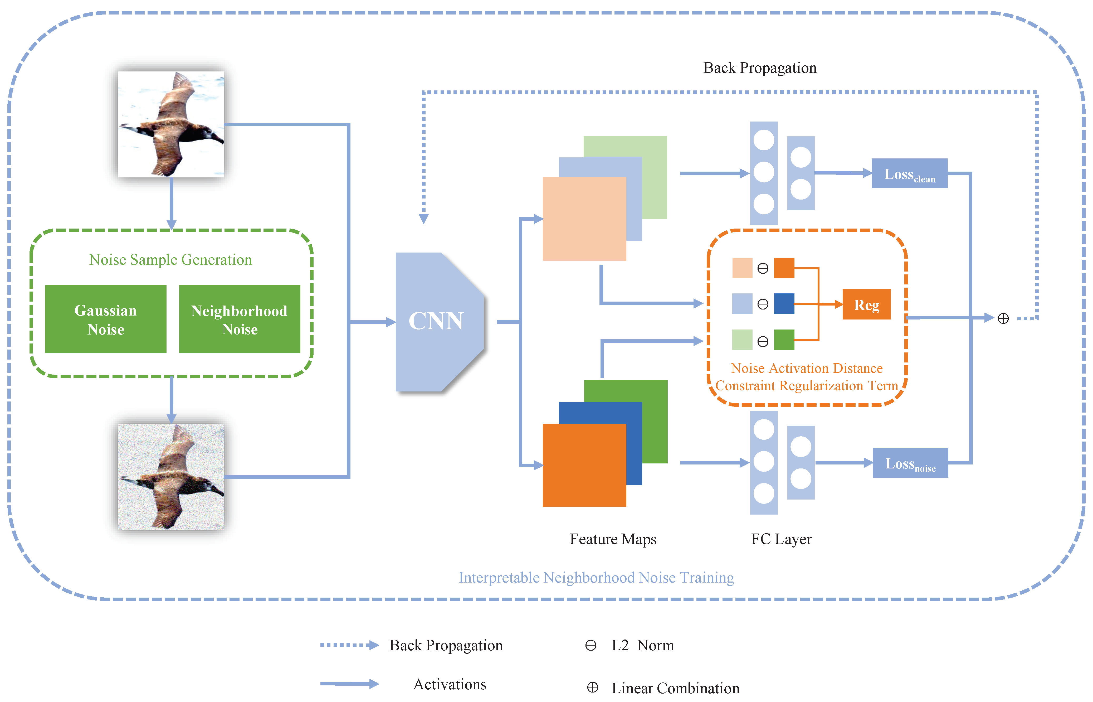
• We introduce an end-to-end framework called Interpretable Neighborhood Noise Training (INNT), along with a noise activation distance-constrained regularization term. For specific types of noise, this enables visually interpretable noise training, and it can be broadly applied to common deep convolutional neural network architectures.
• We propose neighborhood noise, a method for generating image noise by uniformly sampling tiny neighborhoods around each pixel. This approach allows generate visually similar noise images in a more controlled manner. And it can more effectively represent the approximate neighborhoods of the images.
• We applied Interpretable Neighborhood Noise Training (INNT) to AlexNet, VGG16, and ResNet, validating the effectiveness of INNT on the CUB-200-2011 and CIFAR-10 datasets. Our method demonstrated superior visual interpretability consistency and achieved closer predictive accuracy on similar images.

This paper is structured as follows: Section 1 provides an introduction, Section 2 discusses related work, Section 3 details the Interpretable Neighborhood Noise Training process, Section 4 presents qualitative and quantitative analysis of the experimental results, and finally, we conclude and suggest future work.

2. Related Works

2.1. Image Corruption

Image perturbation can be divided into common corruption and adversarial perturbation [4]. Common corruptions include a range of image distortions. Some studies have shown the vulnerability of deep convolutional neural networks to image perturbation. For example, Dodge and Karam [5] rigorously analyzed the impact of Gaussian noise, compression, contrast, and other image perturbations on the accuracy of CNNs in classification tasks. Geirhos et al. [6] compared additive noise effects on convolutional neural networks and human performance, and found that the classification patterns of DNNs are different from humans. Fine-tuning for a specific type of corruption does not have universality. Dan Hendrycks et al. [7] established the IMAGENET-P benchmark dataset for common corruptions and also discovered that adversarial defenses provide substantial robustness against common corruptions. Similar common corruption datasets include COCO-C, Pascal-C, Cityscapes-C [8], and MNIST-C [9]. Our noise function design takes into account the effectiveness of various common corruptions mentioned above, and references the design ideas of corruption datasets.

Another type of image perturbation that is widely studied is adversarial perturbation, which can specifically attack certain networks. Goodfellow et al. [2] proposed the FGSM algorithm, which assigns perturbation to the image by computing the gradient sign of the model’s loss function to minimize the loss function of the classification model. Dezfooli et al. [10] proposed the DeepFool algorithm, which calculates the minimum distance between the sample and the decision boundary at each iteration and moves the sample to the boundary, thus deceiving the model. Rony et al. [11] proposed a white-box attack algorithm to generate minimally perturbed adversarial examples based on Augmented Lagrangian principles. In addition to adding extra information to clean images, Duan et al. [12] used DCT transformation to reduce the high-frequency components in images and construct adversarial examples, opening up a new path for evaluating the frequency domain robustness of DNNs. Overall, adversarial perturbation is an extreme case of image perturbation, and we hope to extend INNT to defense against adversarial perturbation in future work.

2.2. Robustness Enhancements

There have been many attempts to enhance the robustness of DCNN (deep convolutional neural network) against common perturbations [13,14,15]. Xie et al. [16] used self-training to repeatedly expand the training set and improve the model’s robustness, reducing the average flip rate of ImageNet-P from 27.8% to 12.2%. Zhang [17] integrated anti-aliasing techniques from signal processing into VGG and ResNet to maintain shift equivariance, resulting in improved robustness against noise, blur, and scaling perturbations. Schneider et al. [18] observed that the distribution shift of image perturbations is reflected in the differences of the first and second moments of internal representations in DCNNs. They strengthened this distribution shift by estimating the Batch Normalization (BN) statistics of corrupted images. Pang et al. [19] re-examined the definition of robustness, arguing that the improper robust error defined by the loss function leads to excessive local smoothness. They proposed a robust error called SCORE to balance accuracy and robustness.

One popular approach to enhancing robustness is data augmentation, which involves applying random transformations to the training set [20]. Related research can be traced back to 1995 when M. Bishop [21] demonstrated that adding noise during the model training process is equivalent to adding a regularization term, which can enhance the model’s robustness and generalization ability. Xie et al. [16] used self-training to repeatedly expand the training set, reducing the average flip rate of ImageNet-P from 27.8% to 12.2%. Ford et al. [22] added Gaussian noise of varying magnitudes uniformly to each image, improving the robustness of InceptionV3. A similar experiment was conducted by Rusak et al. [4], where Gaussian-augmented images and clean images were evenly distributed in each batch. Unfortunately, fine-tuning for one type of perturbation alone does not necessarily generalize to other perturbations [23]. In fact, our work builds upon the foundation laid by Ford et al. and Rusak et al., where we generate a Gaussian-augmented copy for each clean image in every batch.

2.3. CNN Visual Interpretation

The interpretability of DCNN is a key issue, and there are various approaches to obtaining explanations. For example, Zhang et al. [24] improved the interpretability of the model by embedding interpretable sub-layers within the network. C.-C. Jay Kuo [25] proposed a RECOS mathematical model to figure out the important role of nonlinear layers. Wachter et al. [26] constructed counterfactual examples to explain the decision process of the original examples. One of the simplest methods is to analyze the feature maps, such as using a multi-layer deconvolution network to synthesize image representations of feature activations [27], or using backpropagation to synthesize images that maximize the output of specific neurons [28]. These explanation methods have different applicability and costs, such as modifying the network structure or additional computational overhead. However, we need a low-cost and visually intuitive explanation algorithm to measure the interpretability loss of noise training.

Fortunately, Class Activation Maps (CAMs) meet our requirements. CAM [29] replaces the fully connected and softmax layers with Global Average Pooling (GAP) and calculates the class activation maps by weighting the feature maps with the weights of the output feature map. GradCAM [30] improves upon CAM by avoiding modifications to the network structure. GradCAM++ [31] improves the weight calculation process and can be used correctly for multi-task learning. Furthermore, ScoreCAM [32] alleviates the reliance on gradients by upsampling the feature maps, and LayerCAM [33] calculates separate weights for feature maps from different layers, resulting in more accurate heatmaps generated by different layers. In this paper, Class Activation Maps are not only used to analyze the interpretability loss in noise training, but also inspire the design of the explanation regularization term that constrains the distance of noise activations.

3. Methods

Noise training can often effectively improve the model’s recognition performance on noise images, but the alignment of visual interpretations between clean images and noise images is rarely considered. In this regard, we proposed a training framework called INNT, which can effectively improve the high-level activation consistency of convolutional neural networks on visually similar images and make certain trade-offs in recognition performance. This section provides a detailed introduction to the interpretable neighborhood noise training framework. Figure 1 presents an overview of our approach, which consists of three components: noise activation distance regularization term, noise sample generation, and interpretable neighborhood noise training. The noise activation distance regularization term enforces the network to maintain similar decisions within the neighborhood of input samples, which is our primary innovation (Section 3.2). The noise sample generation employs various noise functions to generate neighborhood samples with respect to the input samples (we detail the requirements of noise functions and propose a more controllable neighborhood noise in Section 3.3). Considering the above two components, we introduce interpretable neighborhood noise training, which utilizes the resampling of neighborhood samples to satisfy the noise activation distance regularization requirements on inputs while mitigating potential fitting risks (Section 3.4). For the sake of clarity, in Section 3.1, we first introduce the general form of noise training, along with the interpretability assessment method for the noise training process. Furthermore, we formalize the definitions of certain symbols.

3.1. Noise Training and Saliency Maps

3.1.1. Noise Training

Noise training is a frequently used data augmentation technique. Its common approach involves incorporating samples with specific noise into the training process to improve the model’s robustness against noise. Given a set of input images I, the corresponding noise dataset is represented as follows:

$$I_{noisy}=I_{clean}\cup \left\{\Phi \left(i\right)\right|i\in I_{sample}and{I}_{sample}\subseteq I_{clean}\}$$

(1)

where $I_{sample}$ is a subset of the input image set $I_{clean}$ and $\Phi (·)$ is a function that generates specific noise. Note that the construction of the noise dataset typically occurs before noise training and is performed only once. Let $\mathcal{D}$ be the data distribution over noisy input pairs $(x,y)$m where $x\in I_{noisy}$ and $y\in \{1,\dots ,k\}$. Noise training trains a classifier $f_{\theta }\left(x\right)$ parameterized by $\theta$ by minimizing the risk of the noise set $I_{noisy}$.

$$\underset{\theta }{\min }\underset{x,y\sim \mathcal{D}}{\mathbb{E}}\left[{\mathcal{L}}_{CE}(f_{\theta }\left(x\right),y)\right]$$

(2)

where ${\mathcal{L}}_{CE}(·)$ denotes the Cross-Entropy Loss Function.

3.1.2. Saliency Map

To faithfully assess the interpretability of the noise training, we introduced saliency map methods, with CAM being a representative example. CAM is commonly employed to scrutinize the visual interpretative capacity of black-box models. As an improved version of CAM, GradCAM can generate class activation maps for input images without modifying the network or retraining. To compute the GradCAM saliency map, the gradient weights ${\alpha }_k^c$ with respect to the target class c are calculated as follows:

$${\alpha }_k^c=\frac{1}{Z}\sum _i\sum _j\frac{\partial y^c}{\partial A_{ij}^k}$$

(3)

where $A_{ij}^k$ denotes the value at position $(i,j)$ in channel k, $y^c$ denotes the predicted score of the network for class c, and Z is the normalization constant that ensures the sum of gradient weights equals 1. Furthermore, the formula for GradCAM is as follows:

$$GradCAM(A,c)=ReLU\left(\sum _k{\alpha }_k^c{A}^k\right)$$

(4)

Here, A is usually the feature map output of the last convolutional layer, c denotes the target class, and ${\alpha }_i^c$ denotes the weights concerning $A^k$.

We use sensitivity maps generated by GradCAM to help evaluate the visual interpretability of the model on noisy samples and clean samples after noise training. Specifically, we extract the feature maps from the final convolutional layer of the model trained with noise, i.e., the input of the first fully connected layer in VGG-16 or the output of the last residual block in ResNet. Subsequently, we proceed to visualize these feature maps. We compare the activation differences between the feature maps generated from the input clean images and their corresponding noise image (details of obtaining the noise image are shown in Section 3.3). This serves as a measure of the visual interpretability achieved through noise training.

3.2. Noise Activation Distance Constraint Regularization Term

The noise activation distance constraint regularization term comes from a natural intuition; assuming a neural network is fine-tuned from a clean dataset to a noisy dataset under ideal conditions, it means that the neural network has correctly modeled the relevant features of the target task, and the classification process of the network on the noisy dataset should not be affected by the additive noise distribution. In this case, a clean sample and a sample with a small amount of noise should be consistently recognized by the neural network. In other words, when using an external interpreter to identify the decision factors, the results should be entirely consistent, and considering practical situations, the explanations of both should remain at a similar level. In fact, when we use GradCAM to examine the model trained with noise, only a few samples meet the above conditions, as shown in Figure 2.

For the above situation, one possible reason is that during the process of noise training, the neural network’s decision boundaries are over-generalized locally, as shown in Figure 3. In such cases, the neural network tends to learn compatibility with the noise rather than more robust feature representations. To address this, we propose a regularization term called Noise Activation Distance Constraint ($Re{g}_{na}$) to mitigate the excessive introduction of noise distribution during the noise training process.

$$\begin{array}{cc}Re{g}_{na}\hfill & =log({∥\Phi \left(I_{clean}\right)-\Phi \left(I_{noise}\right)∥}_2^{\tau }+1)\hfill \\ & =log({∥A_{I_{clean}}-A_{I_{noise}}∥}_2^{\tau }+1)\hfill \end{array}$$

(5)

Here, ${\parallel ·\parallel }_2$ denotes the L2 norm, $\tau$ is an influence factor, $\Phi (·)$ denotes the part before the linear layer of the convolutional neural network, and the corresponding A denotes the output of the last convolutional layer, consistent with the meaning in Section 3.1.2. The main purpose of $Re{g}_{na}$ is to minimize the distance between the high-level feature maps of clean and noise images, allowing the network to widen the decision boundary while avoiding overlearning noise feature representations. Maintaining the similarity of high-level feature maps can provide semantic consistency at the object or part level [34], which ensures better visual interpretation consistency in object detection tasks. We choose the L2 norm to ensure similarity between the two feature maps, rather than demanding an exact match like the L1 norm. Moreover, the influence factor $\tau$ and $log(·+1)$ are used to scale the size of the regularization term around the noise training loss, adjusting the tolerance for boundary generalization.

Note that the use of $Re{g}_{na}$ is very limited. Compared to other noise training methods, $Re{g}_{na}$ requires clean images and noise images to be closer. Excessive noise, for example, may cause the value of the regularization term to vary significantly between batches, making it challenging for the model to fit.

3.3. Noise Sample Generation

To avoid fitting difficulties caused by excessive noise, we require an effective and controllable noise generation function $\Phi (·)$. An ideal noise generation function should satisfy the following properties:

• The noise function $\Phi (·)$ is widely applicable and can represent common image corruptions or natural disturbances.
• The amplitude of the noise generated by the function $\Phi (·)$ is controlled by a limited number of adjustable parameters.
• The noise generated by the function $\Phi (·)$ can effectively interfere with the classification decisions of the image classification system while keeping the noise amplitude at a low level.

Taking consideration of the three properties mentioned above, we selected Gaussian noise as a representative of common image perturbations. In addition, we design neighborhood noise that satisfies these constraints as a supplement. This section will provide a detailed introduction to these two types of noise functions.

3.3.1. Gaussian Noise

Gaussian noise is a probabilistic distribution that follows a normal distribution. It often occurs in the process of digital image acquisition. Existing research has shown that Gaussian noise augmentation is an effective means of noise defense [35] which can regularize the decision boundary of classifiers. In this work, we use Gaussian noise as a noise sampling method to obtain noisy samples. For the standardized input image $I_{clean}\in {\mathbb{R}}^{m\times n}$, a noise matrix of the same size is sampled from a standard Gaussian distribution, as shown in Equation (6).

$$Nois{e}^G=\left[nois{e}_{ij}\right]\in {\mathbb{R}}^{m\times n},nois{e}_{ij}\sim \mathcal{N}(0,1)$$

(6)

The noise image is defined as a linear combination of the noise matrix $Nois{e}^G$ and the input image $I_{clean}$, as shown in Equation (7):

$$I_{noise}^G=I_{clean}+{\mu }^G\left[\max \left(I_{clean}\right)-\min \left(I_{clean}\right)\right]\times Nois{e}^G$$

(7)

Here, ${\mu }^G$ is the noise intensity parameter. More specifically, $\left[\max \left(I_{clean}\right)-\min \left(I_{clean}\right)\right]$ scales the noise matrix automatically to an appropriate range. It is important to note that considering Property 3 of the noise generation function, ${\mu }^G$ theoretically should be a relatively small value satisfying Property 3. We follow the parameter setting in [4], setting ${\mu }^G$ to 0.15 to avoid introducing additional learning parameters.

3.3.2. Neighborhood Noise

In this work, we propose a noise generation method called neighborhood noise, which can effectively generate noise that is adjacent to the input samples at the pixel level. Under the constraints of Property 2 and Property 3, we believe that an ideal noise generation function can produce images that can be easily recognized by humans. This means that the noise generation function can be seen as random sampling within a neighborhood of the original image, as shown in Figure 4. For implementation, we add pixel-level random noise and constrain the noise to a specific range to control the neighborhood radius.

For a standardized input image $I_{clean}\in {\mathbb{R}}^{m\times n}$, we first sample a noise matrix $Nois{e}^N$ of the same size from a standard uniform distribution as follows:

$$Nois{e}^N=\left[nois{e}_{ij}\right]\in {\mathbb{R}}^{m\times n},nois{e}_{ij}\sim \mathcal{V}(0,1)$$

(8)

The neighborhood noise is represented as random sampling at each pixel with a radius of ${\mu }^N$:

$$I_{noise}^N=I_{clean}\left[1+{\mu }^N(Nois{e}^N-0.5)/0.5\right]$$

(9)

Furthermore, when there exist specific upper and lower limits $(a,b)$ for a certain image corruption or natural disturbance function $noise\left(I_{clean}\right)$, i.e., $max\left(noise\left(I_{clean}\right)\right)<I_{clean}+b$ and $max\left(noise\left(I_{clean}\right)\right)>I_{clean}+a$, there exists a minimum noise radius $\phi$ such that $\phi \ge max(\overline{a},\overline{b})$. Then, the neighborhood noise $I_{noise}^N$, parameterized by ${\mu }^N\ge \phi$, can be viewed as an approximate set of various image corruptions and natural disturbances when the noise magnitude is small. This property ensures that neighborhood noise satisfies Property 1.

Compared to Gaussian noise, neighborhood noise has clear upper and lower limits in its form, which can intuitively reflect the neighborhood radius of noise sampling while maintaining its disruptive effect on the network.

3.4. Interpretable Neighborhood Noise Training

The basic form of noise training is described in Section 3.1.1, but noise training does not support the interpretable training method based on the noise activation distance constraint mentioned above. Therefore, we propose an interpretable neighborhood noise training framework, as shown in Figure 1. Interpretable neighborhood noise training involves executing the noise generation function on each mini-batch to generate noise images corresponding to the samples $I_{clean}^{batch}$. Subsequently, the classification loss $Los{s}_{clean}$ and the noise loss are simultaneously computed on each mini-batch. The noise training loss $Los{s}_{NT}$ is defined as the sum of these two components:

$$Los{s}_{clean}=CELoss(I_{clean}^{batch},y)$$

(10)

$$Los{s}_{noise}=CELoss(Noise\left(I_{clean}^{batch}\right),y)$$

(11)

$$Los{s}_{NT}=Los{s}_{clean}+Los{s}_{noise}$$

(12)

Here, $Noise(·)$ represents the Gaussian noise and domain noise generation function mentioned in Section 3.3. To improve the visual consistency between the noise samples and the clean samples, the noise activation distance constraint regularization term $Re{g}_{na}$ from Section 3.2 is incorporated into the loss computation process of each mini-batch. The final loss function, incorporating the noise activation distance constraint regularization term, is defined as follows:

$$Los{s}_{INNT}^{origin}=Los{s}_{clean}+Los{s}_{noise}+Re{g}_{na}$$

(13)

Due to the repetitive sampling of noise samples for the calculation of the noise activation distance constraint, optimizing the noise loss $Los{s}_{noise}$ can easily lead to a loss in classification accuracy. To address this, we utilize the Focal Loss to balance the weights between the noisy task and the original task. The overall loss function can be expressed as follows:

$$Los{s}_{INNT}=\lambda Los{s}_{clean}+(1-\lambda )Los{s}_{noise}+Re{g}_{na}$$

(14)

Here, $\lambda$ is the weight balancing parameter, with $\lambda \in (0,1)$. After computing $Los{s}_i$, the network parameters are updated through backpropagation. Please note that the generated noise samples are destroyed before the next mini-batch and do not cause excessive memory consumption. The interpretable neighborhood noise training, with its repetitive sampling of noise, can accurately describe the neighborhood of each sample and help identify more interpretable decision boundaries for generalization.

4. Experiments

4.1. Dataset

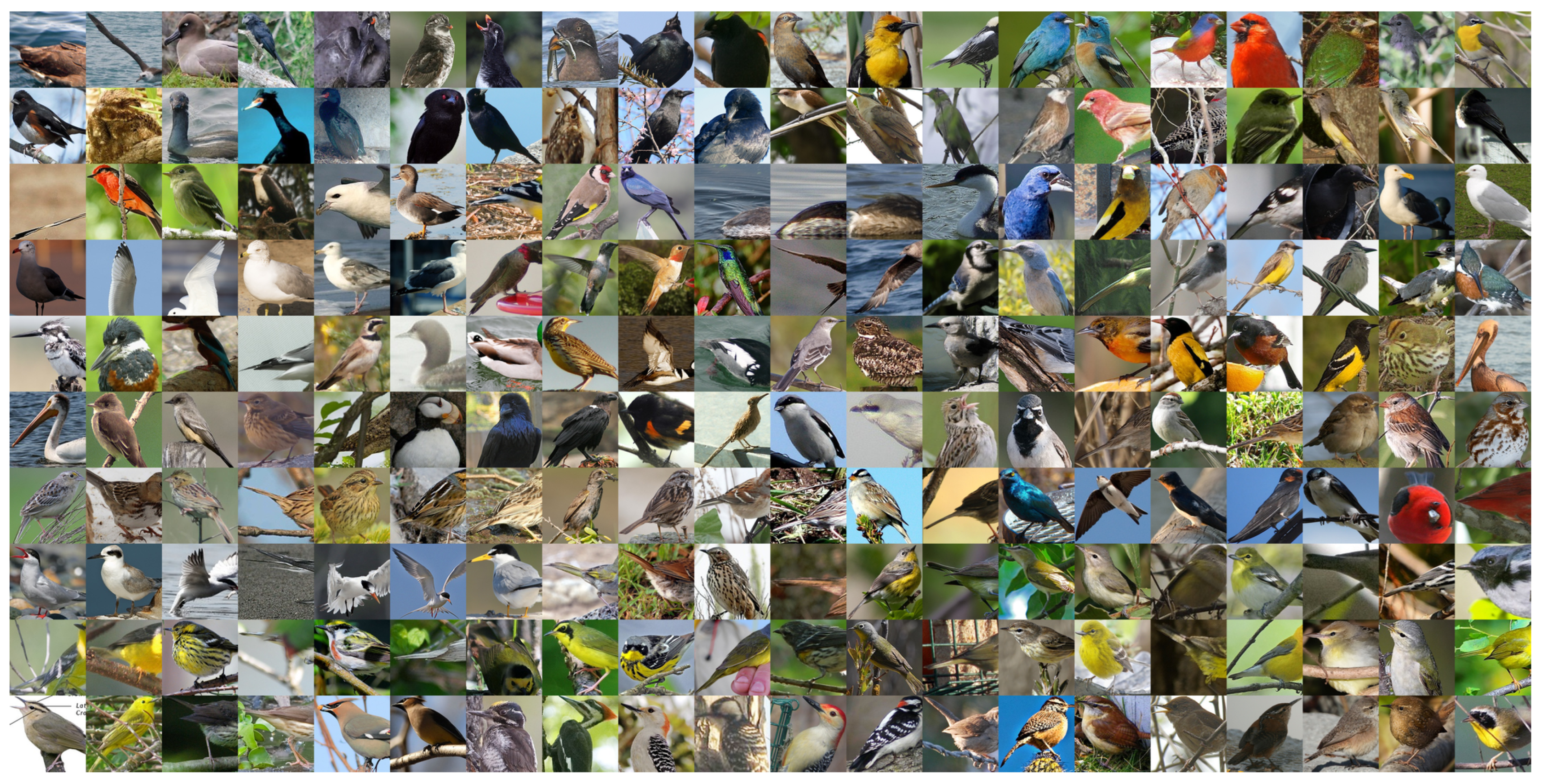
4.1.1. CUB-200-2011 Dataset

The Caltech-UCSD Birds-200-2011 (CUB-200-2011) dataset [36] is widely used for fine-grained visual categorization. It consists of 11,788 bird images divided into 200 subcategories, with 5994 for training and 5794 for testing, as shown in Figure 5. Each image has detailed annotations: 1 subcategory label, 15 part locations, 312 binary attributes, and 1 bounding box. During training, images are resized to 224 × 224 with random rotation and horizontal flip.

4.1.2. CIFAR-10

The research also utilized another dataset known as the CIFAR-10 dataset [37], short for the Canadian Institute for Advanced Research-10. CIFAR-10 serves as a benchmark dataset in the field of computer vision and is often used to evaluate the performance of deep learning models such as image classification and convolutional neural networks. CIFAR-10 comprises 60,000 images from ten mutually exclusive categories, including airplanes, automobiles, and birds. Each image in the CIFAR-10 dataset has dimensions of $32\times 32$. It is important to note that we did not modify the network architecture but instead resized the image dimensions to $224\times 224$, to match the configuration used for CUB-200-2011.

4.2. Implementation Details

All experiments were conducted on a single server, and the environmental configuration is outlined in

Table 1. Experiment environment.

Environment	Configuration
Operating System	Ubuntu 22.04
CPU	Intel(R) Xeon(R) Gold 6248R CPU @ 3.00GHz
GPU	NVIDIA RTX A6000 48GB
Memory	128GB
Python	3.9.13
Pytorch	1.13.0
CUDA	11.7

.

To assess the generalizability of our method, we selected three commonly used neural network architectures, namely AlexNet, VGG16, and ResNet18, as baselines. We loaded the corresponding pre-trained models, trained for 30 epochs with a batch size of 8. We recommend that the batch size be no larger than 16 to avoid excessive regularization penalties and ensure the stability of training. If a larger batch size is used, the feature map needs to be normalized, but this may affect the ability of the regularization term to align the activation of high-level neurons. All models were optimized using the Adam optimizer with default parameters. This choice facilitates rapid convergence and mitigates the potential impact of excessive hyperparameter tuning on the results. The remaining hyperparameters are detailed in

Table 2. Hyperparameters.

Hyperparameters	Value
$\tau$	$2\times {10}^{-3}$
$\lambda$	0.7
${\mu }^G$	0.15
${\mu }^N$	1.0

.

Here, $\tau$ and $\lambda$ are influenced by the introduced noise magnitude, which means their values are controlled by ${\mu }^G$ and ${\mu }^N$. In this study, we initially tested the interference capabilities of noise with different magnitudes on pre-trained models, as shown in Figure 6, and set ${\mu }^G$ to the most used value of 0.15. In this setting, the Top1 accuracy of VGG decreased to $14.26\%$. To maintain a similar level of accuracy loss, ${\mu }^N$ should have been set to 1.5, resulting in a Top1 accuracy of $13.24\%$. However, considering that the noise magnitude needs to be controlled to ensure the stability of $Re{g}_{na}$ during training, ${\mu }^N$ needs to be appropriately reduced. We observed in Figure 6 that the impact of neighborhood noise on the VGG network’s accuracy gradually decreases after ${\mu }^N>1.0$. Therefore, we set ${\mu }^N$ to 1.0 as a trade-off.

4.3. Evaluation Metrics

4.3.1. Faithfulness Evaluation via Image Recognition

The Average Increase and Average Drop metrics proposed in [31] are used to measure the faithfulness of class activation explanation maps in object recognition tasks. Rather than evaluating the faithfulness of the explanation algorithm itself, we measure the differences in faithfulness between class activation maps generated from clean images and noise images under the assumption of using the same explanation algorithm. These faithfulness differences serve as a measure of interpretability in the noise training process. Specifically, the Average Increase (AI) and Average Drop (AD) are defined in Equations (15) and (16).

$$\begin{array}{cc}\hfill AI& \hfill ={\sum }_{i=1}^N\frac{\max (0,Y_i^{c_{noise}}-Y_i^{c_{clean}})}{Y_i^{c_{cnoise}}N}\hfill \end{array}$$

(15)

$$\begin{array}{cc}\hfill AD& \hfill ={\sum }_{i=1}^N\frac{Sign(Y_i^{c_{noise}}<Y_i^{c_{clean}})}{N}\hfill \end{array}$$

(16)

where $Y_i^{c_{clean}}$ denotes the predicated score for class c on clean image $I_{clean}$, and $Y_i^{c_{noise}}$ denotes the predicated scores for class c when using the class activation maps of the noise image $I_{noise}$ as inputs, respectively. $Sign(·)$ denotes an indicator function that returns 1 if the input is true. A higher AI and a lower AD indicate that the predicted scores for noise images deviate less from the clean images, which means the model maintains a higher consistency between noisy and clean images. Keeping all other parameters of the model consistent implies that the noise training method has better interpretability.

4.3.2. Localization Evaluation

In this section, we evaluate the interpretability of the noise training process by measuring the localization capability. The Energy-based Pointing Game (EBPG) [32] is an energy-based metric used to evaluate localization capability. It measures the proportion of energy within the bounding box in the class activation map relative to the total energy, as defined in Equation (17).

$$\begin{array}{c}\hfill EBPG=\frac{\sum L_{(i,j)\in bbox}^c}{\sum L_{(i,j)\in bbox}^c+\sum L_{(i,j)\notin bbox}^c}\end{array}$$

(17)

We compute the EBPG separately on the class activation maps of clean images and noise images. The average error resulting from the EBPG on the CUB-200-2011 dataset serves as a metric to quantify the localization loss in noise training. We refer to this metric as the Average Energy-based Pointing Error (AEPE), defined as follows:

$$\begin{array}{c}\hfill AEPE=\frac{1}{N}{\sum }_{i=1}^N\left|EBP{G}_i^{clean}-EBP{G}_i^{noise}\right|\end{array}$$

(18)

In object recognition tasks, we aim for the model’s decision to consistently rely on the region of the image where the target object is located, regardless of the presence of noise. To evaluate this stability, we propose the AEPE, which characterizes the effectiveness of the explanation. A lower AEPE value indicates that the model is better equipped to maintain visual consistency across similar images.

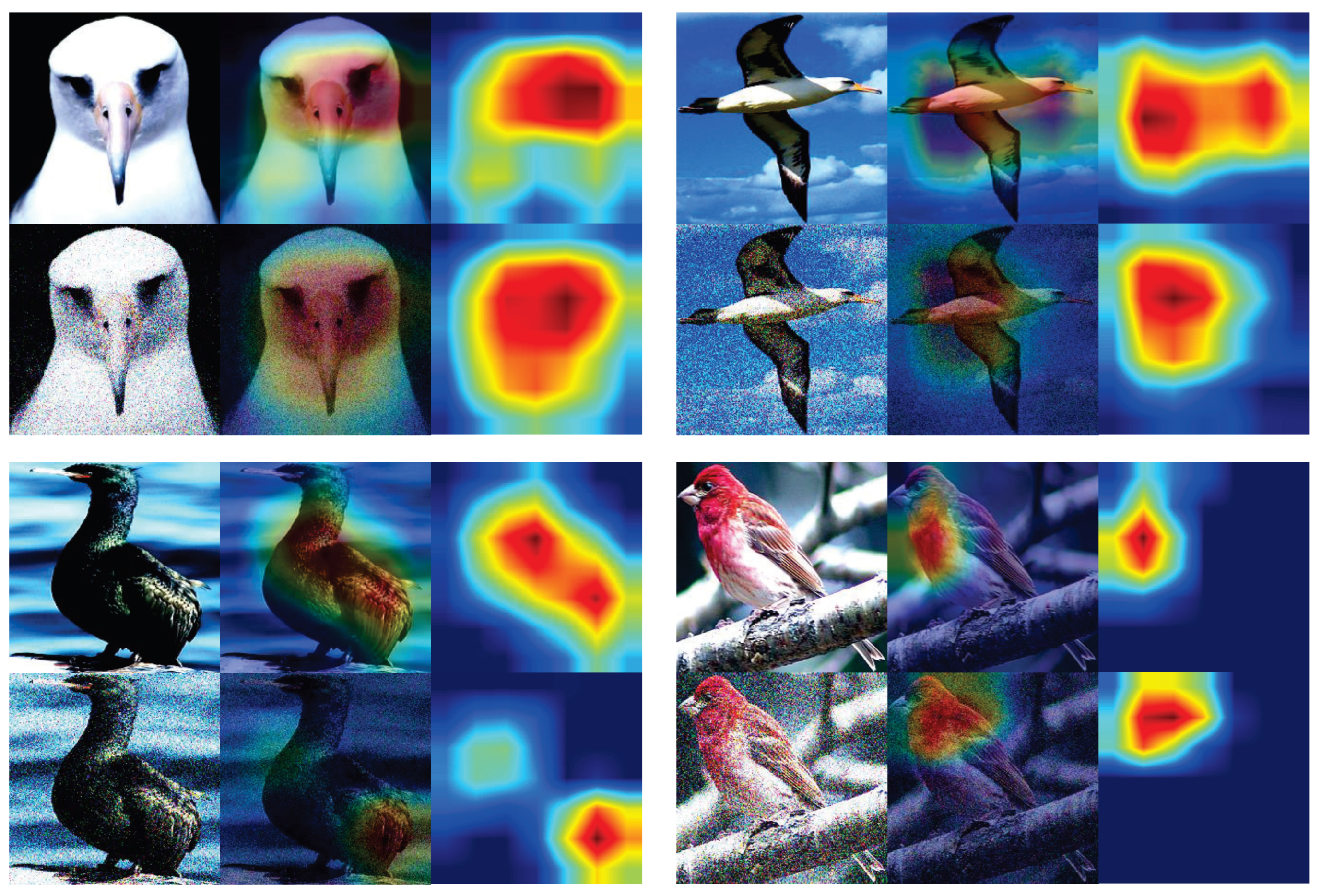
4.4. Interpretability Enhancement

We first conducted a qualitative study on the visual interpretability consistency of the proposed INNT. Keeping the network architecture and hyperparameters the same, we used the GradCAM algorithm to generate heatmaps for the last convolutional layer of each network. The results on the CUB-200-2011 and CIFAR-10 datasets are displayed in Figure 7.

As shown in Figure 7, in our approach, the heatmaps of clean images and noise images exhibit higher consistency compared to Noise Training (NT). This not only includes similar high-activation regions but also very close activation centers. The consistent visual results across different network architectures and datasets suggest that INNT is capable of successfully learning interpretable object features in the presence of noise interference, rather than blindly generalizing decision boundaries just to tolerate noise.

We also validated the effectiveness of INNT across different network architectures, as shown in Figure 8. Models trained with INNT demonstrate consistent interpretation regions on both clean and noisy images, even in cases with complex activation regions, such as the example of AlexNet with INNT on CIFAR-10.

In addition, to mitigate the potential influence of a single visualization explanation algorithm on the qualitative study, we also computed heatmaps using two other methods, GradCAM++ and ScoreCAM, as shown in Figure 9. Models trained with INNT exhibit consistent performance across all three visualization explanation algorithms, demonstrating clear consistency in the activation maps. This indicates that the interpretability brought about by INNT is independent of the specific visualization explanation algorithm used. It also enables us to proceed with quantitative research using the more concise form of GradCAM.

Finally, we conducted a quantitative study on the interpretability of INNT. By measuring the metrics mentioned in Section 4.3, namely AI, AD, and AEPE, we calculated these indicators using the GradCAM algorithm for each model under NT and INNT. The results are summarized in

Table 3. Comparative evaluation in terms of AI (higher is better), AD (lower is better), and AEPE (lower is better) scores. Bold represents the best.

Models		Gaussian Noise			Neighborhood Noise
		AD	AI	AEPE	AD	AI	AEPE
ResNet	ResNet	0.9216	0.0397	0.1158	0.8928	0.0405	0.1277
	ResNet NT	0.6283	0.1798	0.1277	0.5228	0.2008	0.0802
	ResNet INNT	0.4189	0.2354	0.0795	0.3067	0.2354	0.0547
VGG16	vgg16	0.7442	0.1591	0.1245	0.7191	0.0960	0.1037
	vgg16 NT	0.4730	0.2135	0.0871	0.3255	0.1798	0.0763
	vgg16 INNT	0.4097	0.2453	0.0738	0.3001	0.2211	0.0590
AlexNet	AlexNet	0.8002	0.1201	0.1576	0.7226	0.1463	0.1280
	AlexNet NT	0.5350	0.2781	0.1076	0.2699	0.3126	0.0724
	AlexNet INNT	0.4109	0.3013	0.1000	0.2078	0.3578	0.0395

. Our method achieved the highest faithfulness and localization ability in all cases, i.e., the highest Average Increase and the lowest Average Drop and Average Energy-based Pointing Error. The quantitative research results indicate, on one hand, that INNT enables the model to evaluate clean and noise images more faithfully, and on the other hand, that INNT constrains the model to rely more accurately on target information.

4.5. Predictive Performance

The Top-1 and Top-5 of all the models on the CUB-200-2011 test set are shown in

Table 4. Top-1, Top-5, and accuracy gap on the CUB-200-2011 test set for different models. Bold represents the best.

Models	Gaussian Noise						Neighborhood Noise
	Clean		Noise		Acc Gap		Clean		Noise		Acc Gap
	Top1%	Top5%	Top1%	Top5%	Top1%	Top5%	Top1%	Top5%	Top1%	Top5%	Top1%	Top5%
ResNet	81.50	95.71	31.78	57.42	49.72	38.29	81.50	95.71	46.72	71.65	34.78	24.06
NT	76.62	93.16	72.53	91.96	4.09	1.20	78.67	95.13	73.24	94.03	5.43	1.10
INNT	78.32	94.82	74.12	93.40	4.20	1.42	78.05	94.66	75.41	93.84	2.64	0.82
VGG16	73.79	93.65	15.21	33.88	58.58	59.77	74.32	93.13	33.46	59.65	40.86	33.48
NT	76.20	93.08	65.65	88.15	10.55	4.93	78.20	93.64	72.40	91.06	5.80	2.58
INNT	72.93	92.40	68.71	89.98	4.22	2.42	76.89	93.98	73.20	92.16	3.69	1.82
AlexNet	61.02	86.54	7.12	18.66	53.90	67.88	61.02	86.54	17.18	38.67	43.84	47.87
NT	49.58	79.66	39.95	69.44	9.63	10.22	52.75	79.54	47.43	74.36	5.43	5.18
INNT	57.87	83.73	54.94	80.88	2.93	2.85	58.34	85.38	54.23	81.64	4.11	3.74

. Additionally, we conducted the same experiment on the CIFAR-10 dataset, and the results are summarized in

Table 5. Top-1, Top-5, and accuracy gap on the CIFAR-10 test set for different models. Bold represents the best.

Models	Gaussian Noise						Neighborhood Noise
	Clean		Noise		Acc Gap		Clean		Noise		Acc Gap
	Top1%	Top5%	Top1%	Top5%	Top1%	Top5%	Top1%	Top5%	Top1%	Top5%	Top1%	Top5%
ResNet	96.76	99.94	18.63	81.69	78.13	18.25	96.76	99.94	52.78	94.52	43.98	5.42
NT	95.66	99.92	94.67	99.90	0.99	0.02	96.48	99.94	95.32	99.88	1.16	0.06
INNT	95.76	99.88	95.07	99.87	0.69	0.01	95.80	99.89	95.33	99.89	0.47	0.00
VGG16	92.93	99.87	10.01	50.43	82.92	49.44	92.93	99.87	11.67	60.26	81.26	39.61
NT	91.33	99.60	88.55	99.47	2.78	0.13	92.34	99.85	89.60	99.72	2.74	0.13
INNT	91.39	99.71	90.53	99.70	0.86	0.01	93.84	99.85	92.32	99.75	1.52	0.10
AlexNet	92.85	99.76	25.66	68.28	67.19	31.48	92.85	99.76	43.77	86.39	49.08	13.37
NT	90.83	99.73	89.76	99.63	1.07	0.10	92.25	99.79	90.52	99.66	1.73	0.13
INNT	90.64	99.74	90.17	99.69	0.47	0.05	91.43	99.75	90.88	99.72	0.55	0.03

. The results indicate that the accuracies of NT and INNT are at a comparable level, with no specific trend observed in the variation in INNT accuracy. However, when we calculate the difference in accuracy between clean and noisy data, we observe that INNT consistently reduces the accuracy gap between noisy images and original samples in most cases, aligning with our expectations.

Regarding the outlier in the Gaussian noise experiment on ResNet in CUB-200, although the accuracy gap under NT is smaller, the actual reduction rates of both accuracy gaps are only 2.6% and 15.5%. In contrast, under other superior INNT conditions, the reduction rates of the accuracy gap can reach 24.3% and 27.8% (in the neighborhood noise experiment of AlexNet, the reduction rate of the Top-1 accuracy gap is the smallest among all experiments). Considering the presence of random factors such as noise sampling in the tests, we believe that the Gaussian noise experiment on ResNet in CUB200 can be approximated to exhibit consistent performance in the accuracy gap between INNT and NT.

5. Conclusions

In this work, we proposed a novel interpretable noise training framework named Interpretable Neighborhood Noise Training (INNT). As a more reliable approach to noise training, we propose an end-to-end training procedure that involves iterative resampling of minute noise. Additionally, we propose a neighborhood noise sampling method as a complement to the noise function. By constraining the similarity of feature map activations, this method significantly enhances the neighborhood interpretation consistency of any CNN-based model. We have improved the evaluation metrics for saliency maps, conducting both qualitative and quantitative assessments of the interpretation enhancement while examining the performance of the original task. The research findings demonstrate that our training framework can reduce the model’s discrimination towards noisy samples while maintaining approximate accuracy, thereby aiding in the identification of more robust target features. We contend that any visually similar samples should be consistently decided upon by a robust model, and we aspire to discover more effective interpretable training methods in this manner. Thanks to INNT’s robust target feature learning capabilities and universal applicability to CNN models, INNT can potentially be applied to tasks such as image generation [38], super-resolution image reconstruction [39], visual re-ranking [40], and image style conversion [41]. Future work includes introducing adversarial perturbations, analyzing the interpretation consistency of adversarial defense, and endeavoring to unify the generalization approaches of natural perturbations and adversarial perturbations.

References

1. Szegedy, C.; Zaremba, W.; Sutskever, I.; Bruna, J.; Erhan, D.; Goodfellow, I.; Fergus, R. Intriguing properties of neural networks. In Proceedings of the 2nd International Conference on Learning Representations, ICLR 2014, Banff, AB, Canada, 14–16 April 2014. [Google Scholar]
2. Goodfellow, I.J.; Shlens, J.; Szegedy, C. Explaining and Harnessing Adversarial Examples. Stat 2015, 1050, 20. [Google Scholar]
3. Tsipras, D.; Santurkar, S.; Engstrom, L.; Turner, A.; Madry, A. Robustness May Be at Odds with Accuracy. In Proceedings of the International Conference on Learning Representations, New Orleans, LO, USA, 6–9 May 2019. [Google Scholar]
4. Rusak, E.; Schott, L.; Zimmermann, R.S.; Bitterwolf, J.; Bringmann, O.; Bethge, M.; Brendel, W. A simple way to make neural networks robust against diverse image corruptions. In Proceedings of the Computer Vision—ECCV 2020: 16th European Conference, Glasgow, UK, 23–28 August 2020; Proceedings, Part III 16. Springer: Berlin/Heidelberg, Germany, 2020; pp. 53–69. [Google Scholar]
5. Dodge, S.; Karam, L. Understanding how image quality affects deep neural networks. In Proceedings of the 2016 Eighth International Conference on Quality of Multimedia Experience (QoMEX), Lisbon, Portugal, 6–8 June 2016; pp. 1–6. [Google Scholar]
6. Geirhos, R.; Janssen, D.H.; Schütt, H.H.; Rauber, J.; Bethge, M.; Wichmann, F.A. Comparing deep neural networks against humans: Object recognition when the signal gets weaker. arXiv 2017, arXiv:1706.06969. [Google Scholar]
7. Hendrycks, D.; Dietterich, T. Benchmarking Neural Network Robustness to Common Corruptions and Perturbations. In Proceedings of the International Conference on Learning Representations, Vancouver, BC, Canada, 30 April–3 May 2018. [Google Scholar]
8. Cordts, M.; Omran, M.; Ramos, S.; Rehfeld, T.; Enzweiler, M.; Benenson, R.; Franke, U.; Roth, S.; Schiele, B. The Cityscapes Dataset for Semantic Urban Scene Understanding. In Proceedings of the IEEE Conference on Computer Vision and Pattern Recognition (CVPR), Las Vegas, NV, USA, 27–30 June 2016. [Google Scholar]
9. Mu, N.; Gilmer, J. Mnist-c: A robustness benchmark for computer vision. arXiv 2019, arXiv:1906.02337. [Google Scholar]
10. Moosavi-Dezfooli, S.M.; Fawzi, A.; Frossard, P. Deepfool: A simple and accurate method to fool deep neural networks. In Proceedings of the IEEE Conference on Computer Vision and Pattern Recognition, Las Vegas, NV, USA, 26 June–1 July 2016; pp. 2574–2582. [Google Scholar]
11. Rony, J.; Granger, E.; Pedersoli, M.; Ben Ayed, I. Augmented Lagrangian Adversarial Attacks. In Proceedings of the IEEE/CVF International Conference on Computer Vision (ICCV), Montreal, BC, Canada, 11–17 October 2021; pp. 7738–7747. [Google Scholar]
12. Duan, R.; Chen, Y.; Niu, D.; Yang, Y.; Qin, A.K.; He, Y. AdvDrop: Adversarial Attack to DNNs by Dropping Information. In Proceedings of the IEEE/CVF International Conference on Computer Vision (ICCV), Montreal, BC, Canada, 11–17 October 2021; pp. 7506–7515. [Google Scholar]
13. Michaelis, C.; Mitzkus, B.; Geirhos, R.; Rusak, E.; Bringmann, O.; Ecker, A.S.; Bethge, M.; Brendel, W. Benchmarking robustness in object detection: Autonomous driving when winter is coming. arXiv 2019, arXiv:1907.07484. [Google Scholar]
14. Mahajan, D.; Girshick, R.; Ramanathan, V.; He, K.; Paluri, M.; Li, Y.; Bharambe, A.; Van Der Maaten, L. Exploring the limits of weakly supervised pretraining. In Proceedings of the European Conference on Computer Vision (ECCV), Munich, Germany, 8–14 September 2018; pp. 181–196. [Google Scholar]
15. Laermann, J.; Samek, W.; Strodthoff, N. Achieving generalizable robustness of deep neural networks by stability training. In Pattern Recognition, Proceedings of the 41st DAGM German Conference, DAGM GCPR 2019, Dortmund, Germany, 10–13 September 2019; Springer: Berlin/Heidelberg, Germany, 2019; pp. 360–373. [Google Scholar]
16. Xie, Q.; Luong, M.T.; Hovy, E.; Le, Q.V. Self-training with noisy student improves imagenet classification. In Proceedings of the IEEE/CVF Conference on Computer Vision and Pattern Recognition, Seattle, WA, USA, 13–19 June 2020; pp. 10687–10698. [Google Scholar]
17. Zhang, R. Making convolutional networks shift-invariant again. In Proceedings of the International Conference on Machine Learning. PMLR, Long Beach, CA, USA, 9–15 June 2019; pp. 7324–7334. [Google Scholar]
18. Schneider, S.; Rusak, E.; Eck, L.; Bringmann, O.; Brendel, W.; Bethge, M. Improving robustness against common corruptions by covariate shift adaptation. Adv. Neural Inf. Process. Syst. 2020, 33, 11539–11551. [Google Scholar]
19. Pang, T.; Lin, M.; Yang, X.; Zhu, J.; Yan, S. Robustness and accuracy could be reconcilable by (proper) definition. In Proceedings of the International Conference on Machine Learning. PMLR, Baltimore, MI, USA, 17–23 July 2022; pp. 17258–17277. [Google Scholar]
20. Mikołajczyk, A.; Grochowski, M. Data augmentation for improving deep learning in image classification problem. In Proceedings of the 2018 International Interdisciplinary PhD Workshop (IIPhDW), Piscataway, NJ, USA, 9–12 May 2018; pp. 117–122. [Google Scholar]
21. Bishop, C.M. Training with noise is equivalent to Tikhonov regularization. Neural Comput. 1995, 7, 108–116. [Google Scholar] [CrossRef]
22. Gilmer, J.; Ford, N.; Carlini, N.; Cubuk, E. Adversarial Examples Are a Natural Consequence of Test Error in Noise. In Proceedings of the 36th International Conference on Machine Learning Research, Long Beach, CA, USA, 9–15 June 2019; Chaudhuri, K., Salakhutdinov, R., Eds.; IEEE: New York, NY, USA, 2019; Volume 97, pp. 2280–2289. [Google Scholar]
23. Vasiljevic, I.; Chakrabarti, A.; Shakhnarovich, G. Examining the impact of blur on recognition by convolutional networks. arXiv 2016, arXiv:1611.05760. [Google Scholar]
24. Zhang, Q.; Wu, Y.N.; Zhu, S.C. Interpretable convolutional neural networks. In Proceedings of the IEEE Conference on Computer Vision and Pattern Recognition, Salt Lake City, UT, USA, 18–23 June 2018; pp. 8827–8836. [Google Scholar]
25. Kuo, C.C.J. Understanding convolutional neural networks with a mathematical model. J. Vis. Commun. Image Represent. 2016, 41, 406–413. [Google Scholar] [CrossRef]
26. Wachter, S.; Mittelstadt, B.; Russell, C. Counterfactual explanations without opening the black box: Automated decisions and the GDPR. Harv. J. Law Technol. 2017, 31, 841. [Google Scholar] [CrossRef]
27. Zeiler, M.D.; Fergus, R. Visualizing and understanding convolutional networks. In Computer Vision—ECCV 2014, Proceedings of the 13th European Conference, Zurich, Switzerland, 6–12 September 2014; Part I 13; Springer: Berlin/Heidelberg, Germany, 2014; pp. 818–833. [Google Scholar]
28. Erhan, D.; Bengio, Y.; Courville, A.; Vincent, P. Visualizing higher-layer features of a deep network. Univ. Montr. 2009, 1341, 1. [Google Scholar]
29. Zhou, B.; Khosla, A.; Lapedriza, A.; Oliva, A.; Torralba, A. Learning deep features for discriminative localization. In Proceedings of the IEEE Conference on Computer Vision and Pattern Recognition, Las Vegas, NV, USA, 26 June–1 July 2016; pp. 2921–2929. [Google Scholar]
30. Selvaraju, R.R.; Cogswell, M.; Das, A.; Vedantam, R.; Parikh, D.; Batra, D. Grad-cam: Visual explanations from deep networks via gradient-based localization. In Proceedings of the IEEE International Conference on Computer Vision, Venice, Italy, 22–29 October 2017; pp. 618–626. [Google Scholar]
31. Chattopadhay, A.; Sarkar, A.; Howlader, P.; Balasubramanian, V.N. Grad-cam++: Generalized gradient-based visual explanations for deep convolutional networks. In Proceedings of the 2018 IEEE Winter Conference on Applications of Computer Vision (WACV), Lake Tahoe, NV, USA, 12–15 March 2018; pp. 839–847. [Google Scholar]
32. Wang, H.; Wang, Z.; Du, M.; Yang, F.; Zhang, Z.; Ding, S.; Mardziel, P.; Hu, X. Score-CAM: Score-weighted visual explanations for convolutional neural networks. In Proceedings of the IEEE/CVF Conference on Computer Vision and Pattern Recognition Workshops, Seattle, WA, USA, 14–19 June 2020; pp. 24–25. [Google Scholar]
33. Jiang, P.T.; Zhang, C.B.; Hou, Q.; Cheng, M.M.; Wei, Y. Layercam: Exploring hierarchical class activation maps for localization. IEEE Trans. Image Process. 2021, 30, 5875–5888. [Google Scholar] [CrossRef] [PubMed]
34. Bau, D.; Zhou, B.; Khosla, A.; Oliva, A.; Torralba, A. Network dissection: Quantifying interpretability of deep visual representations. In Proceedings of the IEEE Conference on Computer Vision and Pattern Recognition, Honolulu, HI, USA, 21–26 July 2017; pp. 6541–6549. [Google Scholar]
35. Cohen, J.; Rosenfeld, E.; Kolter, Z. Certified adversarial robustness via randomized smoothing. In Proceedings of the International Conference on Machine Learning—PMLR, Long Beach, CA, USA, 9–15 June 2019; pp. 1310–1320. [Google Scholar]
36. Wah, C.; Branson, S.; Welinder, P.; Perona, P.; Belongie, S. Caltech-UCSD Birds 200; Technical Report CNS-TR-2011-001; California Institute of Technology: Pasadena, CA, USA, 2011. [Google Scholar]
37. Krizhevsky, A.; Hinton, G. Learning Multiple Layers of Features from Tiny Images; University of Toronto: Toronto, ON, Canada, 2009. [Google Scholar]
38. Chen, X.; Duan, Y.; Houthooft, R.; Schulman, J.; Sutskever, I.; Abbeel, P. Infogan: Interpretable representation learning by information maximizing generative adversarial nets. Adv. Neural Inf. Process. Syst. 2016, 29, 2180–2188. [Google Scholar]
39. Dong, C.; Loy, C.C.; He, K.; Tang, X. Image super-resolution using deep convolutional networks. IEEE Trans. Pattern Anal. Mach. Intell. 2015, 38, 295–307. [Google Scholar] [CrossRef] [PubMed]
40. Bai, S.; Bai, X. Sparse contextual activation for efficient visual re-ranking. IEEE Trans. Image Process. 2016, 25, 1056–1069. [Google Scholar] [CrossRef] [PubMed]
41. Yu, Z.; Li, S.; Shen, Y.; Liu, C.H.; Wang, S. On the Difficulty of Unpaired Infrared-to-Visible Video Translation: Fine-Grained Content-Rich Patches Transfer. In Proceedings of the IEEE/CVF Conference on Computer Vision and Pattern Recognition, CVPR 2023, Vancouver, BC, Canada, 17–24 June 2023; pp. 1631–1640. [Google Scholar] [CrossRef]
Figure 1. INNT overview. In each mini-batch, given a clean image as input, we utilize the noise sample generation module to generate its corresponding noise sample. Then we forward propagate the clean and noise images through the convolutional layers of the CNN, obtaining feature maps for the different inputs. The L2 norm of the feature maps from both inputs is employed to compute the noise activation distance constraint regularization term. Simultaneously, forward propagation continues through linear layers to compute their respective classification losses. Finally, the combination of the noise activation distance constraint regularization term and the classification losses for both images is used as the overall loss function, which is then employed for backpropagation to update the CNN parameters.
Electronics 12 04751 g001
Figure 2. The noise training saliency maps trained by the GradCAM algorithm. The red area in the saliency map represents the greater impact of the corresponding area on classification. On the contrary, the closer to blue, the smaller the contribution to the final decision. Each set comprises the clean image and the noise image, displayed from (left) to (right) as follows: original image, fused heatmap, and original heatmap. The activated regions and the number of activated centers in the original and noise images are not entirely identical.
Electronics 12 04751 g002
Figure 3. Decision boundary generalization induced by noise training. The generalization of decision boundaries due to noise training may result in overlapping decision radii for different classes, leading to noisy samples in the overlapping region being classified based on criteria different from clean samples.
Electronics 12 04751 g003
Figure 4. The sampling process of neighborhood noise. It illustrates the generation process of noise samples with a neighborhood radius of μ N = 1.0 and noise samples with μ N = 2.0 . Neighborhood noise is added to the target image at the pixel level, and the magnitude of the noise is controlled by the neighborhood radius μ N , where a larger μ N leads to more noise points.
Electronics 12 04751 g004
Figure 5. CUB-200-2011 dataset.
Electronics 12 04751 g005
Figure 6. The impact of noise with different parameters on predictive performance, illustrated with VGG16. We annotated the key points mentioned above.
Electronics 12 04751 g006
Figure 7. The evaluation of visual interpretability consistency between clean images and noisy images, with results shown for (a) CUB-200-2011 and (b) CIFAR-10. Each distinct sample contains the original image of the sample along with its corresponding Gaussian noise version (the second row) and neighborhood noise version (the fourth row). The saliency maps for ResNet under different noise and training methods are displayed in each column. The results indicate that INNT performs similarly on both types of noise, effectively addressing the issue of regional inconsistency observed in NT.
Electronics 12 04751 g007
Figure 8. The visual interpretability consistency evaluation of AlexNet and VGG16 on different datasets; all training employs Gaussian noise.
Electronics 12 04751 g008
Figure 9. The influence of different visualization algorithms on our method and NT. Our method consistently demonstrates superior activation region consistency compared to NT across three algorithms.
Electronics 12 04751 g009