Objective Video Quality Assessment and Ground Truth Coordinates for Automatic License Plate Recognition ^†

Abstract

In the realm of modern video processing systems, traditional metrics such as the Peak Signal-to-Noise Ratio and Structural Similarity are often insufficient for evaluating videos intended for recognition tasks, like object or license plate recognition. Recognizing the need for specialized assessment in this domain, this study introduces a novel approach tailored to Automatic License Plate Recognition (ALPR). We developed a robust evaluation framework using a dataset with ground truth coordinates for ALPR. This dataset includes video frames captured under various conditions, including occlusions, to facilitate comprehensive model training, testing, and validation. Our methodology simulates quality degradation using a digital camera image acquisition model, representing how luminous flux is transformed into digital images. The model’s performance was evaluated using Video Quality Indicators within an OpenALPR library context. Our findings show that the model achieves a high F-measure score of 0.777, reflecting its effectiveness in assessing video quality for recognition tasks. The proposed model presents a promising avenue for accurate video quality assessment in ALPR tasks, outperforming traditional metrics in typical recognition application scenarios. This underscores the potential of the methodology for broader adoption in video quality analysis for recognition purposes.

1. Introduction

The evaluation of video quality varies depending on the application. Although the quality of entertainment videos focuses primarily on viewer satisfaction, the quality assessment of Target Recognition Videos (TRVs) emphasizes the utility of video for specific tasks, such as video surveillance, telemedicine, fire safety, and more [1,2]. In the domain of TRVs, current quality predictors, mostly developed based on subjective assessments, often fail to accurately reflect the needs of recognition tasks. These predictors do not adequately address unique challenges such as variable lighting conditions, motion blur, or occlusion, which are critical for tasks such as surveillance and Automatic License Plate Recognition. This disconnect between subjective quality measures and the actual utility of TRVs in practical applications highlights a significant gap in the current approach to video quality assessment in these contexts [2].

While traditional methods of quality assessment like Full Reference (FR) and No Reference (NR) metrics work well for standard videos, they do not consider the particular characteristics that are vital for the performance of Target Recognition Videos (TRVs). These methods often overlook factors such as target visibility under varying conditions, which are vital for accurate recognition. As a result, there is a noticeable gap in the literature, particularly regarding the objective evaluation of TRVs in both manual and automated recognition tasks.

In this paper, we aim to bridge this gap by introducing an objective evaluation methodology that is specifically designed for TRVs. Our approach focuses on creating a comprehensive dataset geared towards Automatic License Plate Recognition, encompassing various real-world challenges such as occlusion and low light. Using this dataset, we design, develop, and test a system that is capable of predicting the performance of machine vision algorithms based on the quality of incoming TRVs. Our primary goal is to demonstrate the feasibility of constructing accurate models that can anticipate the effectiveness of TRV processing pipelines in a broad range of scenarios.

The principal contributions of this work are

• The introduction of an objective evaluation methodology tailored to TRVs, filling a significant gap in the existing literature;
• The presentation of a comprehensive dataset for Automatic License Plate Recognition, simulating a spectrum of real-world conditions;
• The development and validation of a predictive system that employs Video Quality Indicators to gauge the machine vision performance in TRV tasks, which is beneficial to both academic research and industry applications;
• A comparative analysis of existing methodologies, asserting the advantages and broader applicability of the proposed approach;
• Selected elements of examination of the implications of existing legal regulations on the TRV quality, emphasizing the importance of this work in ensuring adherence to technical specifications while maintaining the functional efficacy.

Together, these contributions strive to advance the domain of video quality evaluation, especially in areas that require highly accurate target identification, such as systems for automatically recognizing vehicle license plates.

Our work differs significantly from existing efforts in several aspects. Although there are initiatives that address the TRV quality evaluation [3,4,5,6,7,8,9], they primarily focus on specialized domains such as public safety or health care and do not directly address the nuances involved in Automatic License Plate Recognition. Furthermore, while there are established benchmarks in video quality assessment, such as KoNViD-1k [10], LIVE-VQC [11], YouTube-UGC [12], and LSVQ [13], our work provides a more holistic approach, focusing on the creation of universal objective evaluation metrics for TRVs designed specifically for Automatic License Plate Recognition scenarios. This underscores the necessity of our custom dataset, which is meticulously curated to address unique challenges in this field. Legal regulations often dictate technical specifications in some TRV applications [1,2], further underscoring the need for objective quality assessment methods that can ensure compliance while maintaining effectiveness. The remainder of this paper is organized as follows. Section 2 details the experimental design; Section 2.1 and Section 2.2 describe corpus collection and the development of degradation models, respectively; Section 2.3 and Section 2.4 explain the experiments conducted; Section 3 reports our findings; and Section 4 concludes the paper.

2. Materials & Methods

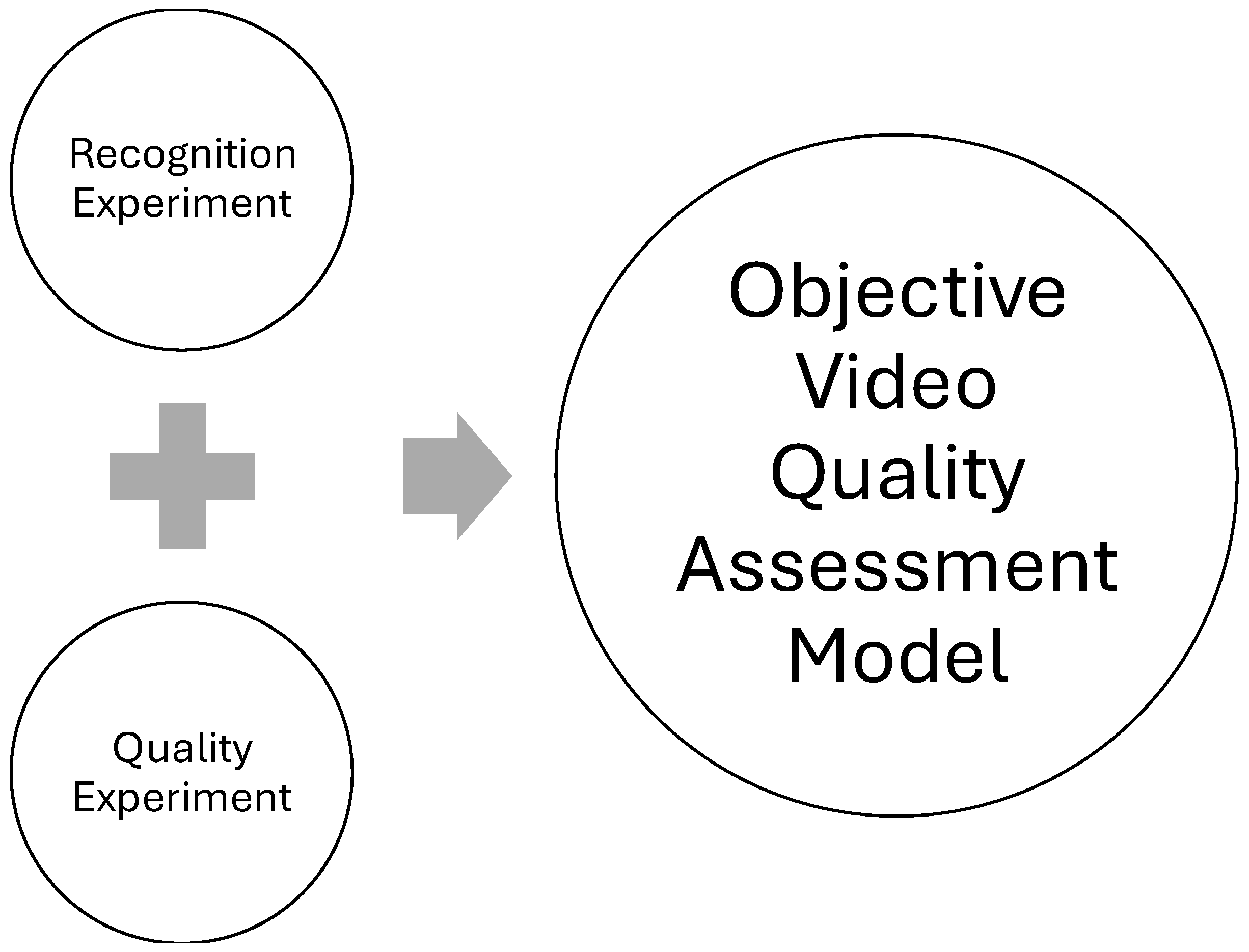
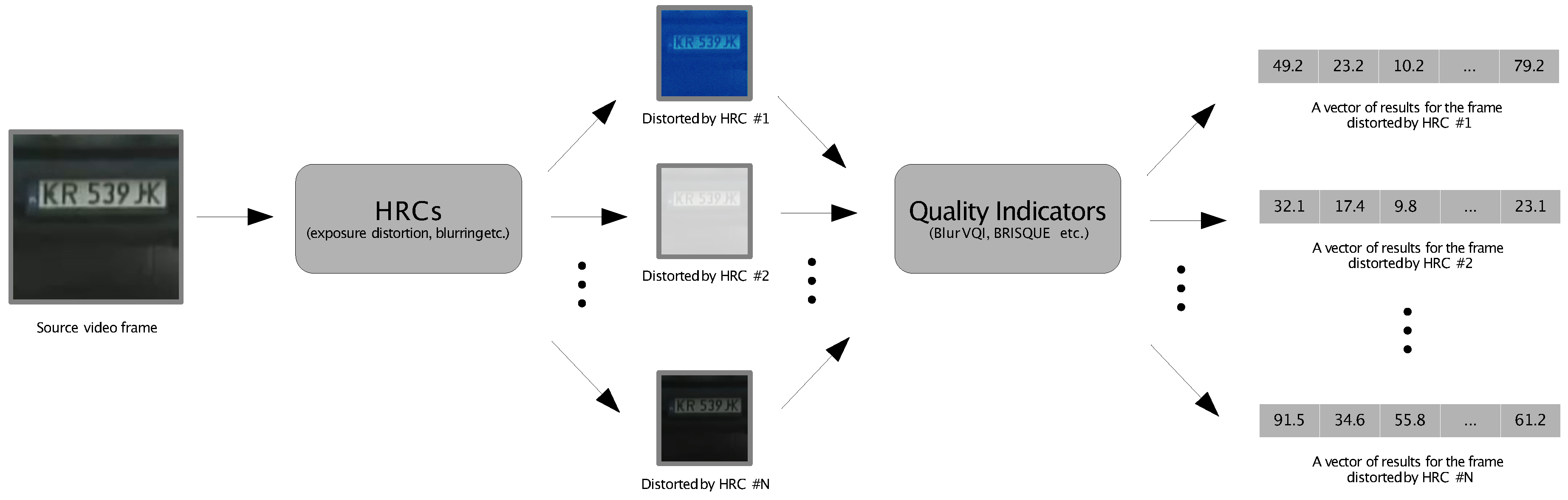
This section outlines the comprehensive methodology used in our study. Figure 1 illustrates the general methodology flow chart, which encapsulates the core components of our research approach. Our experimental framework integrates a foundational dataset (denoted the Source Reference Circuits, SRCs, Section 2.1) and a variety of visual impairments (termed Hypothetical Reference Circuits, HRCs, Section 2.2). Each HRC imposes a specific type of degradation on an SRC. The analysis of the output video sequences is conducted through a computer vision library for Automatic License Plate Recognition (ALPR, Section 2.3), combined with a Video Quality Indicator (VQI, Section 2.4).

2.1. Collection of Pre-Existing Source Reference Circuits (SRCs)

This subsection delineates the technical attributes of the chosen SRCs and the specially assembled dataset used in this investigation. The corpus consisting of pre-existing original SRC video sequences was utilized.

The SRC repository encompasses a variety of video frames chosen according to a criterion aimed at compiling a comprehensive database encompassing a diverse array of characteristics. The details of the dataset are explained in the following section.

Within the scope of our experimental framework, a subset of the entire SRC collection was used. The initial step in curating this subset involved determining its magnitude. To this end, preliminary experimental runs, potential subsequent training iterations, and a validation experiment for the model were envisaged. The validation set is substantial, comprising roughly a quarter of the volume of a single training session, while the initial and any potential second training phases are composed of an equivalent number of samples.

An additional premise adopted for the experimental design, grounded in pragmatic considerations, stipulates that the duration of an experimental iteration shall not exceed one week. This temporal constraint influences the scale of the training sets, considering that the size of the test sets is a quarter of that of the training sets.

At this juncture, it is imperative to recognize that the computation time for a single frame exerts a significant impact on the volume of frames incorporated into each experiment. This time frame encompasses the aggregate duration of image processing for both the quality experiment (Section 2.4) and the recognition experiment (Section 2.3). With an understanding of the mean time taken to conduct the quality experiment on an individual frame and the mean time for the recognition experiment on the same, we are able to approximate the quantity of frames that can be processed weekly or the total number of frames that can be accommodated in a single experimental cycle.

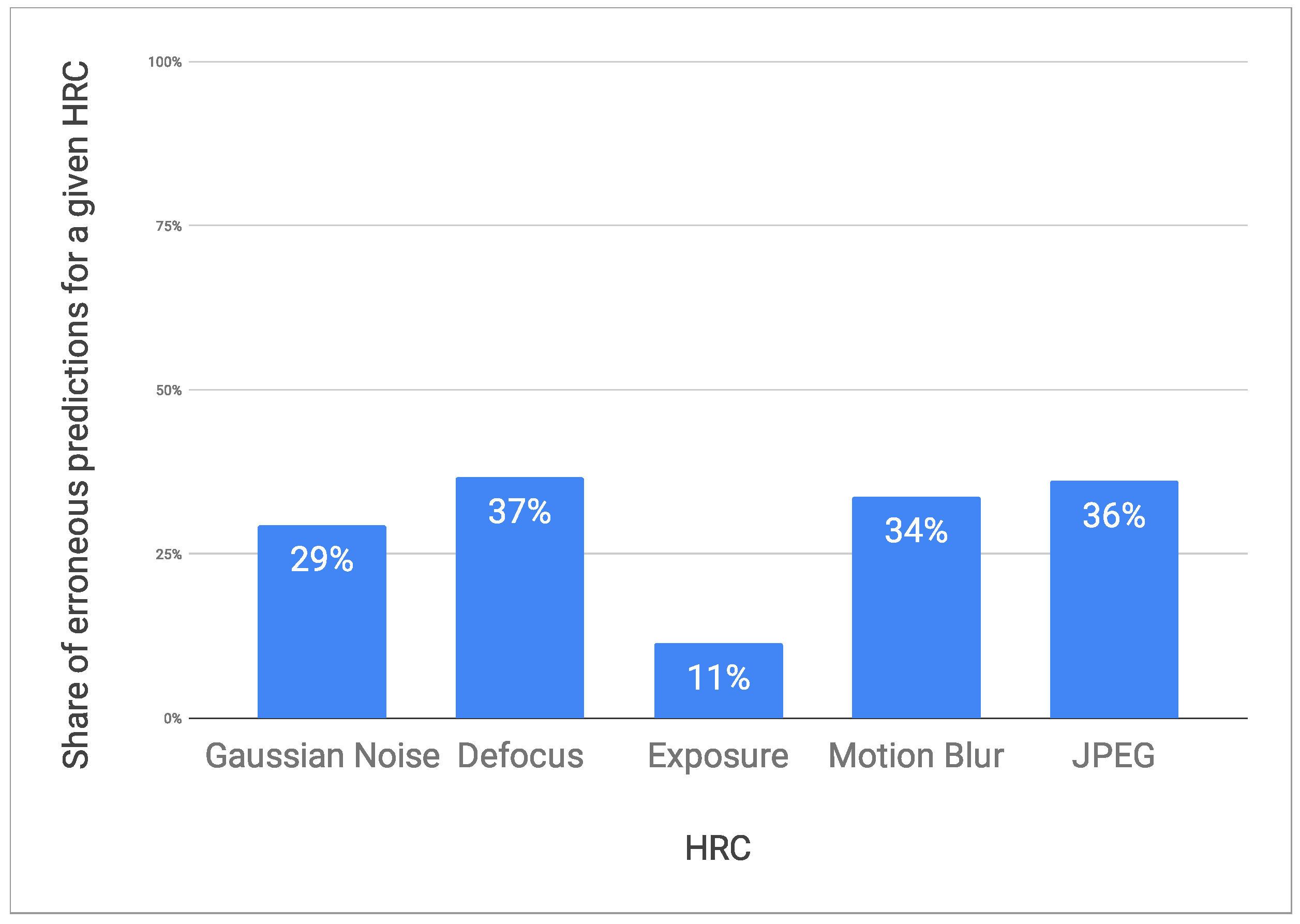
Furthermore, it is essential to clarify that the figure yielded by the aforementioned procedure pertains to the count of feasible Processed Video Sequence (PVS) frames, as opposed to the count of utilizable SRC frames. To ascertain the tally of employable SRC frames, we take the total number of viable PVS frames and divide it by the quantity of the stipulated HRCs. The aggregate of the HRCs, including the original SRC, is 65.

Progressing to particular details, it has been ascertained that the average duration for processing a singular image in the quality experiment is within the magnitude of hundreds of seconds. In contrast, the average time taken to process an image in the recognition experiment is less than a second, which renders it comparatively negligible.

In light of the previously stated considerations, within a weekly time frame, it is feasible to process PVS images derived from 120 distinct SRC images. This allocation permits the arrangement of 80 SRC images for the initial training experiment, with an additional set of 20 SRC images (a quarter of the training set) for the testing phase and a further 20 SRC images (another quarter) for validation purposes. Each SRC image features a singular discernible entity (a vehicle’s license plate), culminating in a total of 120 individual entities.

As delineated earlier, a validation set of equivalent size to the test set has been assembled but is currently not processed.

Subsequent segments of this subsection elaborate on the complete collection (Section 2.1.1) and the specific selection utilized for the experiment (Section 2.1.2).

2.1.1. The Automatic License Plate Recognition Data Collection

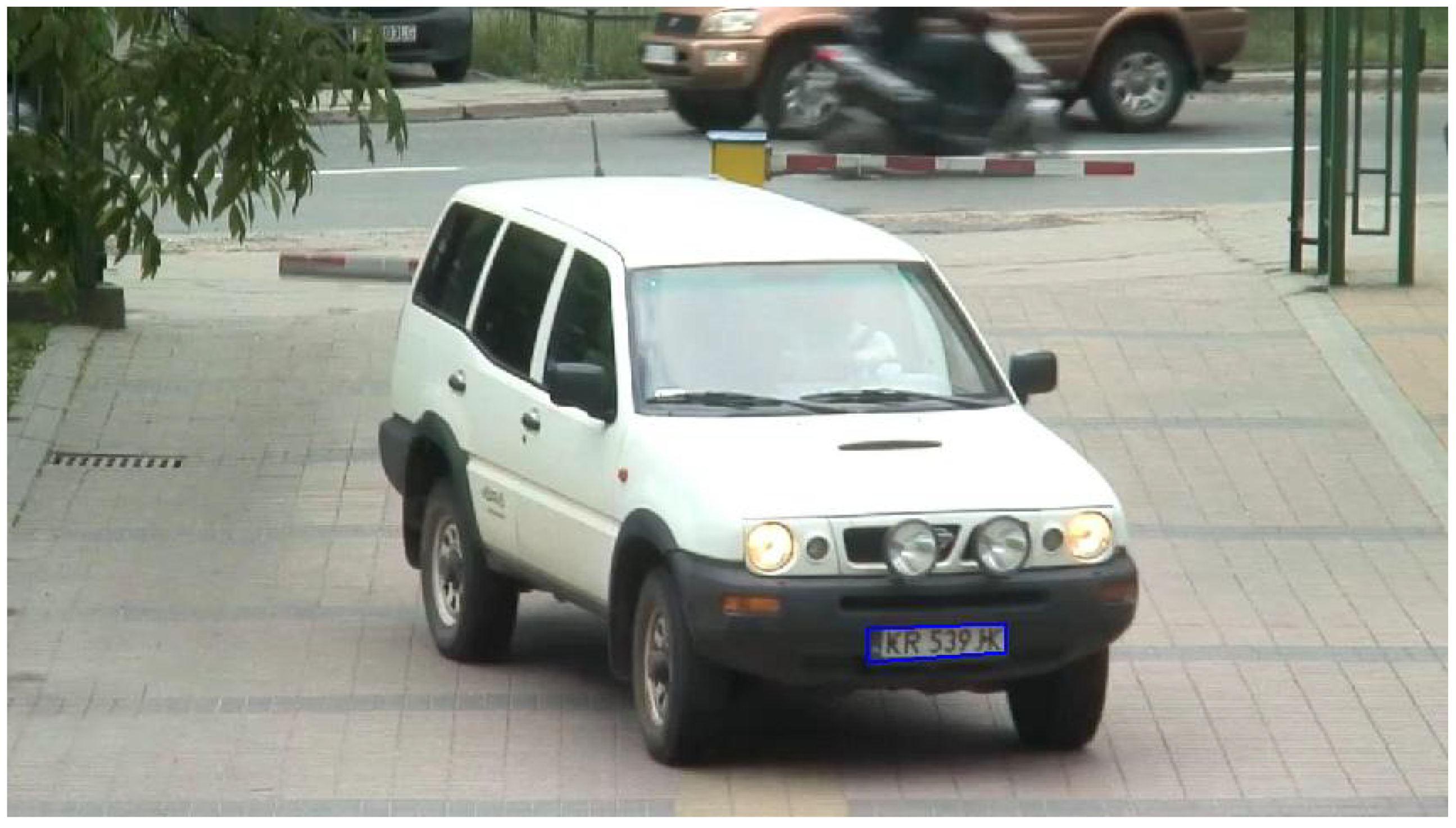
The ALPR dataset examined was curated from CCTV footage. The video sequences of the source reference circuit (SRC) were recorded at the AGH University of Krakow, Lesser Poland, focusing on high traffic parking areas during peak hours [2]. The compiled dataset encompasses approximately 15,500 frames in total.

Ground Truth Annotation

Ground truth coordinates were prepared to facilitate the assessment of Automatic License Plate Recognition. For each video in the dataset, a corresponding text file containing ground truth information was created. These annotations were compiled in July 2019. The text file adheres to the following naming convention:

  video_name_anno.txt

Each of these files lists the coordinates specifying the location of the license plate in individual frames.

Coordinate Formatting

Within each ground truth file, the coordinates are formatted as follows:

  image_number.jpg,X1,Y1,X2,Y2,X3,Y3,X4,Y4

An example line could look like the following:

  1.jpg 511 137 582 136 582 154 512 154

Coordinate Significance

The coordinates $(X1,Y1),(X2,Y2),(X3,Y3),(X4,Y4)$ designate the following points on the license plate:

• $(X1,Y1)$: Top-left corner of the license plate;
• $(X2,Y2)$: Top-right corner of the license plate;
• $(X3,Y3)$: Bottom-right corner of the license plate;
• $(X4,Y4)$: Bottom-left corner of the license plate.

Special Cases

In cases where the license plate is fully occluded, all coordinates are annotated as zero. For example,

  50.jpg 0 0 0 0 0 0 0 0

For partially occluded license plates, only the visible portions are annotated in the ground truth file.

Data Availability

The entire dataset can be accessed in the “Supplementary Materials” section. A representative SRC frame is illustrated in Figure 2.

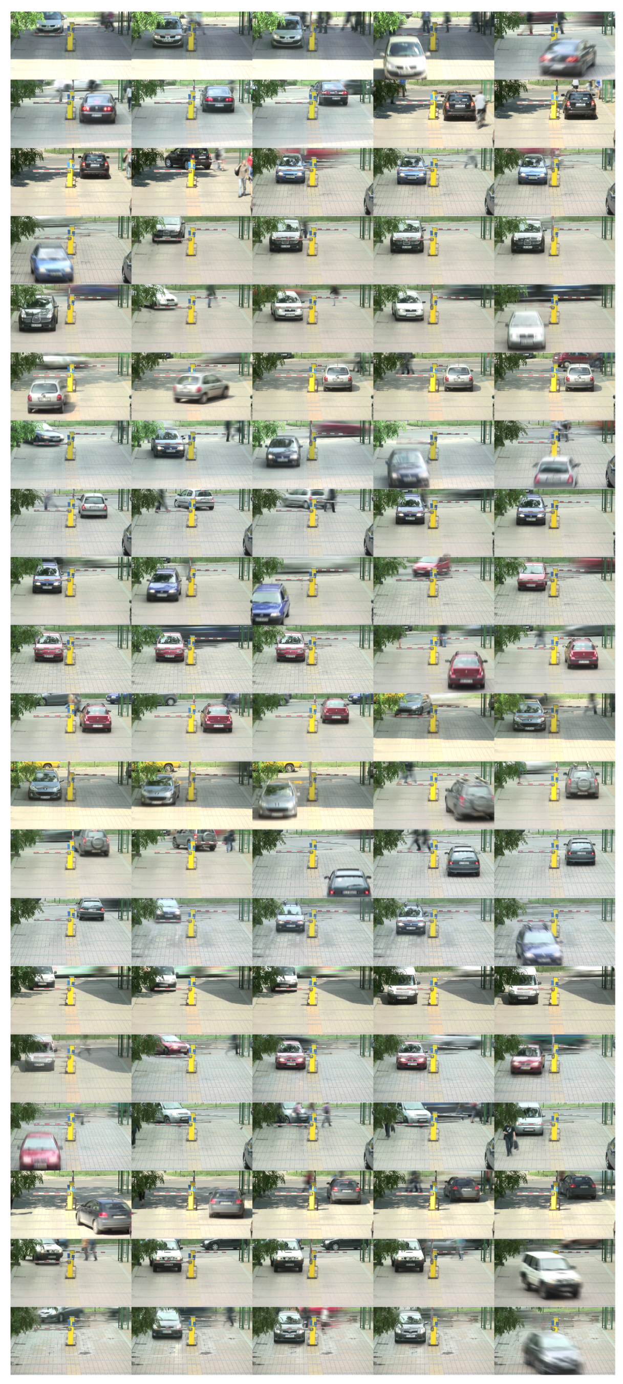
2.1.2. The ALPR Subset

A subset is derived from the full assembly, allocating 120 images in a training, testing, and validation array in ratios of 80, 20, and 20, respectively. A compilation of the SRC images chosen for ALPR is depicted in Figure 3.

Please refer to the Appendix A for the complete list.

2.2. Making Hypothetical Reference Circuits (HRC)

This section addresses the various degradation scenarios, termed Hypothetical Reference Circuits (HRCs). The proposed array of HRCs encompasses a variety of impairments throughout the digital image acquisition process. The choice of HRCs is pivotal as it influences the applicability of the quality assessment methodology suggested here.

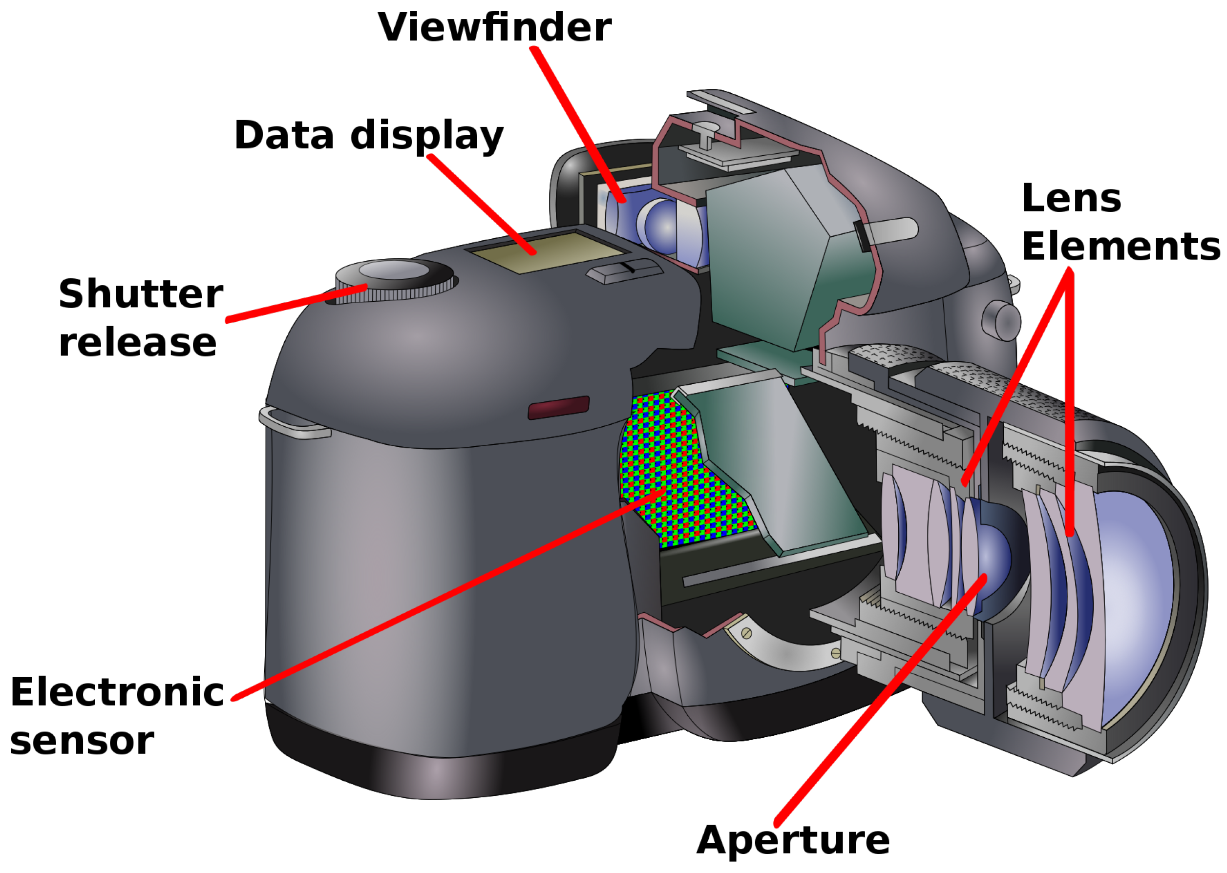
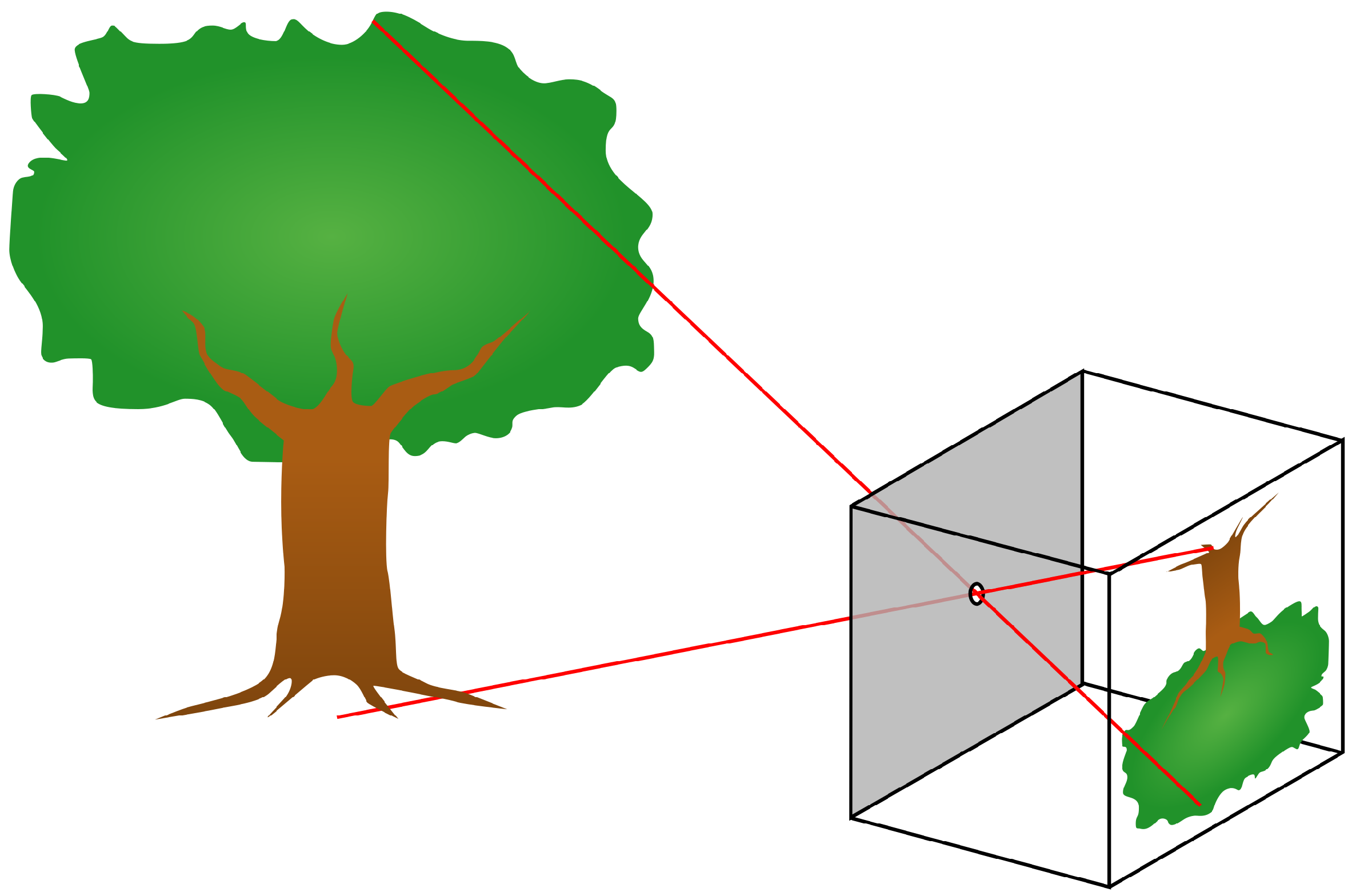
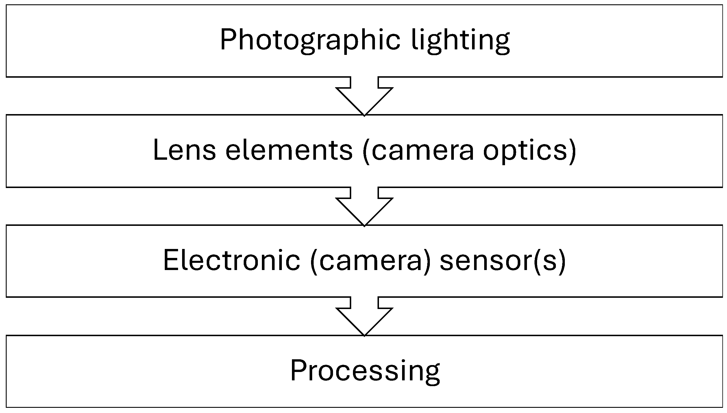
Currently, HRC selection utilizes two distinct types of camera model: a model of a digital single-lens reflex camera and a basic pinhole camera model. The latter is especially relevant to ALPR applications, as the detailed features of more elaborate camera models do not necessarily enhance the recognition task. The single lens reflex digital camera model is shown in Figure 4, while the pinhole camera model schematic is shown in Figure 5.

The operation of a digital camera is characterized by the manner in which light reflection from a subject is transformed into a digital image. Insufficient exposure to ambient light can attenuate the light before it reaches the lens system. Should the lens elements be misaligned, a blurred effect, known as defocus aberration, may ensue. Subsequently, the light interacts with an electronic sensor, the resolution of which is finite, potentially introducing Gaussian noise during analogue-to-digital conversion and subsequent signal amplification. Moreover, a prolonged exposure time can result in motion blur, while compression algorithms like JPEG may introduce artifacts in the final rendering of the digital image.

For the pinhole camera model, image formation is simplified; it assumes a single point where light rays pass through to form an image on an imaging surface. This model eliminates lens-induced aberrations, such as defocus and distortions. The simplicity of the pinhole camera model allows us to isolate other variables, such as exposure, motion blur, and sensor noise, in our quality assessment framework. The versatility of the pinhole camera model lies in its simplicity, which proves to be highly suitable for ALPR scenarios where diverse environmental factors, including fluctuating light conditions and varying distances from the camera to the license plate, can impact the quality of the captured image.

With this dual-model approach, we aim to offer a more comprehensive understanding of how different camera models can affect the quality and utility of TRVs in ALPR systems.

By incorporating the pinhole camera model into our HRC set, we aim to provide a more tailored approach to the evaluation of the video quality in ALPR applications. This modification aligns our work more closely with the practical needs of the ALPR community, which often employs simpler camera models because of their versatility and effectiveness across a wide range of conditions.

The distortion model is shown in Figure 6.

We selected the following HRCs:

• Photographic lighting HRC:

  1.

  Image under/overexposure

• Camera optics lens elements HRC:

  2.

  Defocus (blur)

• Electronic (camera) sensor(s) HRC:

  3.

  Gaussian noise

  4.

  Motion blur

• Processing HRC:

  5.

  JPEG compression

2.2.1. Overview

The selection was made to utilize HRCs by incorporating tools from the resources [14,15], namely FFmpeg and ImageMagick, which offer a comprehensive suite of relevant filters. These tools facilitate the generation of the various distortions required; FFmpeg is utilized for the application of Gaussian noise and the adjustment of exposure levels, while ImageMagick is deployed for JPEG compression, motion blur simulation, and defocus effect creation.

Under the most demanding conditions, which involve enabling all available filters, the processing capability of the tool reaches a rate of 439 frames per minute. This performance benchmark was established through tests conducted on a conventional laptop equipped with an Intel i5 3317U processor and 16 GB of RAM.

Table 1. Boundaries for specified Hypothetical Reference Circuits (HRCs)—representing different distortions cataloged in a row-wise manner (based on: [2]).

HRC	Unit	Min	Max
Under-Exposure	FFmpeg filter parameter	0	−0.6
Over-Exposure	FFmpeg filter parameter	0	0.6
Defocus (Blur)	ImageMagick filter parameter	0	6
Gaussian Noise	FFmpeg filter parameter	0	48
Motion Blur	ImageMagick filter parameter	0	18
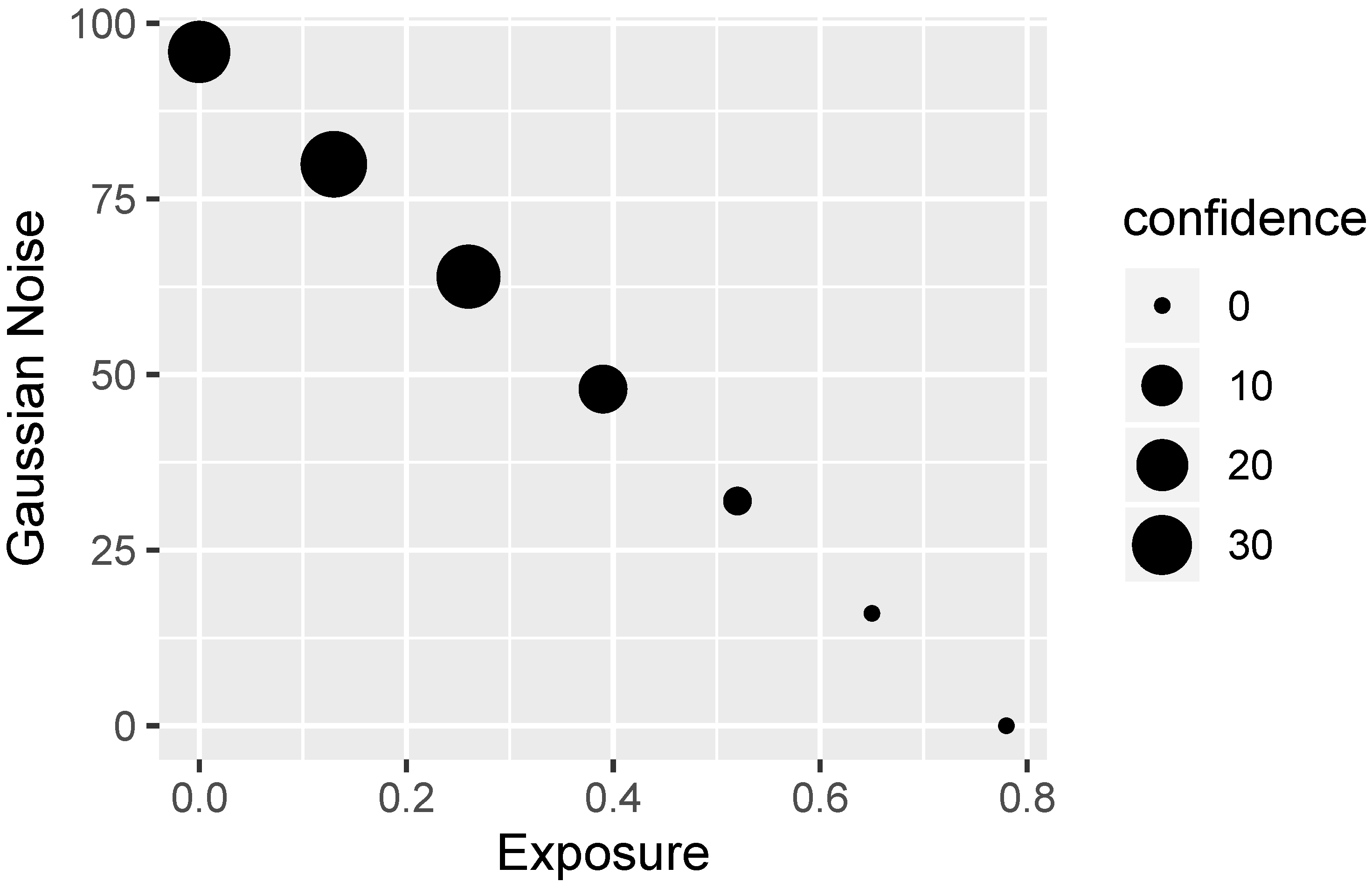
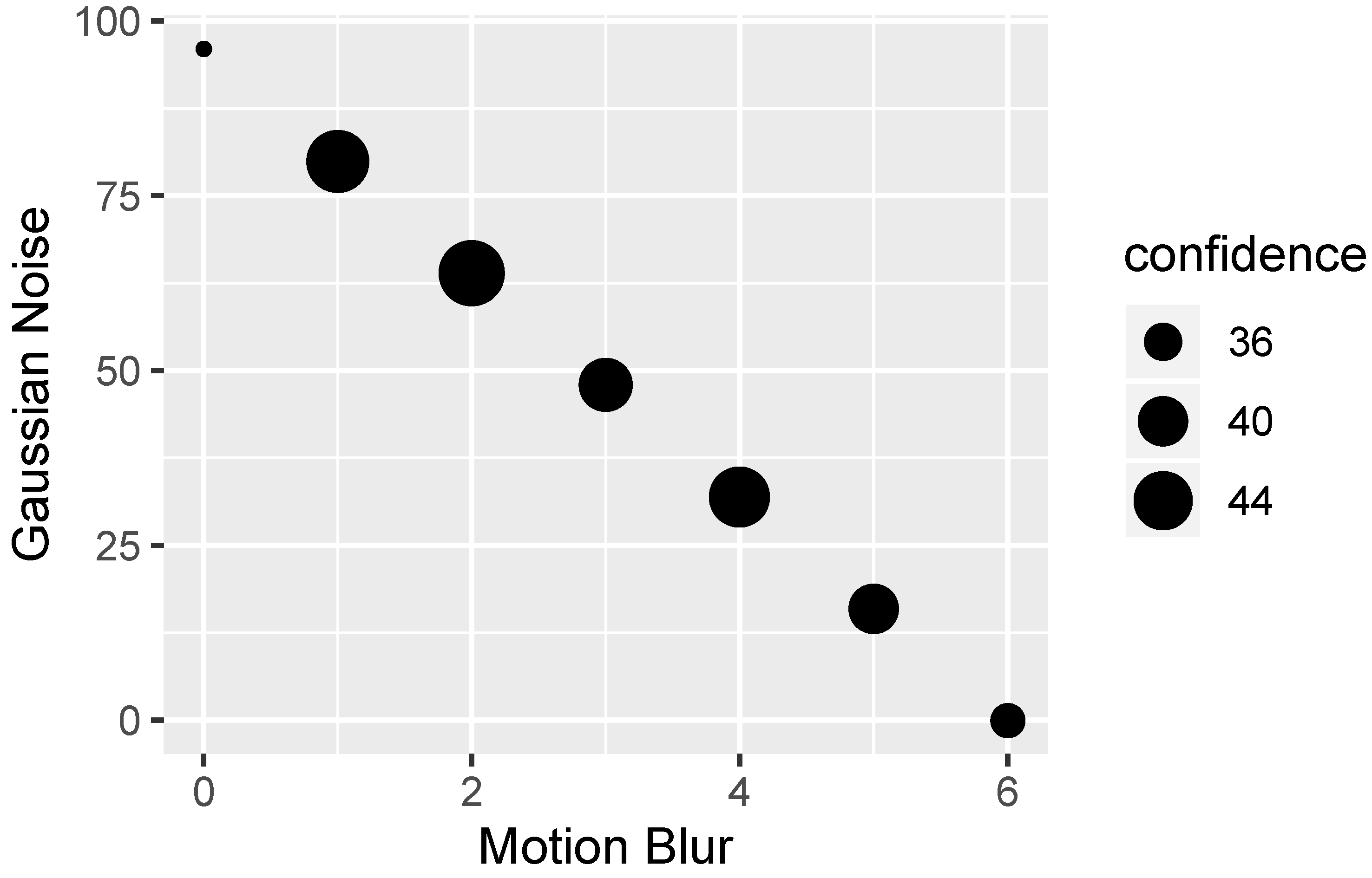
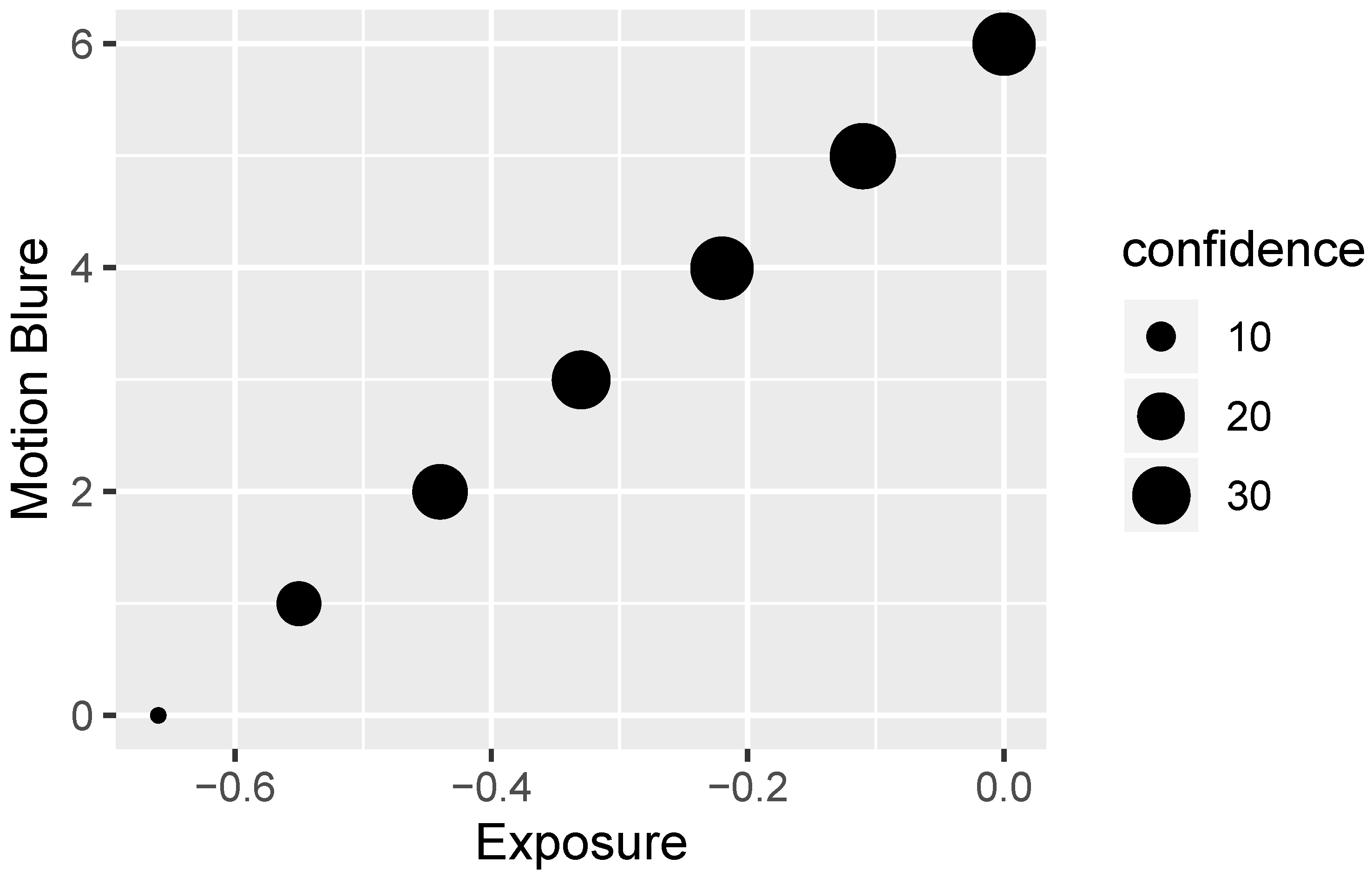
JPEG	ImageMagick filter parameter	0	100

presents the established thresholds for various types of distortion, which are itemized in the rows of the table. These thresholds are typically derived to pinpoint the HRC value at which recognition ceases to occur; this identification represents the next-to-last stage, with an additional margin incorporated for precautionary reasons. The sequence of determination is direct and methodical.

Table 2. Types of Distortion Arising from Hypothetical Reference Circuits, HRCs (reference: [2]).

HRC	#HRC
Over/Under-Exposure (Photography)	12
Defocus (Blur)	6
Gaussian Noise	6
Motion Blur	6
JPEG	19
Motion Blur + Gaussian Noise	5
Over-Exposure + Gaussian Noise	5
Under-Exposure + Motion Blur	5
#PVS	6720

outlines the specific distortions and provides an approximation of the number of intensity levels for each type of distortion. It is noted that most distortions are categorized into six intensity levels. Exceptions include JPEG compression and exposure alterations, which require the number of levels to be doubled to account for their bidirectional impacts. Moreover, when distortions are combined (as shown in the last three rows, each corresponding to a distinct subsection), only five levels are delineated, because the most severe levels are already captured in the creation of individual distortions (referenced in the preceding subsections of the table).

The order of distortion application is pivotal when employing multiple distortions:

• For the combination of motion blur and Gaussian noise, motion blur is applied initially;
• In the case of over-exposure combined with Gaussian noise, over-exposure precedes;
• For the under-exposure and motion blur combination, motion blur takes precedence due to technical constraints related to potential interpolation issues, despite under-exposure ideally being first.

Additionally, it is essential to include the scenario of “without distortion” (pristine SRC) within our distortion range. In total, this results in 64 HRC options (plus one unaltered SRC).

With the SRC selection finalized and the HRCs established, we can proceed to the actual video processing. This leads to the generation of a collection of processed video sequences, or PVSs, which are SRC frames affected by the HRC scenarios. The PVS corpus represents the anticipated result for this process.

The following is a detailed explanation of distortions and their applications. Our detailed description of the algorithms and configurations aims to add rigor and reproducibility to our methodology.

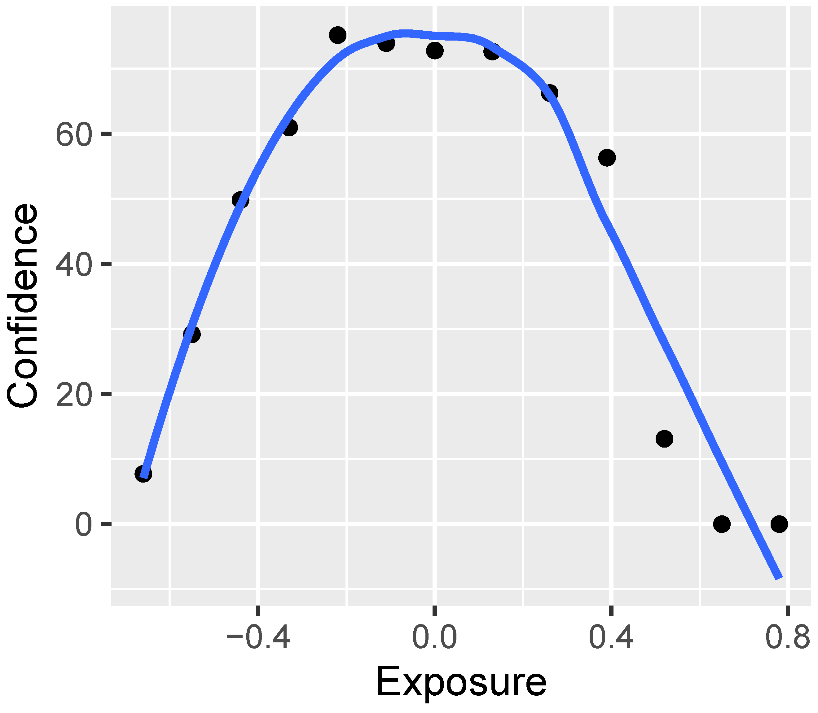
2.2.2. Exposure (Photography)

In the realm of photography, the term “exposure” delineates the quantum of light that reaches light-responsive substrates such as photographic film or digital sensors, playing an indispensable role in image capture. The exposure quotient is a composite function of the shutter velocity, the lens aperture scale, and the ISO sensitivity. Typically quantified in segments of seconds, exposure governs the duration that the aperture stays agape. An overabundance of light leads to overexposure, whereas a paucity thereof results in under-exposure [16].

In creating our HRC set, we utilized the FFmpeg library’s “eq” (equalizer) filter to adjust attributes such as exposure. The “eq” filter operates through pixel-level transformations that alter the brightness and contrast levels. It is mathematically defined as $P^{\prime }=(P-128)\times \mathrm{contrast}+128+\mathrm{brightness}$, where contrast and brightness are user-defined parameters.

The “eq” filter also supports adjustments to the saturation and gamma levels. Standard image processing techniques are generally applied. Saturation is adjusted using linear transformations in the color space, whereas gamma adjustments are made through a power-law function applied to intensity values.

For a complete list of permitted parameters and further details, consult the official FFmpeg documentation https://ffmpeg.org/ffmpeg-filters.html#eq (accessed on 14 November 2023).

Excess exposure makes vehicle registration plates appear white and unreadable, while insufficient exposure leads to dark patches within the image. Details in over-exposed or under-exposed areas are irrecoverable.

Through intentional over-exposure and under-exposure, the FFmpeg filter allows for a wide range of exposure adjustments. This facilitates the creation of HRCs to evaluate the performance of ALPR systems. Extreme exposure settings make the automobile registration plate unrecognizable to the human eye, ensuring that the HRC spans the full visible range.

2.2.3. Defocus

Defocus is a form of distortion that occurs when an image is not properly focused. This aberration affects various devices equipped with lenses, such as cameras, telescopes, or microscopes. Defocus diminishes image contrast and object sharpness, making well-defined, high-contrast edges appear blurry and eventually unidentifiable. On the contrary, excessive sharpening results in a noticeable grainy effect [17].

In our research, we used ImageMagick’s “blur” algorithm to introduce image distortions. The blur algorithm generally employs a Gaussian blur, characterized by a Gaussian distribution. It involves convolution with a Gaussian kernel, specified by two parameters: radius and standard deviation ($\sigma$). The Gaussian function is mathematically represented as $G(x,y)=\frac{1}{2\pi {\sigma }^2}{e}^{-\frac{x^2+y^2}{2{\sigma }^2}}$.

ImageMagick offers fine-tuning through various command-line options. For example, the “-channel” option applies blur to specific color channels, while “-motion-blur” introduces directional blur to simulate motion. Motion blur in ImageMagick uses a linear combination of pixels along a trajectory to mimic object movement.

For a complete list of available options and further details, consult the official ImageMagick documentation http://www.imagemagick.org/Usage/blur/#blur_args (accessed on 14 November 2023).

In this context, the sigma value serves as an estimate for pixel “dispersion” or blurring. According to the documentation, it is advisable to keep the radius parameter as small as possible.

ImageMagick enables accurate defocus degradation, allowing for precise adjustments. Even a slight change in the sigma parameter can make the vehicle registration plate unrecognizable. Consequently, in the generation of PVSs, it is imperative to administer the distortion at a level that precludes precipitous deterioration of the original material.

2.2.4. Gaussian Noise

Gaussian noise, recognized as statistical noise, exhibits a probability density function that conforms to a Gaussian distribution. Noise levels themselves follow a Gaussian distribution [18].

Cameras typically include an automated denoising algorithm. Our aim is not arbitrary noise introduction but rather realistic noise simulation. We add noise using FFmpeg’s “noise” filter and subsequently apply denoising.

For denoising, we employ FFmpeg’s “bm3d” filter, which uses the Block Matching and 3D Filtering (BM3D) algorithm. This technique uses the high level of redundancy in natural video to remove noise while preserving detail. The algorithm involves a two-step process: block matching and collaborative filtering. In our setup, the denoising strength ($\sigma$) is set to be equal to the added noise level, but it can be fine-tuned.

A higher noise value leads to significant visual distortions, complicating license plate recognition.

For more details, consult the FFmpeg documentation https://ffmpeg.org/ffmpeg-filters.html#bm3d (accessed on 14 November 2023).

2.2.5. Motion Blur

Motion blur appears as a motion streak and is only visible in sequences that feature moving objects. It occurs when the object being recorded changes position during shooting. The appearance of blurred motion can be attributed to a combination of the fast movement of objects and prolonged exposure [19].

Although FFmpeg does not provide a standalone motion blur filter, it offers filters such as “minterpolate” and “tblend” that can be configured to simulate motion blur. The “minterpolate” filter is based on motion estimation and frame interpolation algorithms, and “tblend” uses frame blending techniques. Although the specifics may vary depending on the filter configuration, these are general principles.

To simulate motion blur, we used ImageMagick’s radial blur function. This function is designed to simulate motion by convolving the image along a specific angle defined by the user, creating the appearance of a radial motion.

The function takes an angle parameter, which enables us to simulate different rotational speeds. A lower angle simulates slower rotation, while a higher angle indicates faster spin.

Among the various degradations, motion blur is often considered the most challenging. ImageMagick filters are our recommended solution to achieve optimal results when simulating motion blur degradation. For further information, see ImageMagick documentation at http://www.imagemagick.org/Usage/blur/#radial-blur (accessed on 14 November 2023).

2.2.6. JPEG

The JPEG standard is commonly used for image compression and is a popular digital format. It plays a pivotal role in the creation of billions of JPEG images each day, especially in digital photography [20].

We employ ImageMagick to compress the images to JPEG format, specifying the compression quality parameter using values ranging from 1 to 100: the lower the value, the higher the compression, and vice versa.

Lossy JPEG compression can cause recognizable artifacts, such as pixelation and a loss of fine details. In the case of license plates, higher compression ratios may render characters indistinct, complicating ALPR.

To optimize our methodology, we use the quality parameter to strike a balance between size and quality. The goal is to ensure that the compressed image retains enough quality to be useful for the evaluation of the ALPR system.

For details on ImageMagick’s JPEG compression options, consult the official documentation http://www.imagemagick.org/Usage/formats/#jpg (accessed on 14 November 2023).

2.3. Recognition Experiment

The organization of the recognition experiment is detailed in this subsection. An extensive overview is presented in the initial subsection (Section 2.3.1), followed by a more detailed description of the ALPR system in the next subsection (Section 2.3.2). The final subsection (Section 2.3.3) delves into the discussion of the execution time of ALPR.

2.3.1. Overview of the Recognition Experiment

Every PVS consists of a solitary frame, which is subsequently processed by an Automatic License Plate Recognition (ALPR) system. The flow chart in  Figure 7 illustrates the standard processing pipeline used in the recognition experiment.

2.3.2. ALPR System

The ALPR functionality is ensured by the OpenALPR library, which is implemented in C++. This library is designed to analyze images and videos for the detection and recognition of license plates. The algorithm employed by the library is capable of processing various types of image and videos. In the case of videos, the video file is divided into individual frames, and each frame is subjected to license plate detection and recognition. The library then returns ten potential license plates along with their corresponding confidence scores. Furthermore, an alternative exists to store the results in a JSON file that includes the coordinates of the identified license plate. Additionally, in light of the global diversity in license plate designs, OpenALPR offers a country code feature that enables the limitation of plate comparisons to a particular area, such as the EU or the US. This feature enhances both the confidence and efficiency of the recognition process. The Listing 1 illustrates an example of the output generated by OpenALPR for the recognition of license plates.

Listing 1. Example of the number plate recognition output.

The OpenALPR library is available on GitHub at https://github.com/openalpr/openalpr (accessed on 14 November 2023). It is dependent on two additional libraries: Tesseract and OpenCV. Tesseract, an optical character recognition engine, specializes in identifying and extracting text from images. On the other hand, OpenCV is utilized for image processing tasks within the library.

Figure 8, Figure 9, Figure 10, Figure 11, Figure 12, Figure 13, Figure 14 and Figure 15 display the impacts of various distortions on the confidence parameter of the ALPR system for the specified values.

2.3.3. ALPR Execution Time

To determine the number of SRCs that can be tested, it is essential to determine the duration required for all ALPR processes to compute, as mentioned previously. The computer vision algorithm employed for ALPR typically takes approximately 0.21 s to process a single video frame. It should be mentioned that the execution times are measured on the computer system employing an Intel Core i5-8600K CPU.

2.4. Quality Experiment

This section elaborates on the quality experiment, aimed at evaluating various Video Quality Indicators (VQIs) for their effectiveness and computational efficiency. The purpose of the experiment is to identify which VQIs are most suited for real-time video quality assessment. The first subsection (Section 2.4.1) gives a broad overview, while the next subsection (Section 2.4.2) provides specific information on the VQIs employed. Subsequent discussion in Subsection (Section 2.4.3) covers the execution time of VQIs. The final subsection (Section 2.4.4) includes examples of reference data.

2.4.1. Quality Experiment Overview

The procedure of the experiment encompasses the following steps:

• Each video is broken down into individual frames;
• A set of 19 VQIs is applied to each frame;
• Execution times are recorded;
• Quality metrics are stored as a vector of results.

Objective: The main objective is to compare the efficiencies of different VQIs to assess the video quality.

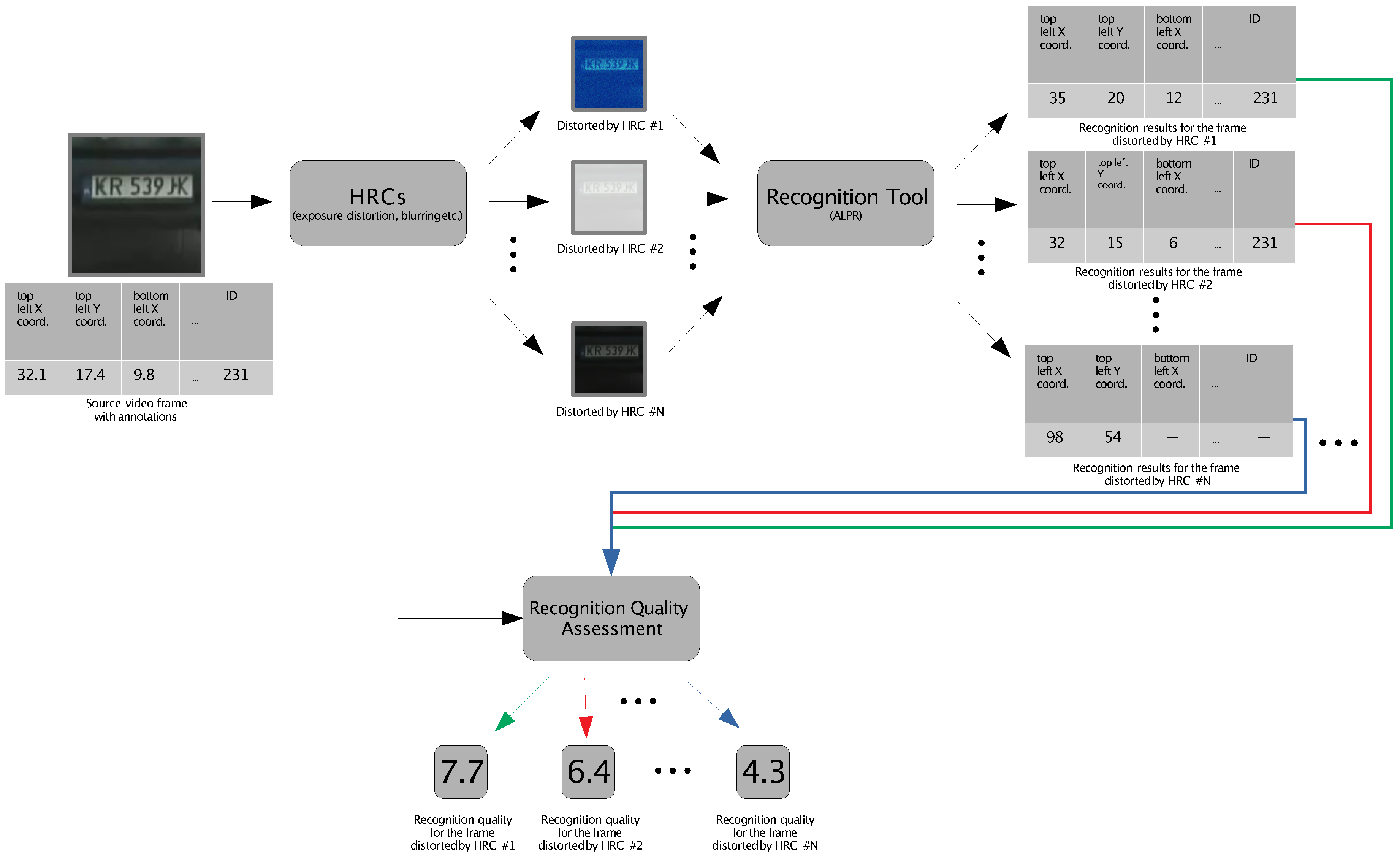
This experiment concentrates on single video frames, barring the Temporal Activity (TA) Video Quality Indicator (VQI). The application of a set of VQIs yields a vector of outcomes, with each VQI generating a distinct result. A detailed workflow is illustrated in Figure 16, adapted from Leszczuk et al. [2]. These findings are merged with those from the recognition test to produce input data for modeling.

The choice of programming language varies depending on the specific Video Quality Indicator (VQI) being utilized. For some VQIs, we employ C/C++ code, while for others, MATLAB code is used.

In order to streamline the execution of the experiment, we encapsulate all necessary components within a Python script. This script is designed to receive a list of filenames as input, allowing us to process a sizable batch of video frames simultaneously.

The quality experiment is just one of several software modules used in our workflow. All of these modules are controlled by a central Python script, known as the “master script”. As a result, the script employed in this particular experiment can generate its results either in the form of a JSON file or as a Python return value. An example of a JSON output file is provided in Listing 2.

Listing 2. An exemplary output JSON file, as produced by the Python script (performing the quality experiment).

2.4.2. Indicators

We selected a total of 19 VQIs based on their potential effectiveness and computational requirements.

Our AGH Video Quality (VQ) team provided eleven (11) of these VQIs (they can be downloaded from the link provided in Section “Supplementary Materials”):

• AGH:
  • Commercial Black: An indicator that measures the level of black coloration in commercial content;
  • Blockiness [2,21]: Refers to the visual artifacts caused by block-based coding schemes, often seen as grid-like structures in the image or video;
  • Block Loss [22]: Measures the instances where data blocks are lost during transmission or encoding, leading to visual corruption;
  • Blur [1,2,21]: Quantifies the loss of edge sharpness in an image or video, leading to a less clear representation;
  • Contrast: An indicator of the difference in luminance or color that makes objects in an image distinguishable;
  • Exposure [2]: Evaluates the balance of light in a photo or video, indicating over-exposure or under-exposure;
  • Interlacing [23]: Relates to the visual artifacts arising from interlaced scanning methods in video, usually observed as a flickering effect;
  • Noise [23]: Measures the amount of random visual static in an image or video, often arising from sensor or transmission errors;
  • Slice [22]: Assesses the impact of slice loss, which refers to the loss of a data segment that leads to noticeable visual errors;
  • Spatial Activity [2,21]: Measures the level of detail or texture in a still image or in each frame of a video;
  • Temporal Activity [2,21]: Gauges the rate of change between frames in a video, usually related to the amount of motion or action.

The remaining eight (8) VQIs are provided by external laboratories:

• LIVE:

  12.

  BIQI [24]: A Blind Image Quality Index that provides a quality score without referencing the original image;

  13.

  BRISQUE [25]: The Blind/Reference-less Image Spatial Quality Evaluator, which aims to assess the quality of images without a reference image;

  14.

  NIQE [26]: The Naturalness Image Quality Evaluator evaluates the perceptual quality of an image in a completely blind manner;

  15.

  OG-IQA [27]: Object Geometric-Based Image Quality Assessment focuses on evaluating the image quality based on geometric distortions;

  16.

  FFRIQUEE [28]: A Free-Energy-based Fractal Reference-less Image Quality Evaluator that operates without needing a reference image;

  17.

  IL-NIQE [29]: The Information-theoretic Local Naturalness Image Quality Evaluator uses local image statistics for the quality assessment;

• UMIACS:

  18.

  CORNIA [30]: The Codebook Representation for No-Reference Image Assessment evaluates the quality of images using a learned codebook representation;

• BUPT:

  19.

  HOSA [31]: The Higher-Order Statistics Aggregation for Blind Image Quality Assessment employs higher-order statistics to evaluate image quality.

The selection of MATLAB or C/C++ code depends on the specific VQI being utilized. The rationale behind the selection and omission of certain VQIs is detailed in the supplementary material section.

Table 3. List of Video Quality Indicators (VQIs) employed in the quality assessment experiment (source: [2]).

No	Name	Authors	Language
1	Commercial Black	VQ AGH	C/C++
2	Blockiness * [2,21]		C/C++
3	Block Loss * [22]		C/C++
4	Blur [1,2,21]		C/C++
5	Contrast		C/C++
6	Exposure [2]		C/C++
7	Interlacing [23]		C/C++
8	Noise [23]		C/C++
9	Slicing [22]		C/C++
10	Spatial Activity [2,21]		C/C++
11	Temporal Activity [2,21]		C/C++
12	BIQI [24]	LIVE	MATLAB
13	BRISQUE [25]		MATLAB
14	NIQE [26]		MATLAB
15	OG-IQA [27]		MATLAB
16	FFRIQUEE [28]		MATLAB
17	IL-NIQE [29]		MATLAB
18	CORNIA [30]	UMIACS	MATLAB
19	HOSA [31]	BUPT	MATLAB

presents a comprehensive list of all employed VQIs, accompanied by their descriptions and relevant references. The indicators highlighted with an asterisk (*) may not directly correlate with the precise objectives of the investigation, but they are included due to their potential value during the modeling stage. Additionally, their inclusion does not significantly impact the computation time overhead. UMIACS and BUPT are the initials for the University of Maryland Institute for Advanced Computer Studies (Language and Media Processing Laboratory) and the Beijing University of Posts and Telecommunications (School of Information and Communication Engineering, respectively.

During the preparatory phase of the experiment, we decided to exclude two measures, specifically (i) DIIVINE [32] and (ii) BLIINDS-II [33]. The removal of these indicators was due to their high computational demands, with BLIINDS-II requiring around 3 min to assess a single image’s quality. This exclusion was essential to maintain the experiment’s relevance concerning the quantity of Source Reference Codes (SRCs) that could be evaluated. Put simply, including DIIVINE and BLIINDS-II would significantly increase the duration of the experiment, rendering the assessment of a considerable number of SRCs impractical.

DIIVINE was excluded from the experiment in favor of a more refined alternative. We predict that FFRIQUEE will perform at least as well as DIIVINE. This assumption stems from the fact that FRIQUEE is built on the basis of DIIVINE.

In contrast, there is no alternative indication for BLIINDS-II at the moment. We chose to remove it, because it does not have the potential to outperform others. Based on existing research [34], we do not expect BLIINDS-II to be one of the best performing indicators.

2.4.3. VQI Execution Time

This subsection provides an empirical analysis of the time complexity of each VQI to help to determine the feasibility of a real-time assessment. As mentioned above, to determine the number of SRCs that can be tested, it is important to know the computational time required for all VQIs.

Table 4. Execution duration for each operational Video Quality Indicator (VQI). The total time for AGH VQIs represents the cumulative execution times of each VQI, as sourced from [21].

Algorithm Name	Duration [s]
BIQI	1.60
BRISQUE	1.67
NIQE	3.92
OG-IQA	5.72
FRIQUEE	40.79
IL-NIQE	10.70
CORNIA	7.71
HOSA	0.43
VQ AGH VQIs	0.12
Overall Total	72.66

presents a summary of the execution times for each VQI. It is important to note that these timings were recorded on a laptop featuring an Intel Core i7-3537U CPU.

2.4.4. Data as an Example

This section contains instances of collected data.

Finally, we present examples of the data to give a snapshot of the type of results that can be expected from this experiment. Various forms of distortion were applied to the video frames to simulate real-world conditions.

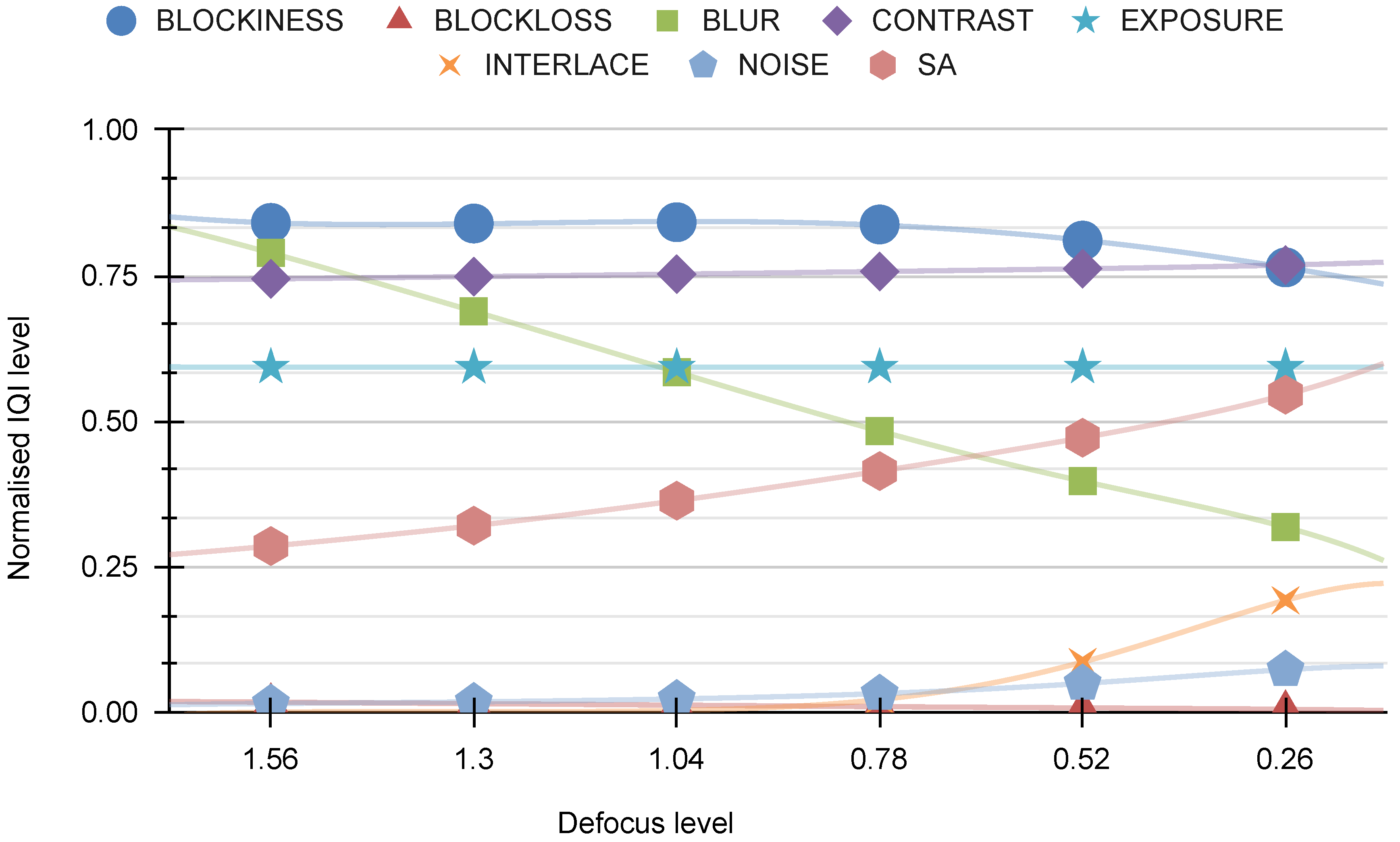
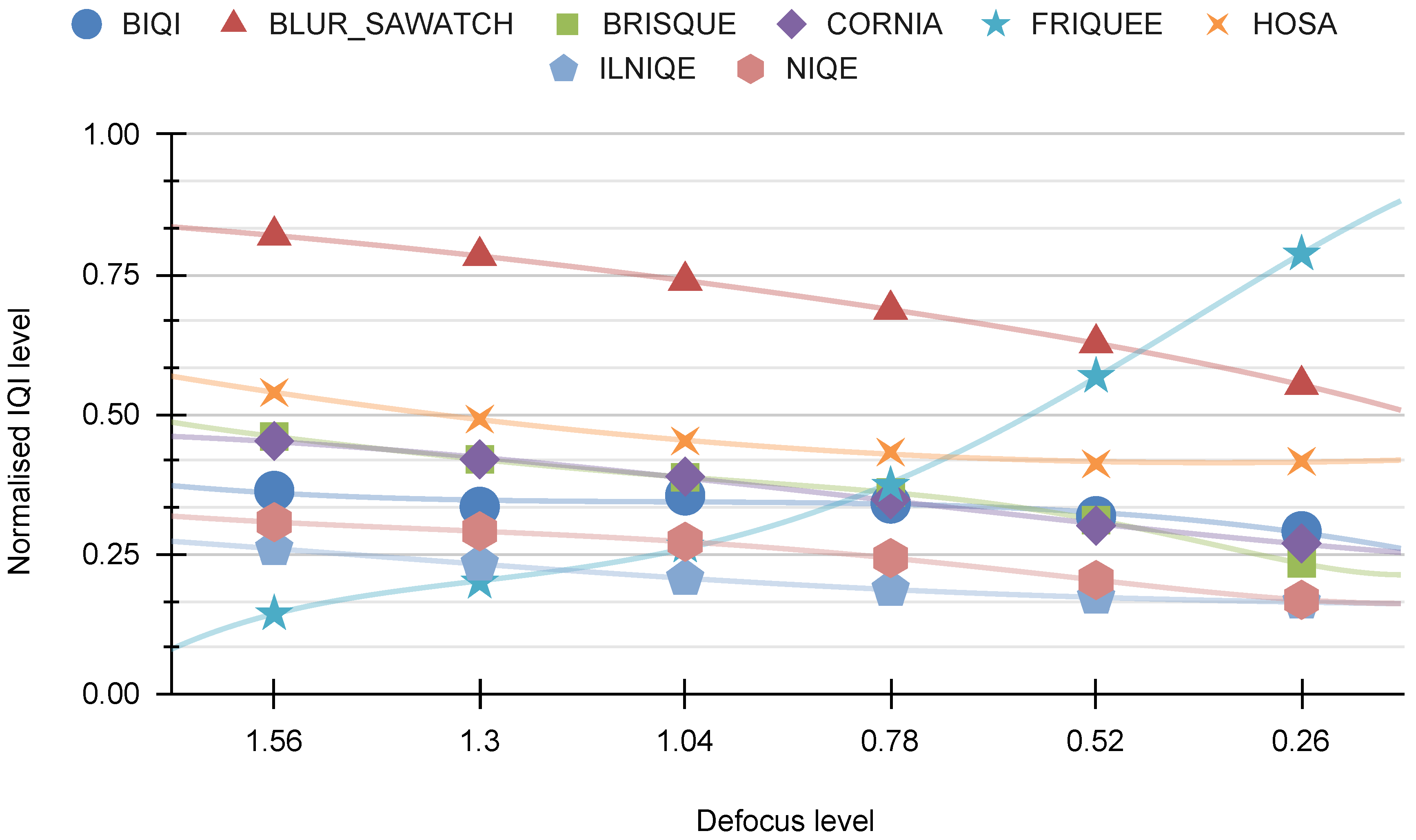
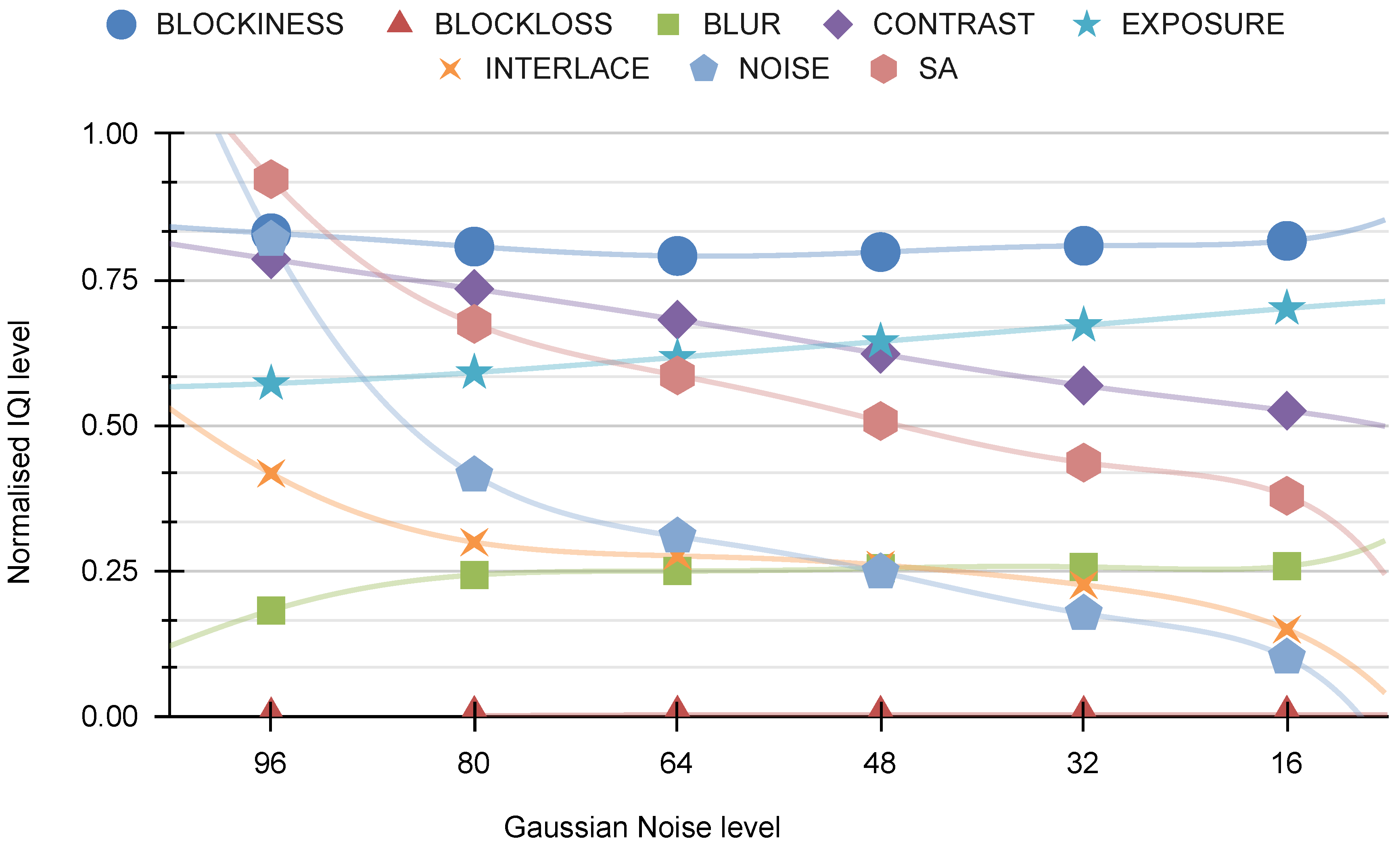
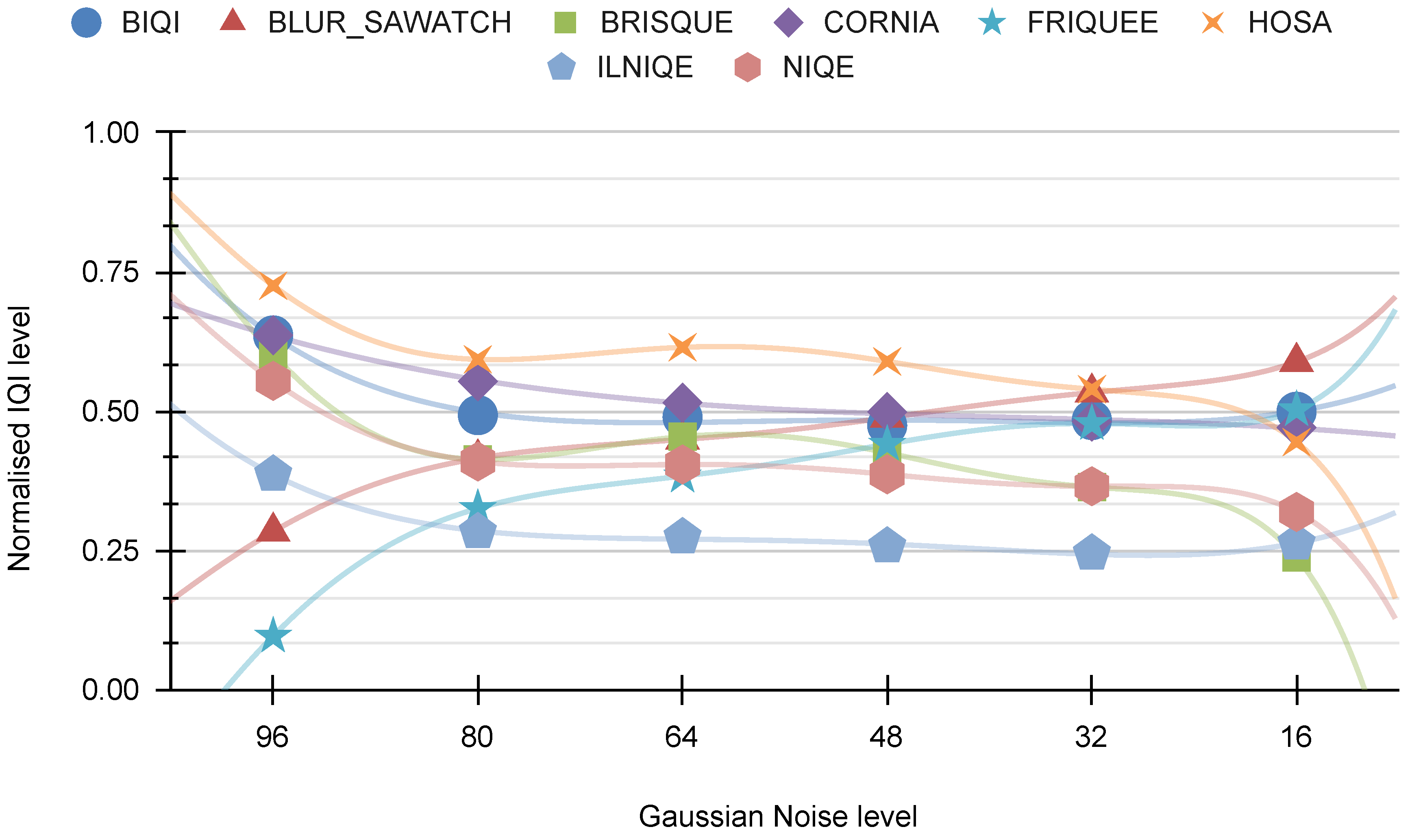
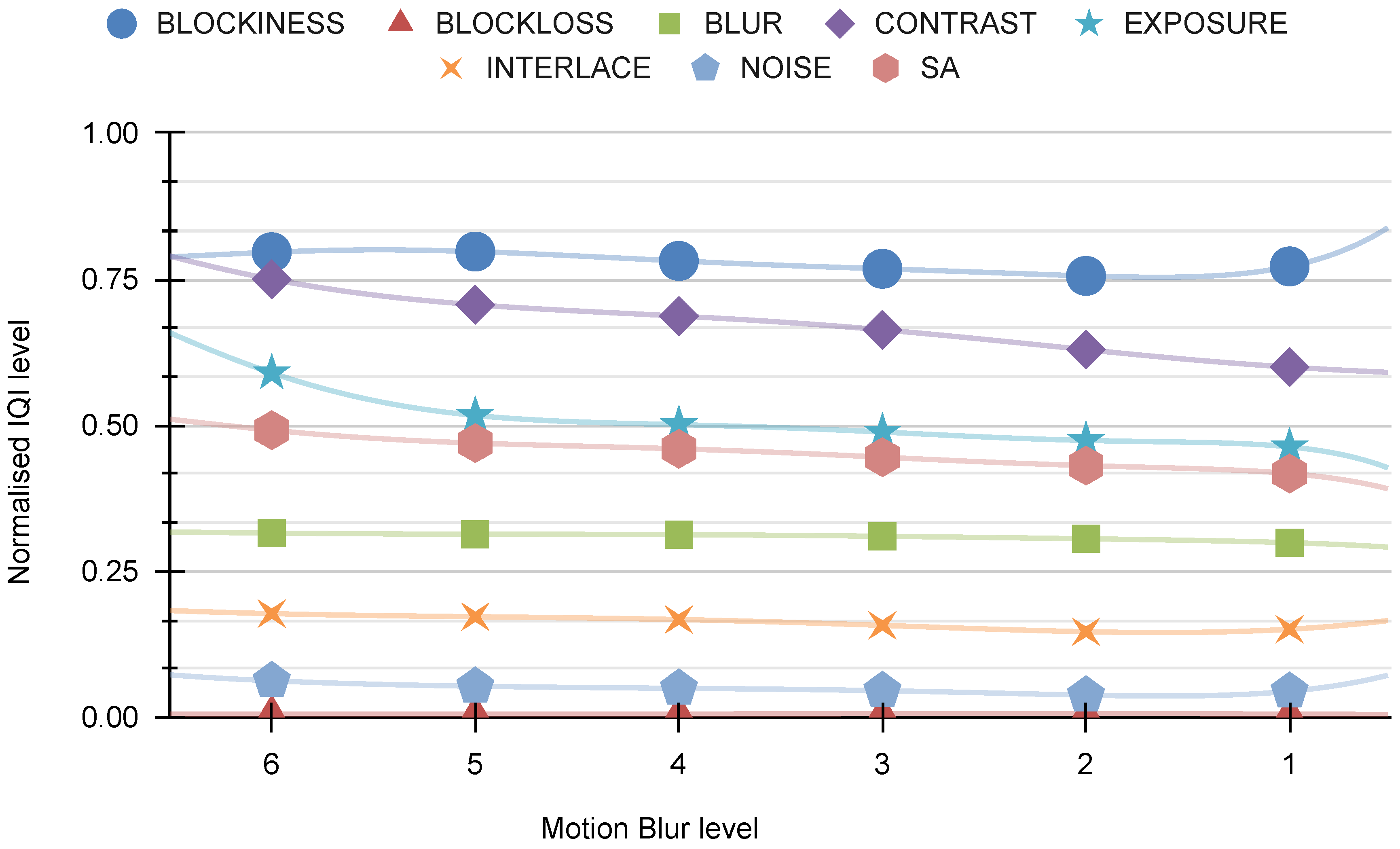
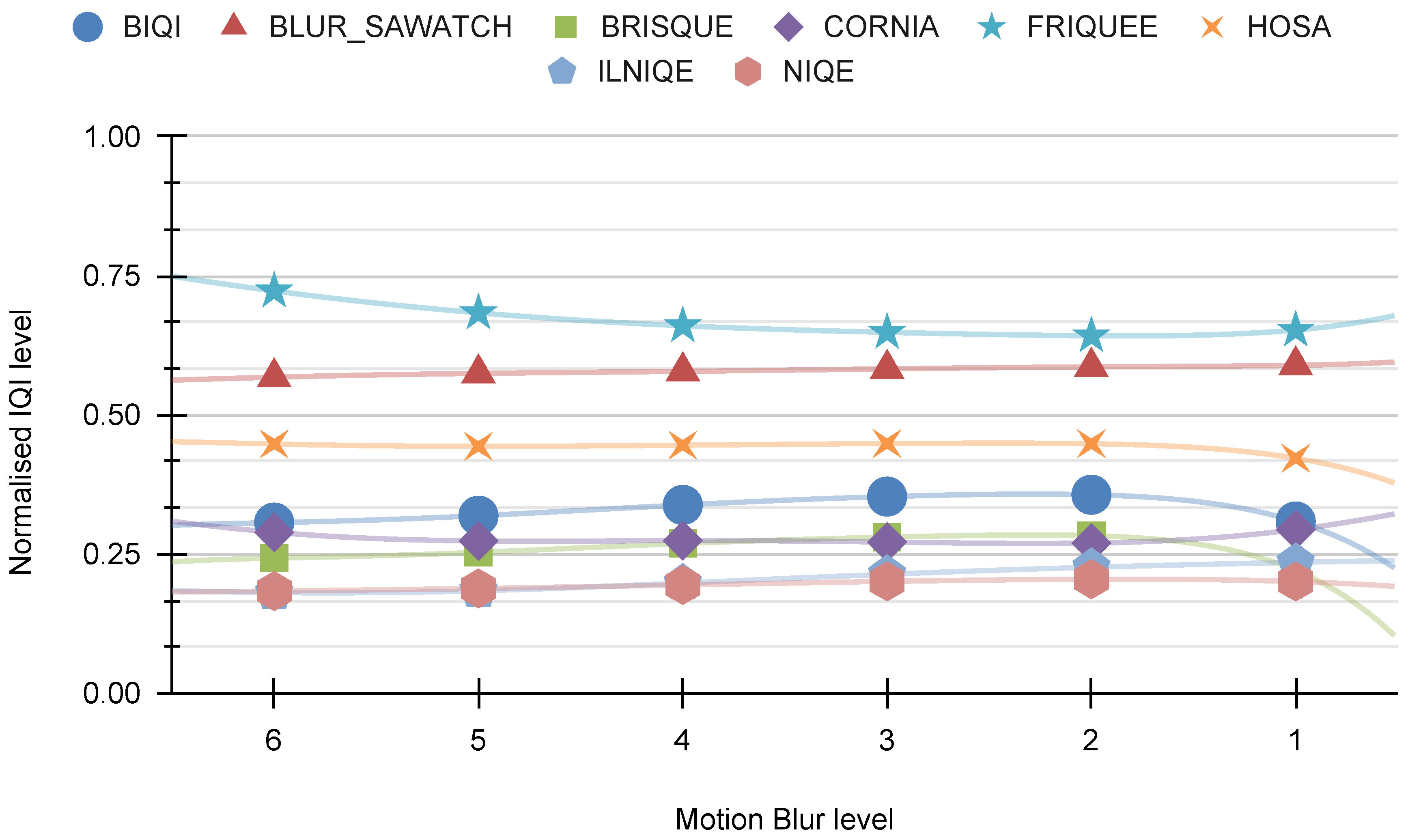
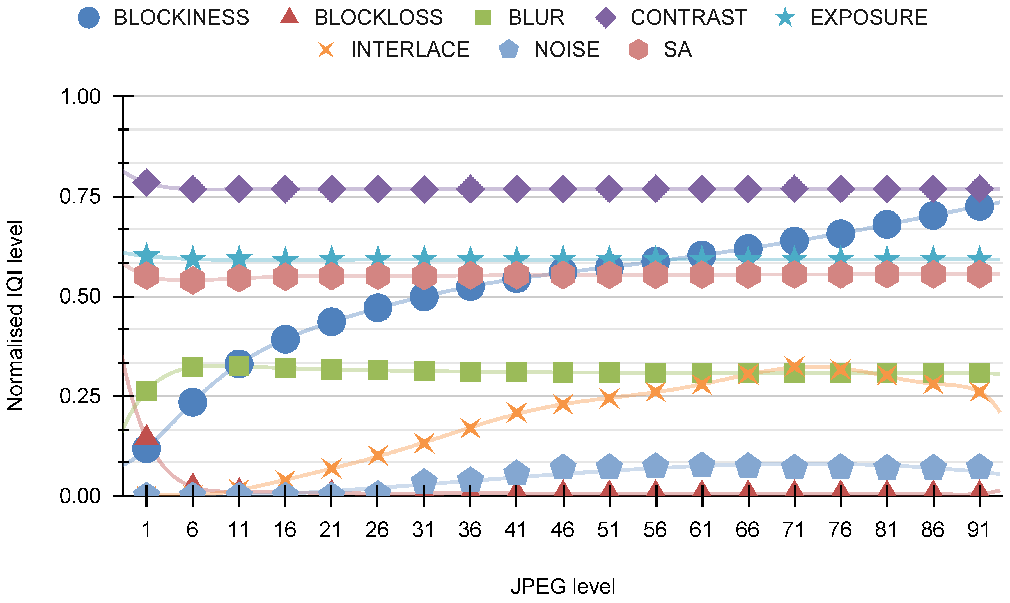
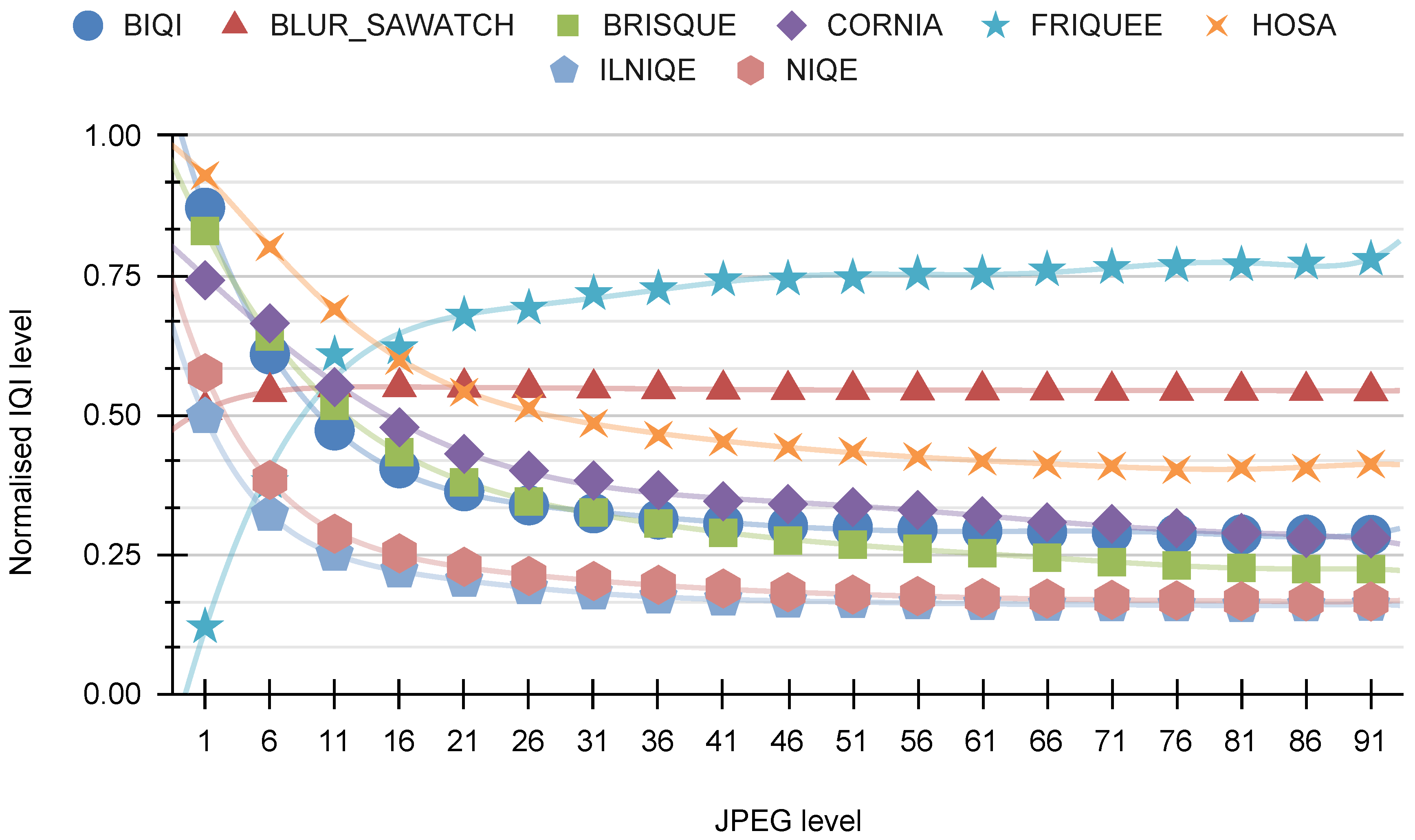
In the imaging process, we utilize four types of distortion (HRC): defocus, Gaussian noise, motion blur, and JPEG. For each HRC, two graphs are presented. The initial chart depicts eight representative visual indicators developed by our AGH team, including BLOCKINESS, BLOCK-LOSS, BLUR, CONTRAST, EXPOSURE, INTERLACE, NOISE, and SA. The subsequent graph illustrates eight visual indicators developed by various research groups: BIQI, BLUR-SAWATCH, CORNIA, FRIQUEE, HOSA, ILNIQE, and NIQE.

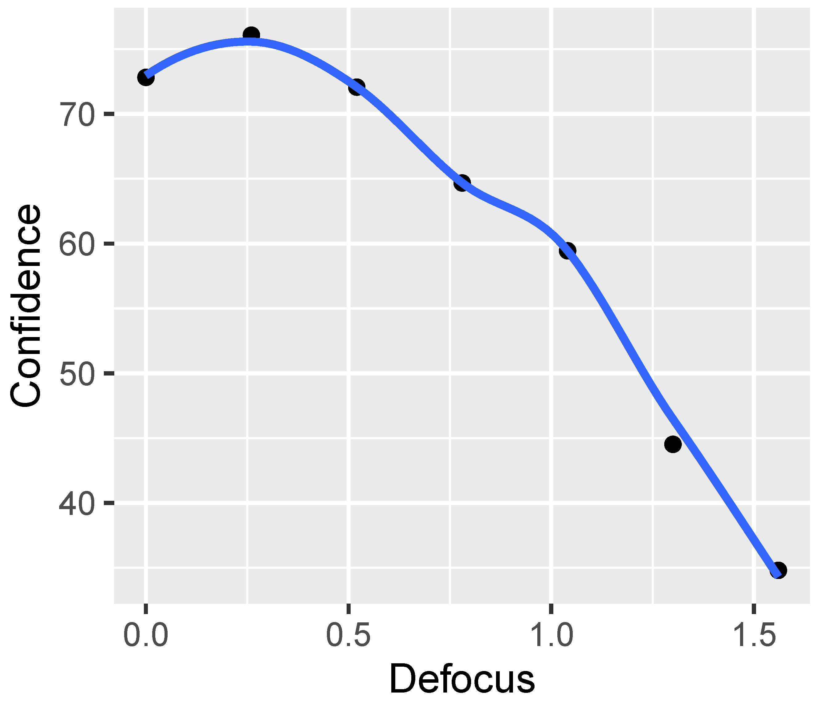
Figure 17 presents a comparative analysis of “our indicators” against defocus distortion. It is evident from the graph that this distortion significantly affects the BLUR indicator and has a somewhat lesser effect on the SA indicator.

The comparison between “other indications” and the defocus distortion is shown in Figure 18. It is evident from the chart that this distortion notably impacts the FRIQUEE and, to a lesser degree, the NIQE indicators.

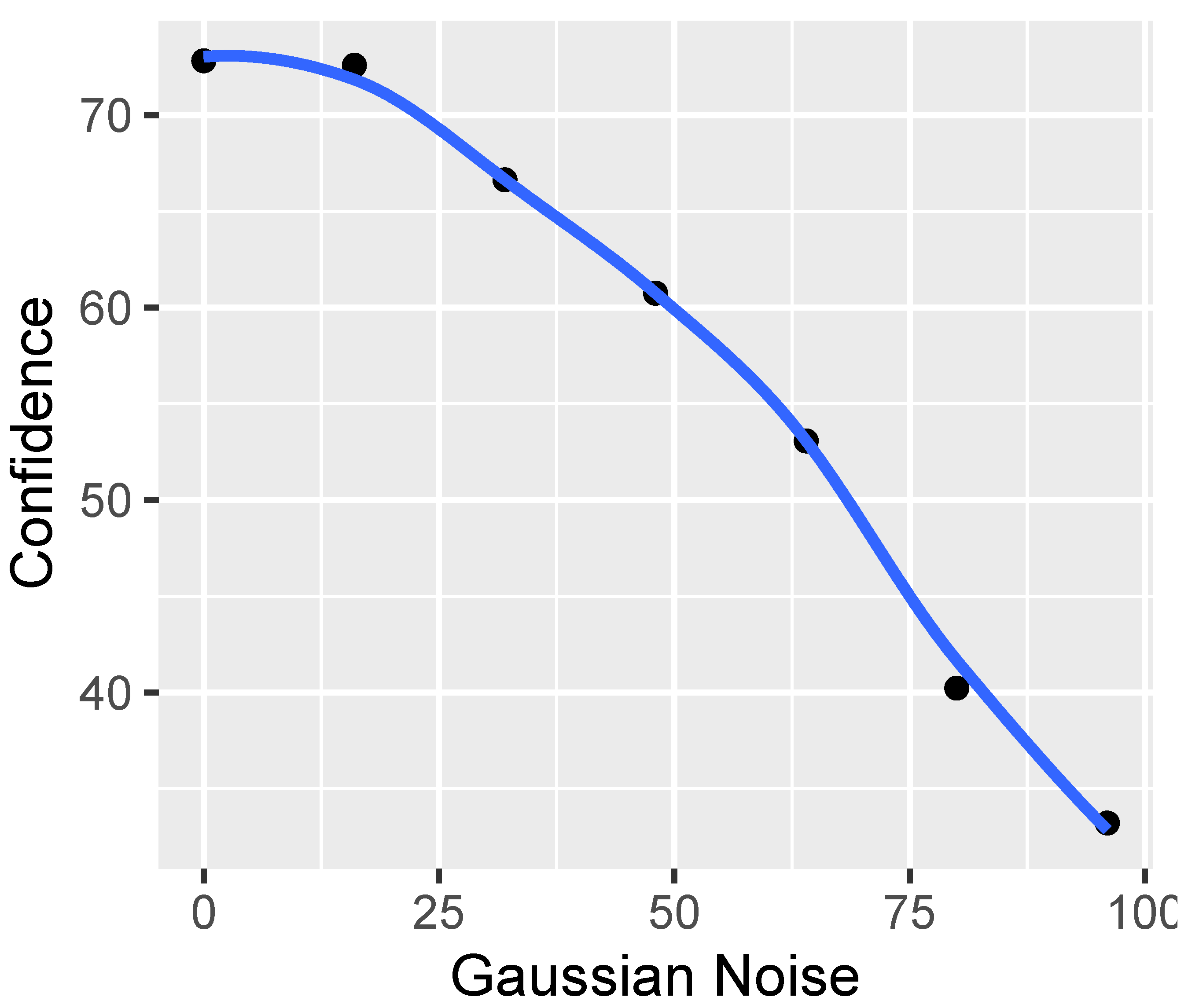
Figure 19 displays the correlation between “our indicators” and the Gaussian noise distortion. It is evident from the figure that this distortion primarily affects the NOISE indicator, with a minor impact on the SA indicator.

In Figure 20, the relationship between “other indicators” and Gaussian noise is depicted. This distortion evidently affects the FRIQUEE and NIQE indicators, and, to a more moderate extent, the BRISQUE indicator.

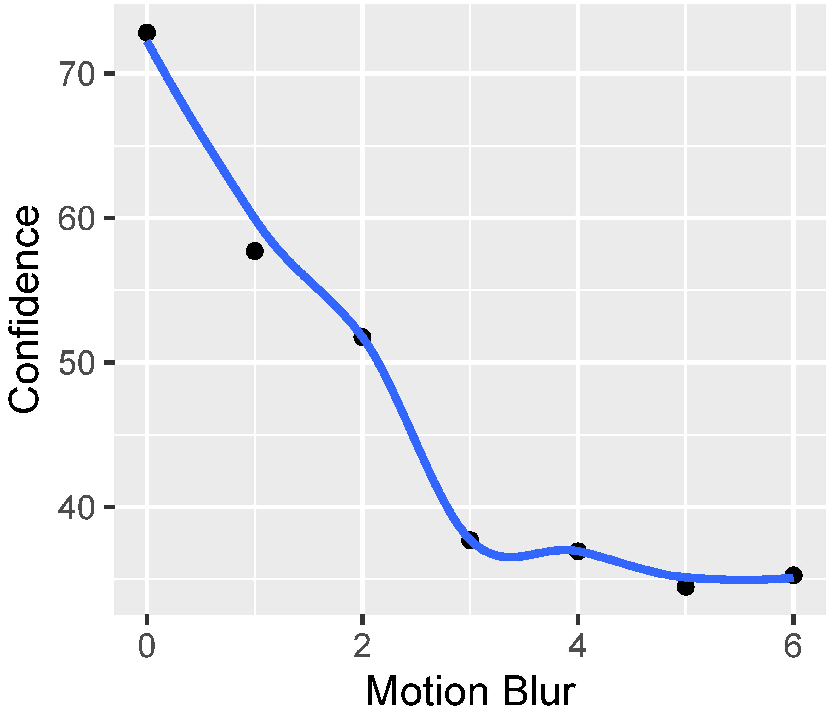
Figure 21 illustrates the relationship between “our indicators” and motion blur. It is discovered that this distortion has no discernible effect on any of the indicators.

Figure 22 depicts the relationship between “other indicators” and motion blur. The analysis reveals that this distortion does not have any noticeable impacts on any of the indicators.

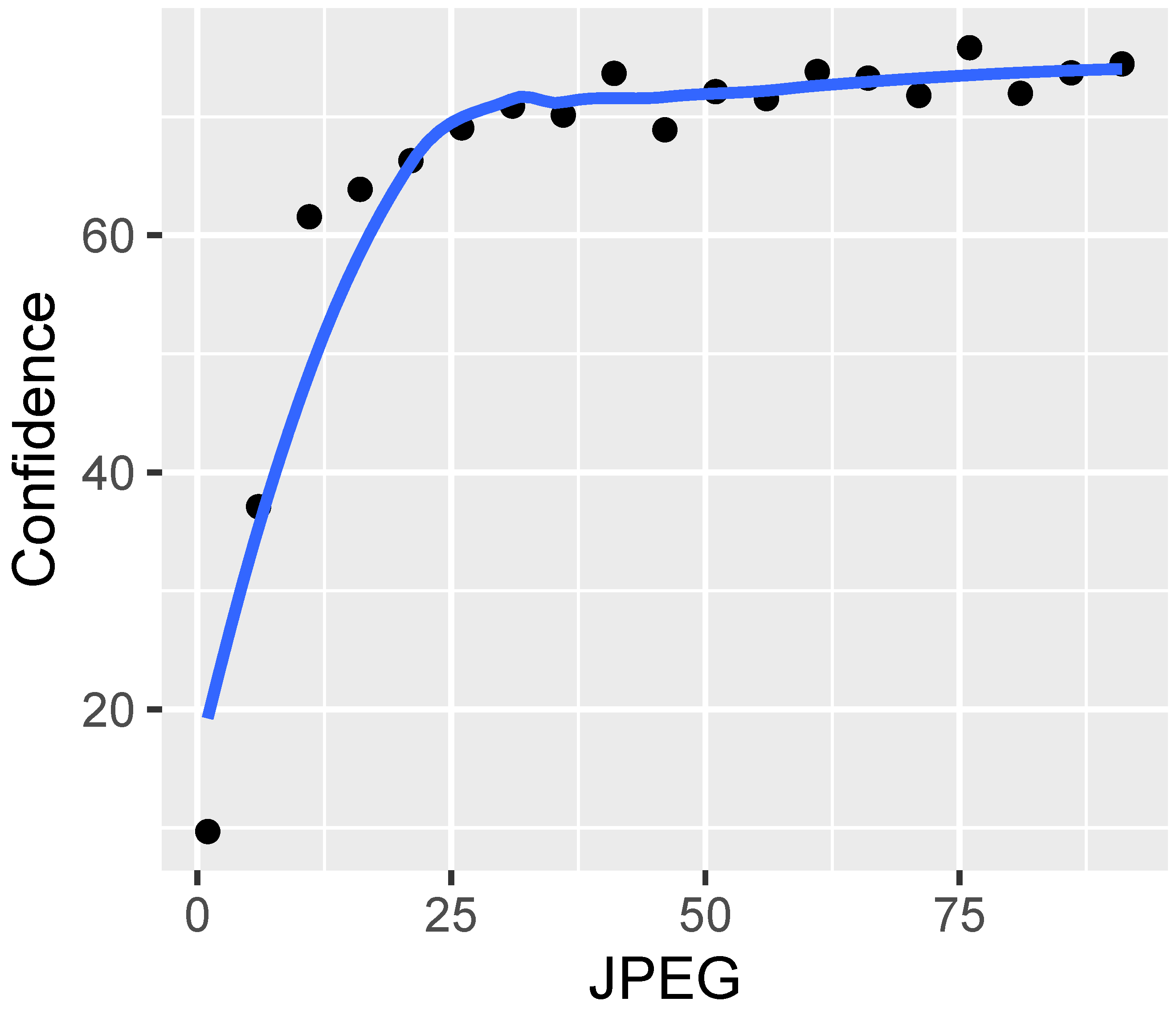
Figure 23 illustrates the correlation between “our indicators” and the distortion of the JPEG. It is evident that this distortion predominantly triggers a pronounced response in the BLOCKINESS indicator, which is expected, since this indicator is specifically designed for detecting JPEG artifacts.

Figure 24 shows the relationship between the “other indicators” and the JPEG distortion. This distortion clearly generates substantial responses from practically all indicators, particularly those in the lower range. However, the BLUR-SAWATCH indicator does not exhibit a strong response to JPEG distortion.

3. Results

This section outlines the results of developing a new objective video quality assessment model tailored for ALPR applications.

By leveraging data from both the quality and recognition experiments, models capable of forecasting recognition results based on VQIs can be constructed. This approach leads to the formation of a distinctive quality model. In particular, this model is applicable in situations where no particular target is defined for identification. Adaptations can be made to both the details of the recognition algorithm and the model itself.

We categorize the VQIs into two groups for modeling purposes. The first group, called “All metrics” includes both our own VQIs and those provided by other parties. The second group, called “only ours”, comprises only our own VQI.

In our analysis, we employ precision, recall, and the F-measure, which are common metrics in the domains of pattern recognition, information retrieval, and machine-learning-driven classification. Precision, also termed a positive predictive value, indicates the proportion of correct instances among the retrieved cases. Recall, or sensitivity, reflects the proportion of all pertinent instances that are accurately identified. Both precision and recall are rooted in the notion of relevance. The F-measure, being the harmonic mean of precision and recall, merges these metrics into a singular measure, offering a comprehensive evaluation of performance [35].

Among the various modeling approaches used for the ALPR system, decision trees emerged as the most effective method.

We considered two classification scenarios for this ALPR system: binary classification, where the classes are “license plate recognized” and “license plate not recognized”, and multiclass classification, where the classes are “license plate recognized”, “license plate recognized with one error”, “license plate recognized with two errors”, “license plate recognized with three errors” and “license plate not recognized”.

We obtained the results for two classes, as delineated in

Table 5. General results received for ALPR for two classes (source: [2]).

	Precision	Recall	F-Measure
All metrics	0.779	0.776	0.777
Only ours	0.758	0.759	0.764

. Each column in the table represents a specific metric used to evaluate the model’s performance. Specifically, the column labeled “F-measure” represents the F1 score, providing a balanced measure of the accuracy and completeness of a model. This F-measure parameter has a value of 0.777 for the “All metrics” row, indicating the model’s performance when considering all metrics together. For further details on how each metric is calculated, the reader can refer to the following link: https://scikit-learn.org/stable/modules/generated/sklearn.metrics.precision_recall_fscore_support.html (accessed on 14 November 2023).

We obtained results for five classes, which are presented in

Table 6. The general results received for ALPR for five classes (source: [2]).

	Precision	Recall	F-Measure
All metrics	0.415	0.425	0.407
Only ours	0.401	0.405	0.394

.

The outcomes for the test set are notably inferior, even when considering the suboptimal results for the validation set. The key reason for this difference is the substantial influence of the source, which seems to exert a greater effect than the distortion itself. In terms of cognitive thinking, this means that letters such as “D” and “O” are more likely to be misidentified than other more distinct letters such as “K”.

The evaluation results of the model, which is designed to handle two distinct classes and includes a comprehensive set of performance metrics, reveal that its overall performance is not up to the mark when subjected to tests on the test set. Specifically, the model’s capability for accurately detecting the correct classes falls short, with an estimated success rate of approximately two-thirds. This is corroborated by the data presented in

Table 7. Confusion matrix for the test set, ALPR scenario, all metrics, and two classes (source: [2]).

			Algorithm
		Not more than 2 errors	Other cases
Truth	Not more than 2 errors	292	302
	Other cases	138	628

and

Table 8. Performance parameters for the test set, ALPR scenario, all metrics, and two classes (source: [2]).

	Precision	Recall	F-Measure	Support
Not more than 2 errors	0.679	0.492	0.570	594
Other cases	0.675	0.820	0.741	766
Macro average	0.677	0.656	0.655	1360
Weighted average	0.677	0.676	0.666	1360

, which provide a detailed breakdown of these performance metrics.

The performance evaluation of the model, which is configured to categorize data into five distinct classes and incorporates a comprehensive suite of metrics for assessment, shows that it achieves particularly strong results on the test set, especially for the two primary classes. This outcome is generally expected, given that these two classes contain the largest number of instances within the dataset. In addition to excelling in the classification of the two main classes, the model also shows a satisfactory level of accuracy when it comes to identifying instances where no license plate is detected. These evaluations and conclusions are supported by the information displayed in

Table 9. Confusion matrix for the test set, ALPR scenario, all metrics, and five classes (source: [2]).

						Algorithm
		Correct recogn.	1 error	2 errors	3+ errors	No detection
Truth	Correct recogn.	190	30	21	6	29
	1 error	109	48	14	11	43
	2 errors	22	24	14	4	29
	3+ errors	25	16	6	6	43
	No detection	101	102	12	23	432

and

Table 10. Performance parameters for the test set, ALPR scenario, all metrics, and five classes (source: [2]).

	Precision	Recall	F-Measure	Support
Correct recognition	0.425	0.688	0.526	276
1 error	0.218	0.213	0.216	225
2 errors	0.209	0.151	0.175	93
3+ errors	0.120	0.062	0.082	96
No detection	0.750	0.645	0.693	670
Macro average	0.344	0.352	0.338	1360
Weighted average	0.515	0.507	0.502	1360

, where a more detailed analysis of performance metrics is available.

The performance of the two-class model using AGH metrics closely mirrors the results observed across all classes, as depicted in

Table 11. Confusion matrix for the test set, ALPR scenario, our metrics, and two classes (source: [2]).

			Algorithm
		Not more than 2 errors	Other cases
Truth	Not more than 2 errors	232	362
	Other cases	118	648

and

Table 12. Performance parameters for the test set, ALPR scenario, our metrics, and two classes (source: [2]).

	Precision	Recall	F-Measure	Support
Not more than 2 errors	0.663	0.391	0.492	594
Other cases	0.642	0.846	0.730	766
Macro average	0.652	0.618	0.611	1360
Weighted average	0.651	0.647	0.626	1360

.

The results of the five-class model using AGH metrics again show a similarity to the results acquired for all metrics, as illustrated in

Table 13. Confusion matrix for the test set, ALPR scenario, our metrics, and five classes (source: [2]).

						Algorithm
		Correct recogn.	1 error	2 errors	3+ errors	No detection
Truth	Correct recogn.	165	40	13	12	46
	1 error	102	40	18	9	56
	2 errors	27	18	16	5	27
	3+ errors	21	8	12	11	44
	No detection	138	50	31	25	426

and

Table 14. Performance parameters for the test set, ALPR scenario, our metrics, and five classes (source: [2]).

	Precision	Recall	F-Measure	Support
Correct recognition	0.364	0.598	0.453	276
1 error	0.256	0.178	0.210	225
2 errors	0.178	0.172	0.175	93
3+ errors	0.177	0.115	0.139	96
No detection	0.711	0.636	0.671	670
Macro average	0.337	0.340	0.330	1360
Weighted average	0.491	0.484	0.479	1360

.

The numerical study sought to determine the susceptibility of the model to various distortions. As demonstrated in Figure 25, the model displayed a consistent error sensitivity in several types of HRC. The error rates for Gaussian noise, defocus, motion blur, and JPEG compression were relatively similar, with percentages hovering around the thirty percent mark.

On the contrary, the model showed a considerably lower error rate for the HRC exposure, only 11%. This suggests that the model is significantly more robust to variations in exposure than to other distortions tested. On the other hand, the JPEG HRC resulted in a higher error rate than expected, which is a point of interest and could be explored further in future work.

4. Conclusions

In closing, this work addresses the gap identified in the Introduction by providing an objective evaluation methodology for TRVs, with a specific focus on ALPR systems under challenging conditions. The validity of the methodology is evidenced by an F-measure of 0.777, confirming the predictive power of our system under diverse scenarios. This reflects the fulfillment of our aim of constructing models that accurately predict the utility of TRVs in various applications.

We have presented a comprehensive dataset and an assessment system, which offers significant contributions to both academic and industrial spheres in the domain of the TRVs. These efforts extend the scope of traditional quality metrics, underscoring the importance of specialized evaluations for recognition tasks which traditional metrics overlook. Although the limitations of our current model, specific to ALPR tasks, are noted, the F-measure of 0.764, despite AGH VQI restrictions, suggests strong potential for broader application.

The initial scene qualities play a pivotal role in the recognition accuracy and present a challenge for current VQIs, which our future work will aim to address. Adhering to the foundations laid out in this paper, our subsequent research will expand the applicability of our model to encompass a wider range of conditions and recognition systems.

Prospective research will focus on refining the JND threshold to enhance the CV performance, with the aim of developing a lossless quality model. This model will be subjected to an extensive set of CV algorithms and a variety of image distortions. Through these efforts, we aim to establish a robust framework that can predict lossless CV performance, accelerating advances in high-precision recognition systems [2].

References

1. Leszczuk, M. Revising and Improving the ITU-T Recommendation P. 912. J. Telecommun. Inf. Technol. 2015, 1, 10–14. [Google Scholar]
2. Leszczuk, M.; Janowski, L.; Nawała, J.; Boev, A. Method for Assessing Objective Video Quality for Automatic License Plate Recognition Tasks. In Proceedings of the Multimedia Communications, Services and Security: 11th International Conference, MCSS 2022, Kraków, Poland, 3–4 November 2022; Springer International Publishing: Cham, Switzerland, 2022; pp. 153–166. [Google Scholar]
3. Shi, H.; Liu, C. An Innovative Video Quality Assessment Method and An Impairment Video Dataset. In Proceedings of the 2021 IEEE International Conference on Imaging Systems and Techniques (IST), Kaohsiung, Taiwan, 24–26 August 2021; pp. 1–6. [Google Scholar]
4. Xing, W.; Lyu, T.; Chu, X.; Rong, Y.; Lee, C.G.; Sun, Q.; Zou, Y. Recognition and classification of single melt tracks using deep neural network: A fast and effective method to determine process windows in selective laser melting. J. Manuf. Process. 2021, 68, 1746–1757. [Google Scholar] [CrossRef]
5. Khan, Z.A.; Beghdadi, A.; Cheikh, F.A.; Kaaniche, M.; Pelanis, E.; Palomar, R.; Fretland, Å.A.; Edwin, B.; Elle, O.J. Towards a video quality assessment based framework for enhancement of laparoscopic videos. In Proceedings of the Medical Imaging 2020: Image Perception, Observer Performance, and Technology Assessment, Houston, TX, USA, 16 March 2020; Volume 11316. [Google Scholar]
6. Hofbauer, H.; Autrusseau, F.; Uhl, A. To recognize or not to recognize–A database of encrypted images with subjective recognition ground truth. Inf. Sci. 2021, 551, 128–145. [Google Scholar] [CrossRef]
7. Wu, J.; Ma, J.; Liang, F.; Dong, W.; Shi, G.; Lin, W. End-to-end blind image quality prediction with cascaded deep neural network. IEEE Trans. Image Process. 2020, 29, 7414–7426. [Google Scholar] [CrossRef]
8. Oszust, M. Local feature descriptor and derivative filters for blind image quality assessment. IEEE Signal Process. Lett. 2019, 26, 322–326. [Google Scholar] [CrossRef]
9. Mahankali, N.S.; Raghavan, M.; Channappayya, S.S. No-Reference Video Quality Assessment Using Voxel-wise fMRI Models of the Visual Cortex. IEEE Signal Process. Lett. 2021, 29, 319–323. [Google Scholar] [CrossRef]
10. Hosu, V.; Hahn, F.; Jenadeleh, M.; Lin, H.; Men, H.; Szirányi, T.; Li, S.; Saupe, D. The Konstanz natural video database (KoNViD-1k). In Proceedings of the 2017 Ninth International Conference on Quality of Multimedia Experience (QoMEX), Erfurt, Germany, 31 May–2 June 2017; pp. 1–6. [Google Scholar]
11. Sinno, Z.; Bovik, A.C. Large-scale study of perceptual video quality. IEEE Trans. Image Process. 2018, 28, 612–627. [Google Scholar] [CrossRef]
12. Wang, Y.; Inguva, S.; Adsumilli, B. YouTube UGC dataset for video compression research. In Proceedings of the 2019 IEEE 21st International Workshop on Multimedia Signal Processing (MMSP), Kuala Lumpur, Malaysia, 27–29 September 2019; pp. 1–5. [Google Scholar]
13. Ying, Z.; Mandal, M.; Ghadiyaram, D.; Bovik, A. Patch-VQ: ‘Patching Up’ the video quality problem. In Proceedings of the IEEE/CVF Conference on Computer Vision and Pattern Recognition, Nashville, TN, USA, 20–25 June 2021; pp. 14019–14029. [Google Scholar]
14. FFmpeg. 2019. Available online: https://ffmpeg.org/ (accessed on 4 June 2019).
15. ImageMagick Studio LLC. ImageMagick: Convert, Edit, or Compose Bitmap Images. 2011. Available online: https://imagemagick.org/script/cite.php (accessed on 23 May 2019).
16. Wikipedia. Exposure (Photography)—Wikipedia, The Free Encyclopedia. 2019. Available online: http://en.wikipedia.org/w/index.php?title=Exposure%20(photography)&oldid=897791540 (accessed on 23 May 2019).
17. Wikipedia. Defocus Aberration—Wikipedia, The Free Encyclopedia. 2019. Available online: http://en.wikipedia.org/w/index.php?title=Defocus%20aberration&oldid=886641679 (accessed on 23 May 2019).
18. Wikipedia. Gaussian Noise—Wikipedia, The Free Encyclopedia. 2019. Available online: http://en.wikipedia.org/w/index.php?title=Gaussian%20noise&oldid=886816599 (accessed on 23 May 2019).
19. Wikipedia. Motion Blur—Wikipedia, The Free Encyclopedia. 2019. Available online: http://en.wikipedia.org/w/index.php?title=Motion%20blur&oldid=896903005 (accessed on 23 May 2019).
20. Wikipedia. JPEG—Wikipedia, The Free Encyclopedia. 2021. Available online: https://en.wikipedia.org/w/index.php?title=JPEG&oldid=1061886975 (accessed on 25 December 2021).
21. Nawała, J.; Leszczuk, M.; Zajdel, M.; Baran, R. Software package for measurement of quality indicators working in no-reference model. Multimed. Tools Appl. 2016, 1–17. [Google Scholar] [CrossRef]
22. Leszczuk, M.; Hanusiak, M.; Farias, M.C.; Wyckens, E.; Heston, G. Recent developments in visual quality monitoring by key performance indicators. Multimed. Tools Appl. 2016, 75, 10745–10767. [Google Scholar] [CrossRef]
23. Schatz, R.; Hoßfeld, T.; Janowski, L.; Egger, S. From packets to people: Quality of experience as a new measurement challenge. Data Traffic Monit. Anal. Meas. Classif. Anom. Detect. Qual. Exp. 2013, 7754, 219–263. [Google Scholar]
24. Xue, W.; Mou, X.; Zhang, L.; Bovik, A.C.; Feng, X. Blind image quality assessment using joint statistics of gradient magnitude and Laplacian features. IEEE Trans. Image Process. 2014, 23, 4850–4862. [Google Scholar] [CrossRef]
25. Mittal, A.; Moorthy, A.K.; Bovik, A.C. No-reference image quality assessment in the spatial domain. IEEE Trans. Image Process. 2012, 21, 4695–4708. [Google Scholar] [CrossRef]
26. Yang, C.; He, Q.; An, P. Unsupervised blind image quality assessment via joint spatial and transform features. Sci. Rep. 2023, 13, 10865. [Google Scholar] [CrossRef]
27. Liu, L.; Hua, Y.; Zhao, Q.; Huang, H.; Bovik, A.C. Blind image quality assessment by relative gradient statistics and adaboosting neural network. Signal Process. Image Commun. 2016, 40, 1–15. [Google Scholar] [CrossRef]
28. Ghadiyaram, D.; Bovik, A.C. Perceptual quality prediction on authentically distorted images using a bag of features approach. J. Vis. 2017, 17, 32. [Google Scholar] [CrossRef]
29. Zhang, L.; Zhang, L.; Bovik, A.C. A feature-enriched completely blind image quality evaluator. IEEE Trans. Image Process. 2015, 24, 2579–2591. [Google Scholar] [CrossRef]
30. Ye, P.; Kumar, J.; Kang, L.; Doermann, D. Unsupervised feature learning framework for no-reference image quality assessment. In Proceedings of the 2012 IEEE Conference on Computer Vision and Pattern Recognition, Providence, RI, USA, 16–21 June 2012; pp. 1098–1105. [Google Scholar]
31. Xu, J.; Ye, P.; Li, Q.; Du, H.; Liu, Y.; Doermann, D. Blind image quality assessment based on high order statistics aggregation. IEEE Trans. Image Process. 2016, 25, 4444–4457. [Google Scholar] [CrossRef]
32. Gao, X.; Gao, F.; Tao, D.; Li, X. Universal blind image quality assessment metrics via natural scene statistics and multiple kernel learning. IEEE Trans. Neural Netw. Learn. Syst. 2013, 24, 2013–2026. [Google Scholar]
33. Saad, M.A.; Bovik, A.C.; Charrier, C. Blind image quality assessment: A natural scene statistics approach in the DCT domain. IEEE Trans. Image Process. 2012, 21, 3339–3352. [Google Scholar] [CrossRef]
34. Lin, H.; Hosu, V.; Saupe, D. KonIQ-10K: Towards an ecologically valid and large-scale IQA database. arXiv 2018, arXiv:1803.08489. [Google Scholar]
35. Wikipedia. Precision and Recall—Wikipedia, The Free Encyclopedia. 2020. Available online: https://en.wikipedia.org/w/index.php?title=Precision_and_recall&oldid=965503278 (accessed on 6 July 2020).
Figure 1. General methodology flow chart outlining the interactions among the recognition experiment, quality experiment, and the objective video quality assessment model.
Electronics 12 04721 g001
Figure 2. Sample image from the AGH collection, utilized for evaluating the video quality in the context of license plate identification.
Electronics 12 04721 g002
Figure 3. An assembled display of the chosen SRC images for the purpose of ALPR.
Electronics 12 04721 g003
Figure 4. A diagrammatic representation of a single-lens reflex camera, annotated with basic labels in accordance with standard reflex camera nomenclature. Jean François WITZ created the original foundation picture. According to Astrocog—Original work, CC BY-SA 3.0, https://commons.wikimedia.org/w/index.php?curid=29334470 (accessed on 14 November 2023).
Electronics 12 04721 g004
Figure 5. A diagram of a pinhole camera. By en:User:DrBob (original); en:User:Pbroks13 (redraw)—http://commons.wikimedia.org/wiki/Image:Pinhole-camera.png (accessed on 14 November 2023), Public Domain, https://commons.wikimedia.org/w/index.php?curid=4099853 (accessed on 14 November 2023).
Electronics 12 04721 g005
Figure 6. Schematicrepresentation of the distortion model illustrating the conversion of luminous flux from the scene into a digital image.
Electronics 12 04721 g006
Figure 7. A flowchart depicting the recognition experiment’s processing pipeline.
Electronics 12 04721 g007
Figure 8. ALPR for motion blur.
Electronics 12 04721 g008
Figure 9. ALPR for Gaussian noise.
Electronics 12 04721 g009
Figure 10. ALPR for recognition defocus.
Electronics 12 04721 g010
Figure 11. ALPR for exposure.
Electronics 12 04721 g011
Figure 12. ALPR for different levels of JPEG compression.
Electronics 12 04721 g012
Figure 13. ALPR for Gaussian noise and exposure.
Electronics 12 04721 g013
Figure 14. ALPR for Gaussian noise and motion blur.
Electronics 12 04721 g014
Figure 15. ALPR for exposure and motion blur.
Electronics 12 04721 g015
Figure 16. A flowchart depicting the quality experiment’s processing workflow.
Electronics 12 04721 g016
Figure 17. “Our” indicators vs. defocus [ σ /pixels].
Electronics 12 04721 g017
Figure 18. “Other” indicators vs. defocus [ σ /pixels].
Electronics 12 04721 g018
Figure 19. “Our” indicators vs. Gaussian noise [ σ /pixels].
Electronics 12 04721 g019
Figure 20. “Other” indicators vs. Gaussian noise [ σ /pixels].
Electronics 12 04721 g020
Figure 21. “Our” indicators vs. motion blur [ σ /degrees].
Electronics 12 04721 g021
Figure 22. “Other” indicators vs. motion blur [ σ /degrees].
Electronics 12 04721 g022
Figure 23. “Our” indicators vs. JPEG [quality units].
Electronics 12 04721 g023
Figure 24. “Other” indicators vs. JPEG [quality units].
Electronics 12 04721 g024
Figure 25. Share of erroneous predictions for a given HRC in an ALPR.
Electronics 12 04721 g025