Puppis: Hardware Accelerator of Single-Shot Multibox Detectors for Edge-Based Applications

Abstract

Object detection is a popular image-processing technique, widely used in numerous applications for detecting and locating objects in images or videos. While being one of the fastest algorithms for object detection, Single-shot Multibox Detection (SSD) networks are also computationally very demanding, which limits their usage in real-time edge applications. Even though the SSD post-processing algorithm is not the most-complex segment of the overall SSD object-detection network, it is still computationally demanding and can become a bottleneck with respect to processing latency and power consumption, especially in edge applications with limited resources. When using hardware accelerators to accelerate backbone CNN processing, the SSD post-processing step implemented in software can become the bottleneck for high-end applications where high frame rates are required, as this paper shows. To overcome this problem, we propose Puppis, an architecture for the hardware acceleration of the SSD post-processing algorithm. As the experiments showed, our solution led to an average SSD post-processing speedup of 33.34-times when compared with a software implementation. Furthermore, the execution of the complete SSD network was on average 36.45-times faster than the software implementation when the proposed Puppis SSD hardware accelerator was used together with some existing CNN accelerators.

1. Introduction

Object detection is a computer vision and image-processing technique, widely used in many applications, such as face detection, video surveillance, image annotation, activity recognition, autonomous driving, quality inspection, etc. [1]. Among several object-detection algorithms, the most-popular and fastest algorithm is the Single-shot Multibox Detector (SSD) algorithm [2]. The SSD is used for detecting objects from a predefined set of detection classes in images and videos, by a single deep neural network. The main idea of the proposed object detector is to discretize the output space of the so-called bounding boxes into a set of default ones, using different scales and aspect ratios. During the inference, the SSD network outputs the probability that each detection class is detected within each of the default bounding boxes, but also outputs the coordinate adjustments with respect to the coordinates of the default boxes to better “match” the detected objects. By combining the predictions from feature maps of different resolutions, the proposed object detector leads to the accurate detection of both large and small objects from a detection class set. 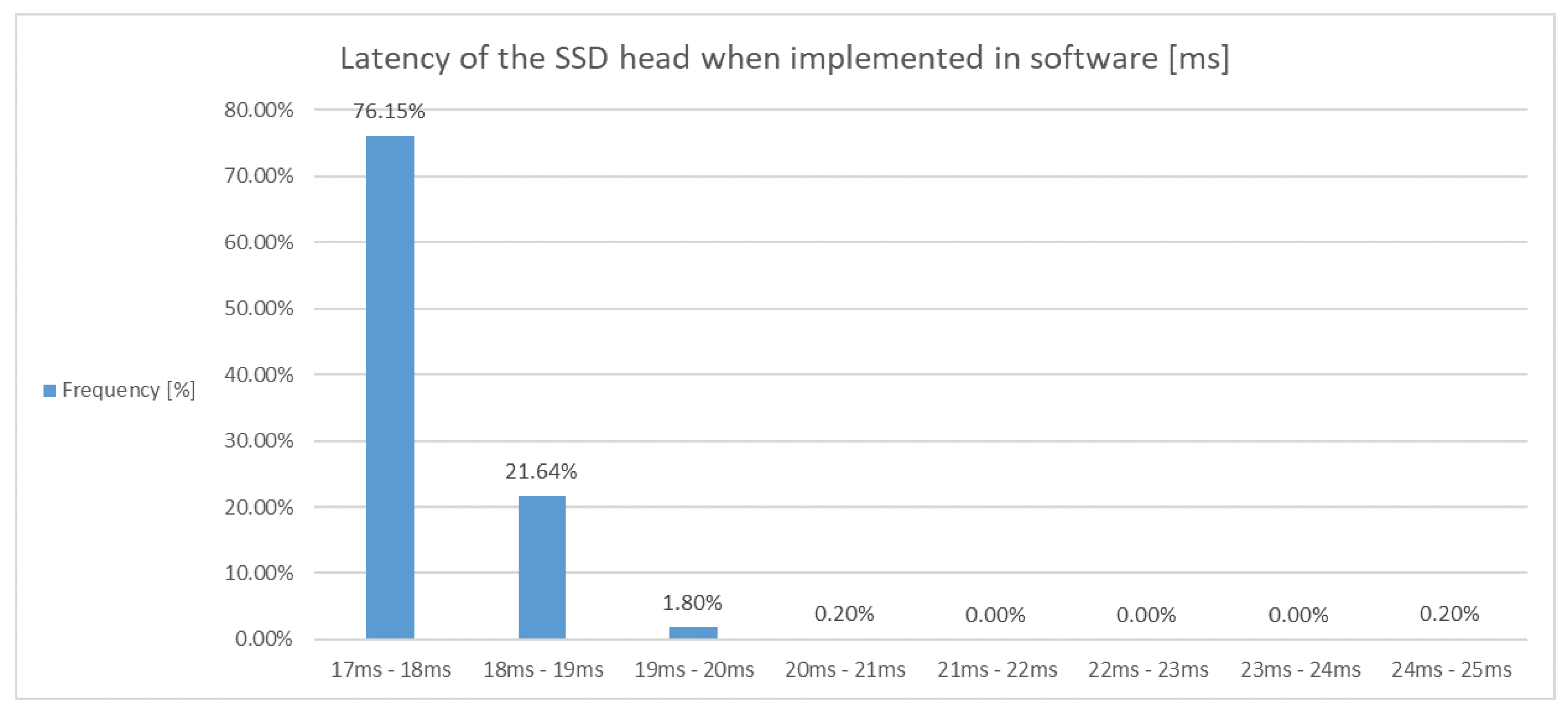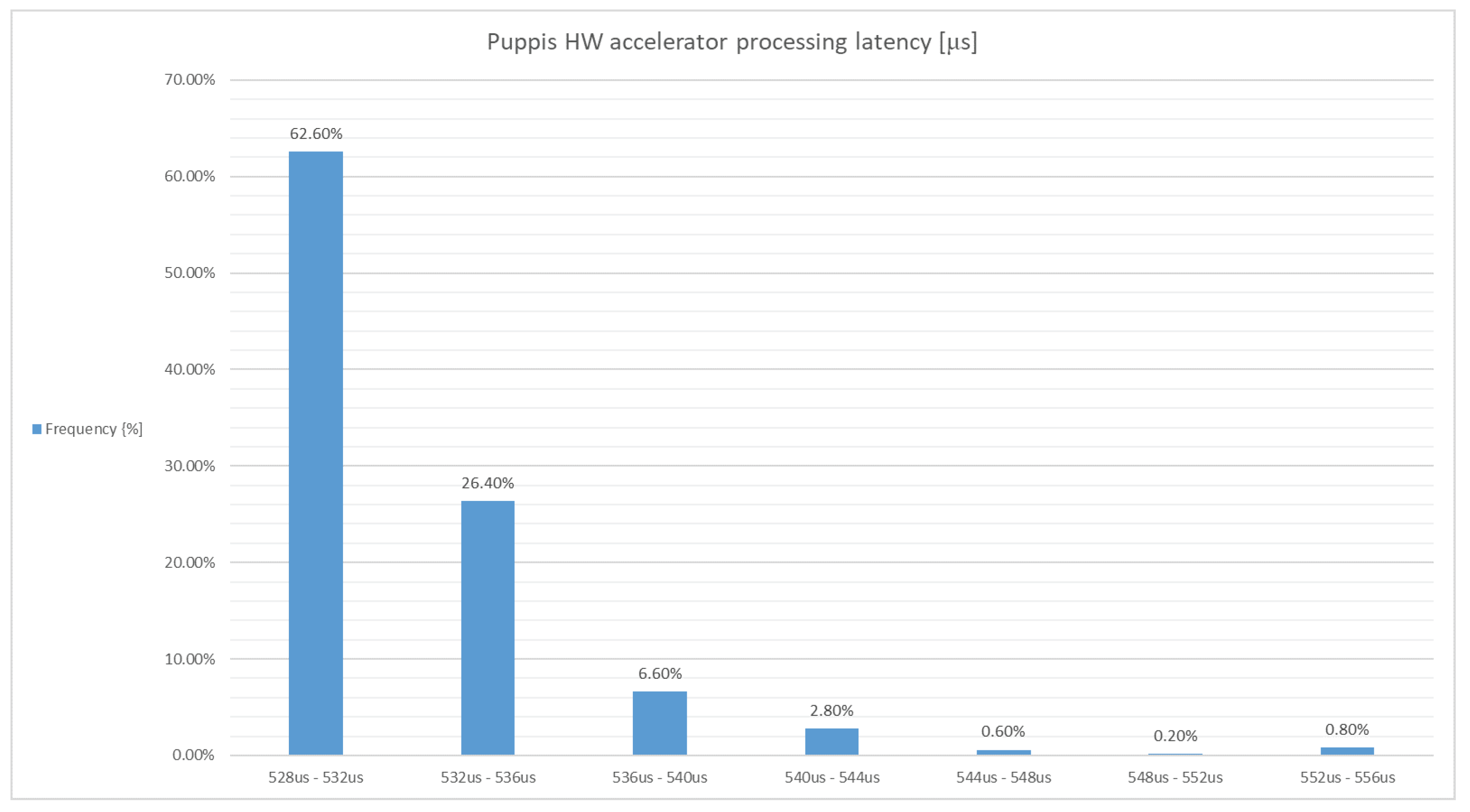As shown in [2], the SSD architecture is significantly faster than multi-stage object detectors, such as Faster R-CNN [3], while having significantly better accuracy compared to other single-shot object detectors, such as Yolo [4]. Even though the SSD post-processing algorithm is not the most-complex segment of the overall object-detection network, it is very computationally demanding and can be a bottleneck with respect to the processing latency and power consumption, especially in edge applications with limited resources. Motivated by this, in this paper, we propose Puppis, an architecture for the SSD hardware accelerator, which reduces the duration of the software-implemented SSD post-processing by 97%, on average, as we show in the section presenting the experimental results.

Despite the evolution of the original object detectors [5,6,7], deep networks for detecting objects based on the SSD are still among the most-widely used, while the scientific community has proposed many improvements to the original SSD algorithm during the years that have followed, besides the proposals for SSD algorithm speedup through GPU acceleration, as in [8]. The authors in [9] proposed a slightly slower, but more-accurate object detector based on an enhanced SSD with a feature fusion module, while the authors in [10] additionally optimized their SSD-based network for small object detection. In [11], the classification accuracy of the SSD architecture was improved by the introduction of an Inception block, which replaced the extra layers in the original SSD approach, as well as an improved non-maximum suppression method. An attention single-shot multibox detector was proposed in [12], where irrelevant information within the feature maps was suppressed in favor of the useful feature map regions. There are also multiple real-time system proposals based on the single-shot multibox detector algorithm, where either modified convolutional layers are used, as in [13], a complete backbone CNN is simplified, as in [14], or a multistage bidirectional feature fusion network based on the single-shot multibox detector is used for object detection, as in [15].

While there are numerous proposals for algorithmic improvements of the original SSD algorithm available, despite existing proposals for the hardware acceleration of other object detection architectures [16,17,18,19], there are not many proposals for the hardware acceleration of a single-shot multibox detector algorithm in the available literature. The authors are aware of only two previously published papers [20,21], who presented the acceleration of the convolutional blocks within the SSD network, without focusing on the SSD post-processing part of the network. In this paper, we propose a system for the hardware acceleration of a complete single-shot multibox detector algorithm and show how it can be integrated with a slightly modified backbone classifier (MobileNetV1) to obtain a fast and accurate object detector architecture, when implemented in an FPGA. When using hardware accelerators for the implementation of the backbone CNN in low-end, low-frame-rate applications, SSD post-processing implemented in software is acceptable since the introduced latency is significantly shorter than the latency of the backbone CNN processing. Hence, it can be either neglected or even hidden by pipelining to increase the throughput, even though the latency remains the same. Our work was motivated by the fact that SSD post-processing becomes a bottleneck for high-end applications where high frame rates are required. The results from the experimental section will show how our proposal resulted in an average SSD post-processing speedup greater than 33-times and an average complete CNN network processing speedup greater than 36-times, compared with the pure software implementation, when the MobileNetV1 SSD network was used for object detection. The rest of the paper is structured as follows: After the introductory section, in Section 2, we elaborate on the general structure of the SSD network and the purpose of accelerating the SSD post-processing algorithm. In Section 3, we show which algorithms from the SSD post-processing step are accelerated and how, while the accelerator architecture is presented in Section 4. The experimental results are shown in Section 5, while the conclusion is given in the last section.

2. Overview of Proposed System for Hardware Accelerator of Complete SSD Network

2.1. General Structure of SSD Network

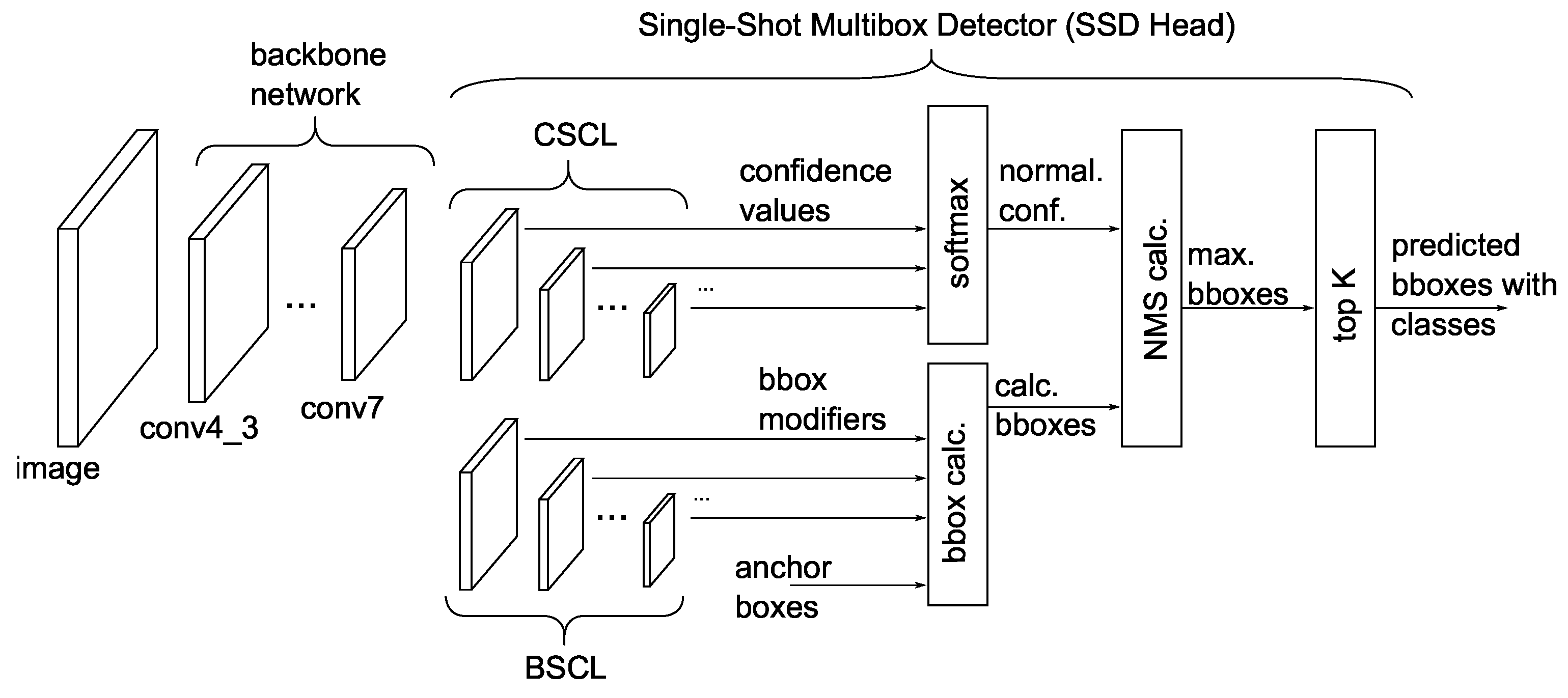
Figure 1 shows the general structure of the SSD network. The backbone network is the first component of the SSD network and employs a standard CNN such as VGG, MobileNet, ResNet, Inception, or EfficientNet. The backbone network’s objective is to extract features from the input image automatically, enabling the system to identify bounding boxes accurately.

The second part of the SSD network is the single-shot multibox detector, the SSD Head for short. The purpose of the SSD Head is to calculate the bounding boxes for every class from the results computed by the backbone part of the network. The SSD Head consists of additional convolutional layers and four other functions: softmax calculation, bounding box calculation, the Non-Maximum Suppression (NMS) function, and top-K sorting.

In the SSD Head, there are always paired convolutional layers. One layer determines the confidence values, marked as the Confidence SSD Convolutional Layer (CSCL), while the other calculates the bounding box modifiers, referred to as the Bounding Box SSD Convolutional Layer (BSCL). Additionally, there is a third layer that calculates the anchor boxes. These boxes are trainable parameters of the network, but they remain constant for every SSD network once trained.

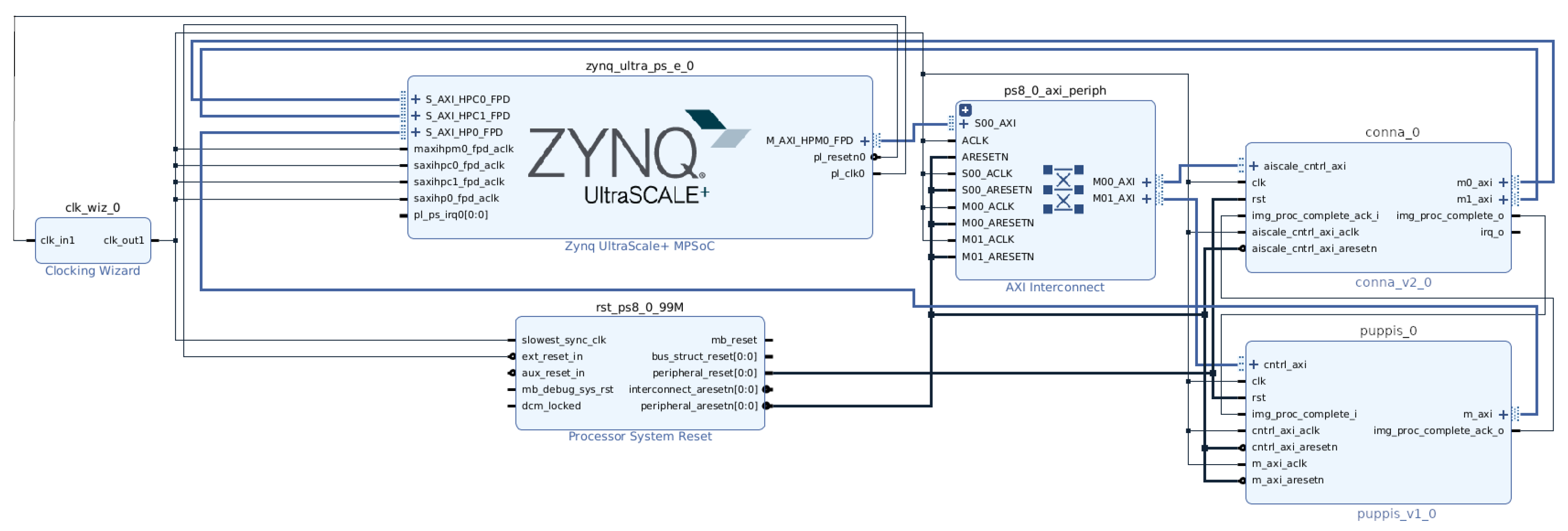
2.2. System for HW Acceleration of Complete SSD Architecture

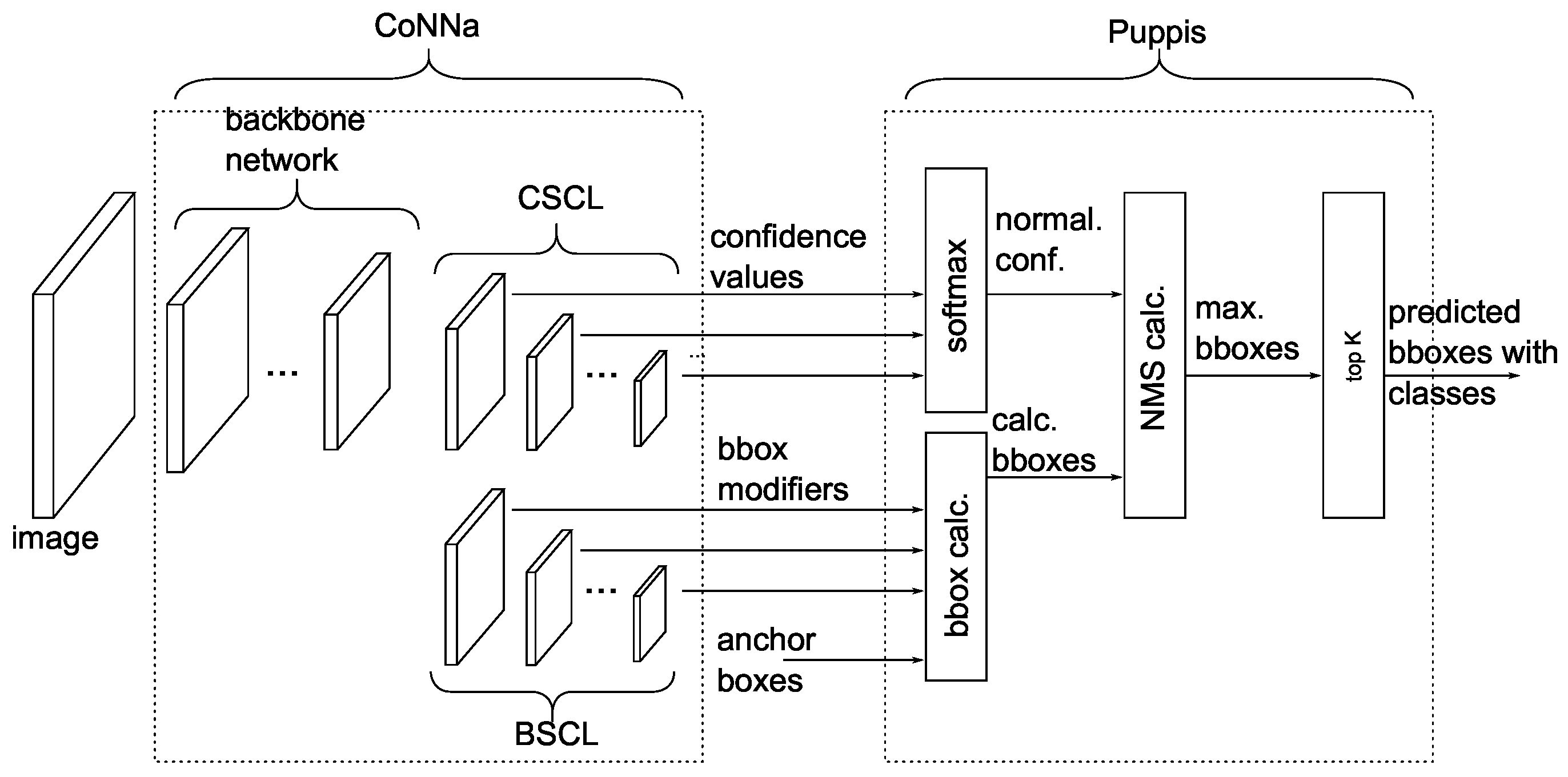
The overall system for the hardware acceleration of the complete SSD network, including Puppis, is shown in Figure 2. The Puppis accelerator must be coupled with a CNN accelerator to enable complete SSD network acceleration in hardware. The CNN accelerator will speed up both the backbone CNN network and the additional convolutional layers in the SSD Head. This paper used a modified version of the CoNNa CNN HW accelerator, proposed in [22] for this purpose. In contrast, the Puppis HW accelerator will accelerate the remaining calculating functions from the SSD Head: softmax, bounding box, non-maximum suppression, and top-K sorting. By working together, CoNNa and Puppis enable the hardware acceleration of the complete SSD network.

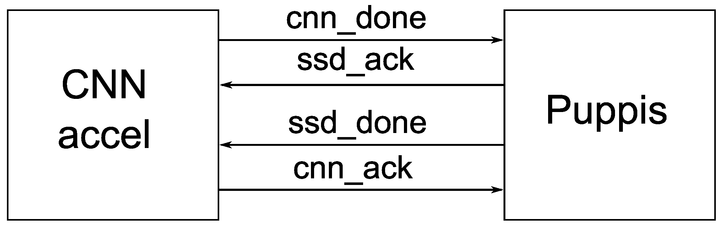
The Puppis uses two handshake interfaces, enabling an easy and generic way of connecting to the selected CNN accelerator. Please notice that, if the CNN accelerator does not already have this handshake interface, it must be adapted to support it. However, due to the simplicity of the handshake interface used, this poses no significant problem. Figure 3 shows the proposed interfaces between the two accelerators. These two interfaces will be called the SSD-CNN handshake.

Both interfaces contain only two signals. In Figure 3, the first one consists of the cnn_done and ssd_ack signals. When the CNN accelerator finishes processing the backbone network with the current input image, it asserts cnn_done. The Puppis asserts ssd_ack to acknowledge that and starts executing its part of the complete SSD algorithm using the feature maps provided by the CNN accelerator, computed using the last input image.

The second interface includes the ssd_done and cnn_ack signals. Here, Puppis asserts ssd_done when processing is complete, and cnn_ack is triggered when the CNN accelerator acknowledges it and switches to process the following input feature map.

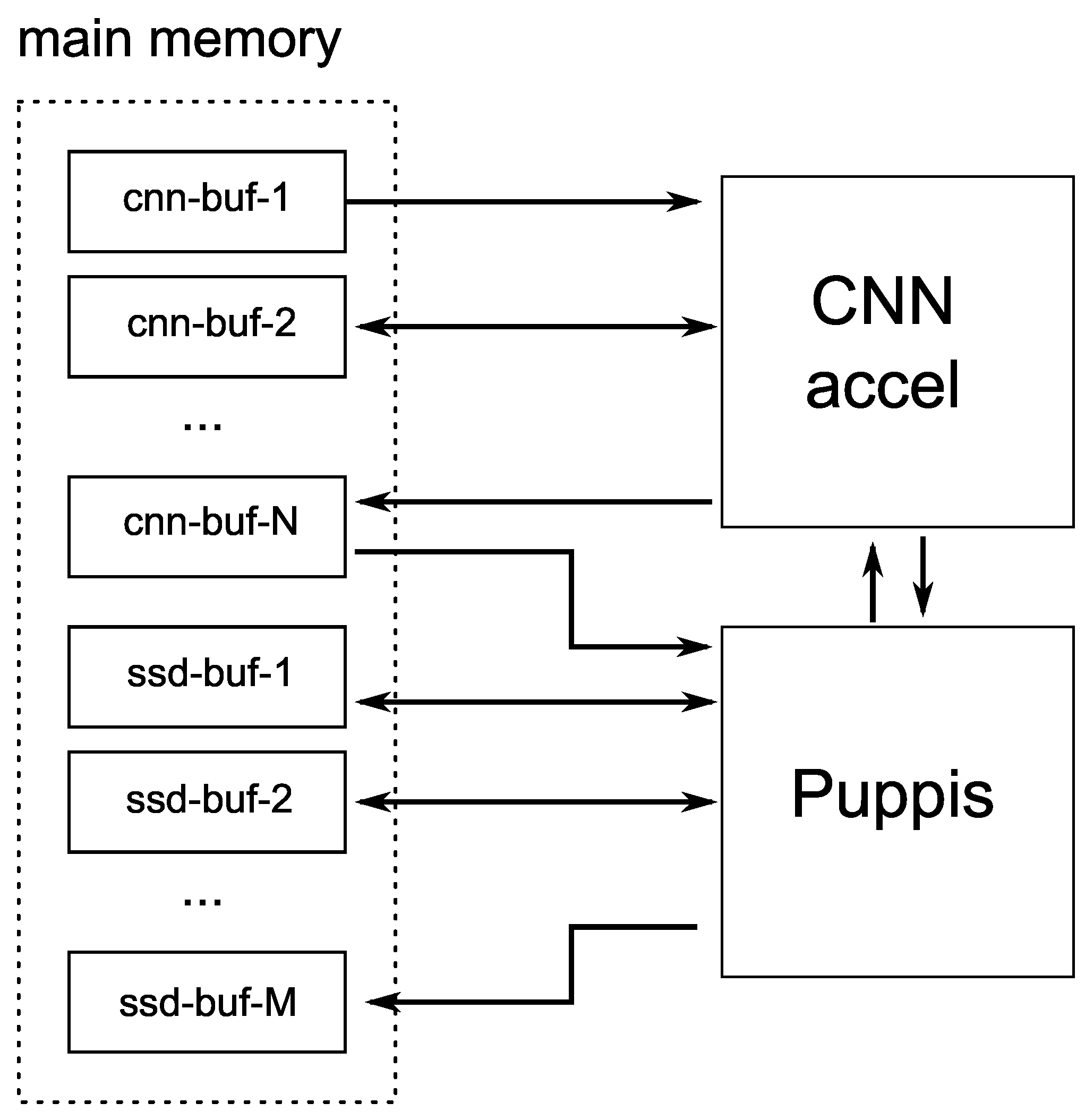
As can be seen from the previous explanation, these two interfaces enable the synchronization and reliable transfer of data between the selected CNN accelerator and Puppis SSD Head accelerator. Feature maps computed by the CNN accelerator are transferred to the Puppis using a shared memory buffer. The information presented in Figure 4 demonstrates using buffer cnn-buf-1 as the input buffer for the SSD network’s image processing. After processing the first layer, the buffer cnn-buf-2 stores the result. That buffer is then input for the next layer, and so on.

The results of processing the final layers from the CSCL and BSCL are stored in couple of last cnn-buf buffers, depending on the number of these final layers. For example, if there are k final layers, then cnn-buf-N-k up to cnn-buf-N buffers would be used to store their output values. These buffers are actually the input buffers for the Puppis HW accelerator. During its operation, Puppis uses additional memory buffers: ssd-buf-1 up to ssd-buf-M. These buffers are used to store intermediate results, computed as the Puppis HW accelerator operates on the input data. The final results are stored in the output buffer ssd-buf-M. From this buffer, the software can read the final results of the SSD network processing, containing the detected objects’ bounding box information.

Please notice that the described setup enables the implementation of a coarse-grained pipelining technique during the processing of a complete SSD network by the proposed system. While the Puppis HW accelerator processes CNN-generated information for the input image i, the CNN HW accelerator can already start processing input image i+1. This setup can significantly increase the processing throughput of the complete system, although the processing latency will remain unchanged. In applications where achieving a high frame rate is of interest, this could prove highly beneficial.

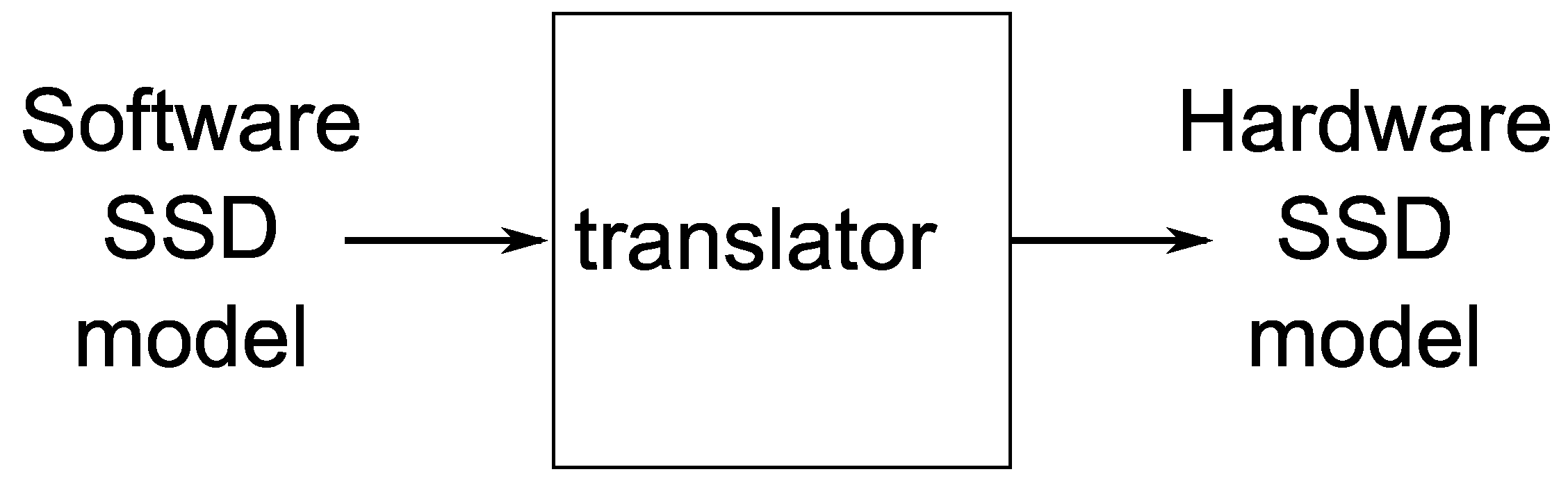
In order to be able to process the selected SSD network, both the CNN and Puppis HW accelerators require that the SSD network be represented in an accelerator-specific binary format, as shown in Figure 5. During the development of Puppis, such a tool for translating the high-level model of the SSD network (developed, for example, using Keras, PyTorch, or some other framework) into this accelerator-specific binary model was also developed.

In the process of SSD model translation, the translator tool also determines the optimal fixed-point number format that will be used to store various SSD-model-related data during the SSD network processing. Then, it translates the model parameters to this number format and stores them in buffers, which are located in the main memory of the SSD accelerator. For the anchor boxes, it prepares special buffers for Puppis, so that it can just load those values from the memory system, without any calculation. In short, this tool prepares the model to be successfully processed by the CoNNa and Puppis accelerators.

3. Accelerated SSD Head Computation Algorithms

The part of the single-shot multibox detector algorithm that is implemented by the Puppis HW accelerator contains four main computational steps:

• Softmax calculation;
• Bounding box calculation;
• NMS calculation;
• Top-K sorting.

The first three steps are more computationally complex, and the following sections contain detailed descriptions. The last part of the calculation, top-K sorting, determines the best K bounding boxes within the results calculated in the non-maximum suppression block using a simple bubble-sort algorithm.

3.1. The Softmax Calculation

The softmax calculation is the first step executed by the Puppis accelerator. The inputs for the softmax calculation are the confidence values of the SSD convolutional layers and Exponential Confidence Look-Up Tables (ECLUTs), while the outputs are the score predictions for all boxes. The confidence values are the outputs from the backbone network and the CSCL, and in our setup of the complete SSD network hardware accelerator, the modified CoNNa CNN accelerator will provide these as its output. The ECLUT is an array of samples of exponential functions in the floating-point format, which is calculated by the translator and stored in the main memory.

Equation (1) represents the softmax formula, which determines the normalized values.

$$n_k=\frac{e^{S_k}}{{\sum }_{i=1}^{i=N}{e}^{S_i}}$$

(1)

Subscript k is an index of the current class ($k\in \{1,...,N\}$); S is the input from the confidence layers; N is the number of classes; $n_k$ are the normalized confidence scores.

The hardware accelerator implementation mainly uses two number formats: fixed-point or floating-point. The simpler or energy-efficient hardware accelerators use the fixed-point format, while applications requiring a wide dynamic range utilize the floating-point format. We used a hybrid approach in this architecture, which a later section will describe. Softmax calculation uses an exponential function over a wide range of values. Therefore, if the architecture uses only the fixed-point format, it will require many bits to cover the number range. Using only the floating-point hardware would be too expensive because the floating-point calculation uses too many hardware resources. Therefore, the optimal solution requires a mix of floating-point and fixed-point numbers. In that way, we keep the hardware utilization close to the fixed-point representation and still cover the required range of values, as if the solution uses the floating-point number representation.

Inside the calculation logic, there are hardware blocks that determine the format used for representing the fixed-point numbers. The pseudocode of the algorithm for the calculation of Equation (1), with some hardware-related details, is shown below.

The parameter SCN is the current number of SSD convolutional layer pairs that the network uses and is a configurable runtime parameter. The variable confs is an input array that contains the confidence values. The confs array is stored in the main memory of the system, while the variable box_cnt counts all boxes requiring the score prediction values.

The algorithm iterates through the output feature maps generated by each CSCL shown in Figure 1. For each output point of any CSCL and for all boxes corresponding to that layer, the list of confidence values for each class (conf_box = conf[i][j][k]) is read from memory. The algorithm also reads the corresponding floating-point value from the ECLUT memory and calculates the maximum value. The comparison between exp_vals[cls] and exp_val_max is a floating-point comparison. According to the comparison result, the algorithm determines the fixed-point representation used later in the calculation. The ECLUT contains samples of exponential functions for each class used in the network: each class has 4096 samples within the ECLUT, while the translator creates the table that contains the required samples, which are represented as 16 bit-wide fixed-point numbers. The exp_sum_reduce variable stores the computed format. This number determines how much the values are shifted during the calculation, representing the number of bits after the fixed-point. The architecture uses the 32 bit IEEE 754 standard when interpreting the floating-point numbers.

The function getFormatFromFloat determines the format according to the value of the exp_val_max variable. The following loop in the code calculates the sum of all exponential function values, computing the value of the denominator from Equation (1), which is needed to determine the softmax score box predictions. If there is an overflow during a sum calculation, the fixed-point is shifted one position to the left, exp_sum_reduce += 1, and the sum is divided by 2 to be correctly interpreted by a new fixed-point format.

Finally, the new normalized score predictions, $n_k$, are calculated for all classes. A computed denominator value divides the confidence value for every class, and a score prediction array stores the result. This array’s location is in the main system memory.

3.2. The Bounding Box Calculation

The bounding box calculation is the next step in the accelerator calculation flow. For every output point in the convolutional layer that calculates the bounding box modifiers and for every anchor box, the accelerator calculates one resulting bounding box. The following formulas express the bounding box calculation procedure.

$$C_{xb}=X_p{X}_v{W}_a+C_{xa}$$

(2)

$$C_{yb}=Y_p{Y}_v{H}_a+C_{ya}$$

(3)

$$W_b=e^{W_p{W}_v}{H}_a$$

(4)

$$H_b=e^{H_p{H}_v}{W}_a$$

(5)

$$X_{min}=C_{xb}-W_b$$

(6)

$$X_{max}=C_{xb}+W_b$$

(7)

$$Y_{min}=C_{yb}-H_b$$

(8)

$$Y_{max}=C_{yb}+H_b$$

(9)

$C_{xb}$ and $C_{yb}$ are the predicted center of the bounding box. $X_p$, $Y_p$, $W_p$, and $H_p$ are four predicted input values from the convolutional layers. $X_v$ and $Y_v$ are the so-called variance values, which are trainable parameters of the SSD network, stored within a binary description of a network by the translator. The values $W_a$ and $H_a$ are the width and heights of the current anchor box, and the values $C_{xa}$ and $C_{ya}$ specify the center of the current anchor box. The values $W_b$ and $H_b$ are the output values of the convolutional layer used to calculate the width and height of the bounding box. The values $W_v$ and $W_v$ are the variance values determined during the training. Finally, the values $X_{min}$ and $Y_{min}$ specify the upper left corner of the predicted bounding box, while ($X_{max}$, $Y_{max}$) specify the lower right corner of the computed bounding box.

Puppis uses the 16 bit fixed-point number representation for all calculations (2)–(9), while the translator determines the exact position of the decimal point. Opposite the calculation of an exponential function as a part of a softmax calculation, the exponential functions in Equations (4) and (5) are calculated using look-up tables.

3.3. Non-Maximum Suppression Calculation

Once the bounding box calculation is complete, the third step is to perform the NMS calculation. This is an important algorithm that helps to remove overlapping boxes that have been placed around the same object with high confidence. The goal is to have only one bounding box around one object, so the NMS calculation removes any boxes that overlap enough (the algorithm parameter). This step ensures that there is only one bounding box around each object, even if there were originally several boxes before this step.

The pseudo-code for this algorithm is listed below. The inputs for this algorithm are the confidence values after the softmax calculation, calculated in Step 1, and the bounding box locations calculated in the second step. These inputs are represented as the in_confs variable for the confidences and in_bboxes for the bounding boxes. confs is a 2D array because it holds the normalized confidence values for all the classes and all the bounding boxes.

The algorithm iterates over all classes, where the variable cnt_class represents the current class. The variable box_ind represents the indices of the confidence values more significant than the input threshold TVAL. The variable confs is all the confidence values greater than TVAL, and the variable bboxes is the corresponding bounding boxes. If no such values exist, the algorithm iterates to the next class. The variable areas represents areas of all bboxes, while the variable sort_ind is a sorted version of box_ind, and the indices are sorted based on their corresponding confidence values. The value gt_ind represents the index of the bounding box with the maximum confidence value for the current class. The outputs of the algorithm are the bounding boxes for which the confidence value is greater than a user-defined parameter TOVER. Each of these bounding boxes is accompanied with its class membership information. The algorithm calculates the overlap between the current best bounding box and all other bounding boxes, so the subsequent while loop iteration only processes indices with overlaps less than a threshold value of TOVER. The while loop terminates if no such indices exist (the sort_ind list is empty), and the algorithm outputs all possible bounding boxes for each class with a confidence value above the TVAL parameter, for which it holds that the overlap with the best confidence box that is lower than TOVER.

Function calc_overlap calculates the overlap between two boxes, after receiving two rectangles as inputs. The first rectangle is defined by two points, $(X_{min1},Y_{min1})$ and $(X_{max1},Y_{max1})$, and the second by $(X_{min2},Y_{min2})$ and $(X_{max2},Y_{max2})$. The function calculates the overlap value according to the following formulas:

$$X_{min}=max(X_{min1},X_{min2})$$

(10)

$$Y_{min}=max(Y_{min1},Y_{min2})$$

(11)

$$X_{max}=min(X_{max1},X_{max2})$$

(12)

$$Y_{max}=min(Y_{max1},Y_{max2})$$

(13)

$$A_i=(X_{max}-X_{min})(Y_{max}-Y_{min})$$

(14)

$$A_u=A_1+A_2-A_i$$

(15)

$$O=\frac{A_i}{A_u}$$

(16)

where the points $(X_{min},Y_{min})$ and $(X_{max},Y_{max})$ define an overlapping rectangle. The overlapping area is $A_i$; $A_u$ is a non-overlapping area, while the values $A_1$ and $A_2$ represent the areas of the two bounding boxes, for which the calculation is performed. The value $A_1$ is always the area of the bounding box with the greatest confidence value for the current class, while the output of the function O represents a ratio between $A_i$ and $A_u$.

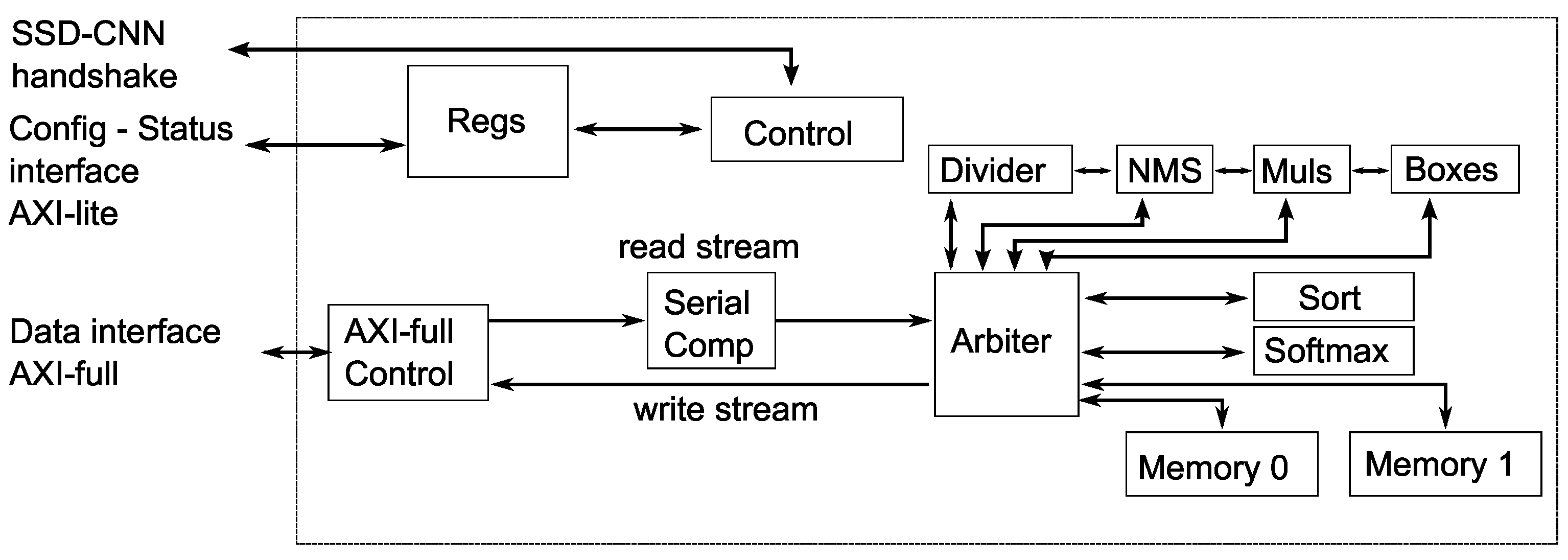
4. Puppis HW Accelerator Architecture

Figure 6 provides an overview of the architecture of the Puppis hardware accelerator. It shows the interfaces and central building blocks at the highest abstraction level. Puppis uses three interfaces to connect to surrounding modules: the configuration and status AXI-Lite interface, the data transfer AXI-Full interface, and the SSD-CNN handshake explained earlier in Section 2.2.

The AXI-Lite interface configures and checks the accelerator status, while the AXI-Full interface transfers data to and from the accelerator. The Arbiter module is responsible for routing data throughout the accelerator. Additionally, the SSD-CNN handshake interface enables the calculation of the entire SSD CNN without needing processor intervention.

At the top level, Puppis has multiple modules. Among them is the Regs module, which comprises the accelerator’s configuration registers. Additionally, Puppis has status registers accessible through the AXI-Lite interface. The configuration settings impact the functionality of the central controller module, represented as Control in Figure 6.

The Control module coordinates the other modules’ operations to calculate the SSD Head output. Depending on the configuration and calculation state, this module controls the routing and timing of data transfers through the accelerator’s calculation modules and their internal pipeline stages. Although it has connections to all other modules, Figure 6 does not show these connections for clarity. The following section will provide a more-detailed description of this module.

The Arbiter module serves as the primary data-routing unit in Puppis. Its interconnect architecture allows for seamless data transfer from its source to its destination, making it an integral part of the Puppis accelerator. The main Control module is responsible for controlling the Arbiter module’s operations.

The main calculation modules of Puppis are Softmax, Boxes, and NMS. The Softmax module calculates the softmax function, given by Equation (1) and Listing 1. The Boxes module calculates the bounding boxes, Equations (2)–(9). The NMS module calculates the NMS function of the SSD calculation; see Listing 2. The following sections will describe these modules in more detail.

Listing 1. Softmax pseudocode.

box_cnt = 0

for ci in (0 to SCN):

conf = confs [ ci ]

for i in (0 to Heights [ ci ]):

for j in (0 to Widths [ ci ]):

for k in (0 to Box [ ci ]):

conf_box = conf [ i ][ j ][ k ]

exp_val_max = 0

for cls in (0 to ClassN):

exp_in_val = conf_box[cls] >> 4

exp_vals[cls] = ECLUT[ci][exp_in_val]

if (exp_vals[cls] > exp_val_max):

exp_val_max = exp_vals[cls]

exp_fmt = getFormatFromFloat(exp_val_max)

exp_sum = 0

exp_sum_reduce = 0

for cls in (0 to ClassN):

exp_vals_sum[cls] =

floatToFixedConv(exp_vals[cls], exp_fmt)

exp_sum += exp_vals_sum[cls]

if (overflow(exp_sum)):

exp_sum /= 2

exp_sum_reduce += 1

for cls in (0 to ClassN):

exp_val = exp_vals_sum[cls] >> exp_sum_reduce

scores_predictions[cls][box_cnt] = exp_val / exp_sum

box_cnt += 1

Listing 2. NMS pseudocode.

for_each cnt _ class in classes

box_cnt += 1for_each cnt_class in classes

box_ind = indices_greater_than_value(cnt_cls, in_confs, TVAL)

confs = values_from_indices(in_confs, box_ind)

bboxes = values_from_indices(in_bboxes, box_ind)

if confs empty go to next class

for_each box in bboxes

areas = area_of(box)

sort_ind = sort_indices_by_conf( box_ind, confs )

while sort_int not empty

gt_ind = sort_ind[0]

resutls_add(bboxed[gt_ind], cnt_class, confs[gt_ind])

for_each ind in sort_ind except gt_ind

put calc_ovelap(bboxed[gt_ind], bboxed[ind]) into overs

sort_ind = get_indices_for_which_overlap_less_than(

sort_ind, overs, TOVER)

The other helper calculation modules of Puppis are: Divider, Muls, and Sort. Specifically, the Divider module implements the division operation of two fixed-point numbers, used in the Softmax and NMS computational steps of the SSD algorithm. It uses a pipelined architecture to achieve a similar operating frequency as the other modules. The Muls module calculates the multiplication of two fixed-point numbers represented with the same number of bits. This module is pipelined and has four lanes to calculate four multiplications simultaneously. The Sort module sorts values and is used during the NMS calculation and for selecting the final top K results.

Puppis uses two internal caching memories: Memories 0 and 1. They store the configuration parameters and intermediate results during the SSD calculation. The memories are configurable and have several purposes during the SSD calculation process, which the following sections will describe in more detail.

The Arbiter module enables communication between the calculation modules and the memories. Additionally, some communication lines connect the calculation modules directly: Divider to NMS, NMS to Muls, and finally, Muls to Boxes. These lines stream intermediate results, without buffering, between modules.

An AXI-Full interface enables communication to the external main memory. The AXI-Full Control module implements the AXI-Full protocol. This module receives two AXI-Stream data streams, a read stream and a write stream, and combines them into a single AXI-Full interface.

The Serial Comp module connects to the Arbiter and the AXI-Full Control module’s read interface. The module reads the confidence predictions from the main memory and passes only those predictions greater than the predefined threshold to the Arbiter module. Furthermore, the Serial Comp module can transfer other data types without discrimination.

The forthcoming sections will concisely explain the most-essential modules’ operational principles. The descriptions will omit specific details to offer a broad overview of each modules’ functioning and facilitate comprehension.

4.1. Control Module

The Control module sends control signals to all the other modules in the architecture. It implements a Finite-State Machine (FSM), which sequentially processes the input through several steps of the SSD Head computation algorithm explained earlier. Figure 7 shows the simplified FSM.

In the READY state, Puppis is ready to receive the subsequent input. In this state, the module AXI-Lite can change configuration to prepare calculation blocks to process the input. In the next state, Softmax, the Control module sends control signals to read the input confidence values from memory, calculate the softmax algorithm with those inputs, and write the normalized values into the main memory. In the Boxes state, Puppis reads the bounding box modifiers from the main memory and anchor boxes, then calculates the bounding boxes. Internal memory modules store the resulting bounding boxes. In the NMS state, the Control unit sends control signals to receive the normalized confidence values from the main memory and the bounding boxes from the internal memory. Then, the NMS algorithm processes those inputs, and the internal memory stores the resulting output. Finally, in the Sort state, the inputs from the NMS step are read from the internal memory, and the best calculated K results are stored in the main memory as the final result of the input processing. Then, the Puppis accelerator switches to the READY state, being ready to receive the next input.

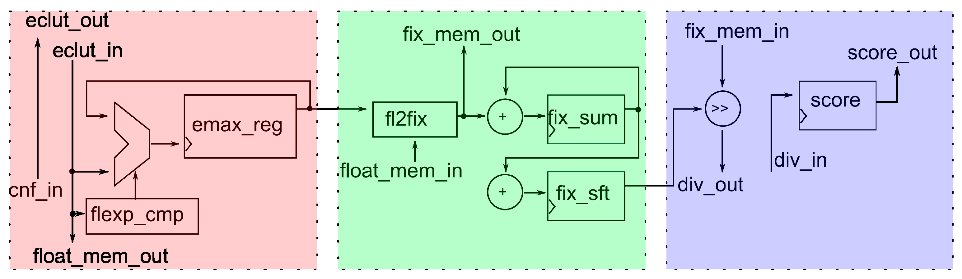
4.2. Softmax Module

Figure 8 shows the top-level block diagram of the Softmax module. The block diagram presents a model of the Softmax module close to the Register Transfer Level (RTL), but some details are abstracted. In this way, the model is easier to explain. For example, the model does not show the control signals from the Control module. We call this model the abstracted RTL model. The Softmax module contains three pipeline stages.

The module receives confidence values from the main memory in the first pipeline processing stage. The module determines the maximum value of the floating-point exponent by utilizing samples of a floating-point function stored in the ECLUT memory. This value is stored in the output register flexp_cmp and serves as the input for the second pipeline stage.

Based on the format determined in the first phase, the module converts all floating-point values $e^{S_k}$ from the Formula (1) into the fixed-point format in the second phase of the pipeline processing. The internal memory receives the numbers in the new number format through the fix_mem_out port. Additionally, this module computes the sum from the Formula (1). If overflow occurs, the module adjusts the number format accordingly.

The module divides the fixed-point values $e^{S_k}$ in the third phase by the computed sum. During this calculation, the module utilizes the Divider module. The final result, representing normalized values from the Formula (1), is stored in internal memory with the score_out port, making it available for other modules for further processing.

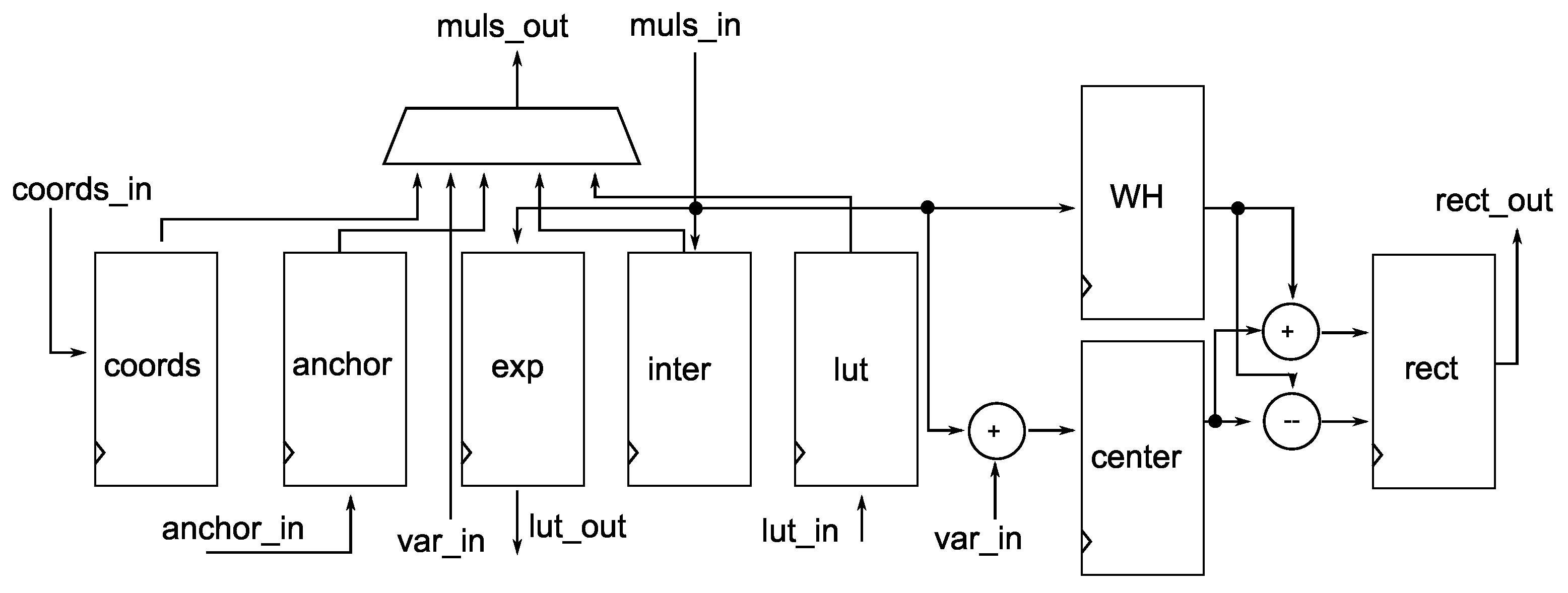
4.3. Bounding Box Module

Figure 9 shows the abstracted RTL model for the Bounding box module. The module uses several registers to store intermediate calculation results for Equations (2)–(9). The top of Figure 9 shows the multiplexer, which the Control module uses to select which arguments to send to the Muls module.

This module encompasses numerous registers designed to store intermediate computation results. Over several clock cycles, the center coordinates of the bounding box are computed and stored in the center register, while the register, denoted as WH, holds the calculated width and height values. The module computes the resulting rectangle, utilizing these center coordinates and dimensions, and forwards it to the internal memories through the port rect_out, making it available for other modules.

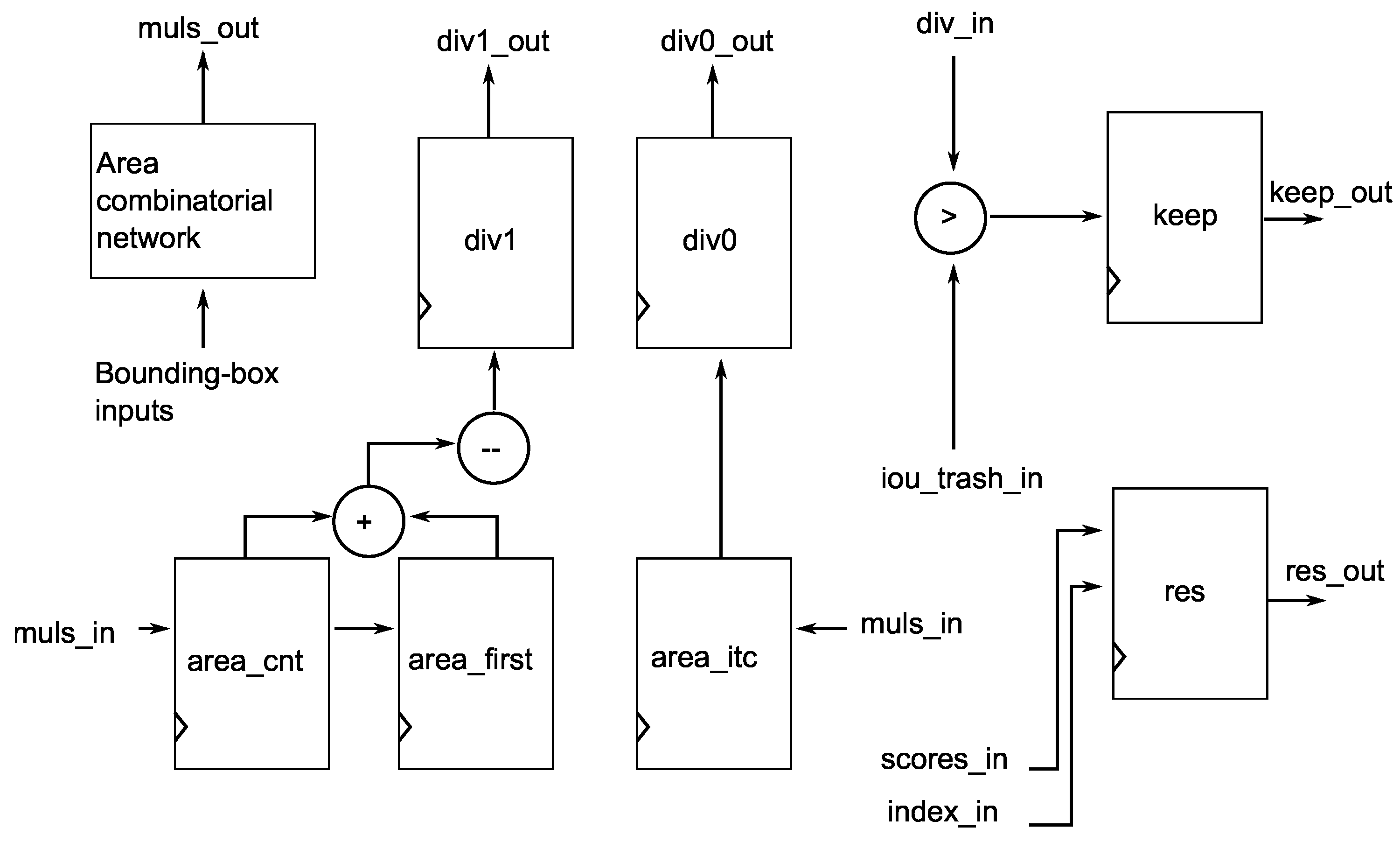
4.4. NMS Module

The Control module guides the NMS module through Listing 2. The core of that algorithm is Equations (10)–(16). Figure 10 shows an abstract RTL schematic of the NMS module. The following is a description of how the module calculates these equations.

In the initial step, this module calculates the areas of the bounding boxes based on the results computed by the Bounding box module. During its operation, for all multiplication operations, this module utilizes the Muls block. For all boxes, except the first one, the module calculates O from Equation (16). The Divider block is employed when division is required, and the module obtains the O value through the dib_in port. Subsequently, O is compared to a threshold parameter to determine whether the module retains the bounding box. The keep register holds this information. Along with this information, the module sends the confidence and computed bounding box values (res register) needed for final result sorting.

4.5. Sort Module

The computation’s last step is the top-K sorting procedure, which identifies the top-K bounding boxes from the results obtained through the non-maximum suppression block. The implemented sorting procedure is a simple bubble-sort algorithm. Since this step does not require much computation, a simple sequential architecture is used for this module.

5. Experimental Results

To assess the performance of Puppis and compare it with the MobileNetV1 SSD network’s software implementation, we conducted experiments on the Zynq Ultrascale+ MPSoC ZCU102 Evaluation Board [23]. The timings presented in this section are the measured results obtained from the experimental setup, not simulated values. As was already stated in the Introduction, to the best of the authors’ knowledge, there are no previously proposed solutions for the HW acceleration of the SSD Head part of the SSD network. Therefore, a direct comparison of Puppis with previously proposed HW accelerators was not possible.

5.1. Hardware Setup

In order to assess the effectiveness of the proposed architecture, we utilized an FPGA development platform to implement the entire SSD network hardware acceleration system, presented in Figure 2. For the design and implementation, we relied on the Xilinx Vivado Design Suite [24]. The hardware platform we used for conducting the experiments was the Zynq Ultrascale+ MPSoC ZCU102 Evaluation Board [23]. We utilized the default synthesis and implementation settings in the implementation tools during the implementation. Figure 11 displays the Vivado IP Integrator top-level block diagram of the system we developed for the experiments.

The central parts of the system are Zynq’s processing system and the CoNNa and Puppis HW accelerators. After the implementation, the achieved maximum operating frequency of the complete system was 180 MHz. The resource utilization is shown in

Table 1. FPGA implementation results.

Component	LUT	BRAM	DSP
Puppis	4055	17.5	4
System	103766	326.5	446

.

As can be seen from Table 1, the Puppis accelerator uses only a fraction of the consumed hardware resources required to implement a complete SSD network accelerating system. It uses a mix of all FPGA resources, which is a desirable feature. Compared to the whole system, the utilization of LUTs was 3.91%, BRAM was 5.36%, and DSP was below 1%. The CoNNa accelerator uses most hardware resources. Puppis’s hardware consumption will be negligible even if another CNN accelerator is used instead of CoNNa. Incorporating the Puppis SSD Head HW accelerator will not significantly increase the overall HW resource consumption, which could otherwise hinder the successful implementation of the system for most existing AI systems that already use hardware CNN acceleration. However, as the next section will demonstrate, including the Puppis HW accelerator in the system can significantly enhance the processing speed of SSD networks.

Table 2. Power consumption.

Component	Absolute Power (W)	Power Percentage
System	5.919	100
Zynq PS	2.757	46.579
CoNNa	2.964	50.076
Puppis	0.088	1.487

presents Vivado’s power consumption estimation for the entire SSD acceleration system. As can be observed, the Puppis accelerator consumed 0.088 W, constituting only 1.487% of the system’s total power consumption. The CNN accelerator accounted for 50.076% of the power consumption, while the system’s processor consumed a similar amount of power, accounting for 46.579%. Based on these numbers, it is reasonable to conclude that the power consumption of the Puppis accelerator is negligible compared to the rest of the system. However, the speed improvement is significant, as demonstrated in the subsequent section.

5.2. Software Comparison

In order to evaluate Puppis, a comparison with software SSD network processing was performed. Additionally, to obtain relevant results, the software was run on the Ultrascale+ MPSoC ZCU102 evaluation board [23] running the Ubuntu 20.04 Operating System. The SSD network chosen for the comparison was the MobileNetV1 SSD network, trained on the Pascal VOC dataset [25]. The MobileNetV1 SSD network model was built using the Tensorflow framework [26], but split into the backbone CNN part, accelerated by the CoNNa CNN accelerator, and the part of the network that will be run using the Puppis accelerator. This split was performed to accurately evaluate the performance of each submodule. During the evaluation, images from the Pascal VOC dataset were used, both for the inference in the software and hardware accelerator.

At the beginning, the goal was to prove that the hardware acceleration of the SSD Head will not reduce the accuracy of the software model.

Table 3. mAP calculated on the images from the Pascal VOC dataset.

Dataset	mAP SSD Head SW	mAP Puppis
Pascal VOC 2007	62.28%	61.9%

shows that the performance of an object detector was not degraded after quantization and migration to a fixed-point number representation. The accuracy of the software implementation and the Puppis HW accelerator, presented in the table, is expressed in terms of the mean Average Precision (mAP), a standard object-detection metric. From Table 3, it can be seen that switching from the software implementation of the SSD Head based on a floating-point number representation to the Puppis HW accelerator, which uses fixed-point number arithmetics, led only to a minor mAP drop, less than 0.3% in the absolute value.

In order to explore the impact of different test instances on the processing latency, images from the Pascal VOC dataset [25] were used for the processing latency histograms shown in Figure 12 and Figure 13.

Figure 12 shows that, when executing the SSD Head in the software, the latency duration for more than 99% of the test instances ranged from 17 ms to 20 ms. Similarly, from Figure 13, around 90% of the test instances resulted in a latency duration between 528 and 536 µs, when the SSD Head ran on the Puppis HW accelerator. On rare occasions, the input images have a significantly larger number of objects within the image, which led to a slightly longer processing latency: up to 25 ms for the software implementation and up to 556 µs for the SSD Head running on the Puppis HW accelerator.

The processing latencies while detecting objects in the image using hardware accelerators CoNNa and Puppis are shown in the table below.

As can be seen from

Table 4. Mean value and standard deviation of the processing latency when detecting objects from the Pascal VOC [25] images by CoNNa and Puppis.

Dataset	CoNNa Latency (ms)	Puppis Latency (ms)
Pascal VOC 2007	16.61 ± 0.0054	0.5325 ± 0.0035

, the processing latencies for both CoNNa and Puppis had a minimum deviation and were executed in almost constant time, independent of the image being processed or the number of detected objects within the image. This feature represents the additional benefit of using hardware accelerators for CNN processing, since the constant processing time is highly appreciated in most applications.

Table 5. Mean value and standard deviation of the processing latency when detecting objects from the Pascal VOC [25] images by the software implementation of the MobileNetV1 SSD network.

Dataset	Backbone CNN	SSD Head
	Latency SW (ms)	Latency SW (ms)
Pascal VOC 2007	607.005 ± 67.017	17.754 ± 0.4833

presents the processing latencies for the backbone CNN network and single-shot multibox detector when both of them were executed by the embedded ARM processor, present in the Zynq MPSoC system. As in the case of the hardware measurements, the MobileNetV1 SSD network was used.

It can be seen from Table 5 that the execution of the SSD network using an embedded processor, as expected, took significantly more time, when compared to the hardware-accelerated processing of the same set of images.

Table 6. Single-shot multibox detector processing latency reduction and speedup when using the Puppis HW accelerator.

Dataset	SSD Head Latency Reduction (%)	SSD Head Speedup
Pascal VOC 2007	96.998 ± 0.079	33.34 ± 0.921

,

Table 7. MobileNetV1 SSD latency reduction and processing speedup when using both CoNNa and Puppis.

Dataset	MobileNetV1 SSD Network	MobileNetV1 SSD
	Latency Reduction (%)	Network Speedup
Pascal VOC 2007	97.234 ± 0.2127	36.45 ± 3.915

and

Table 8. MobileNetV1 SSD latency reduction and processing speedup when using Puppis instead of the SW SSD Head implementation.

Dataset	MobileNetV1 SSD Network	MobileNetV1 SSD
	Latency Reduction (%)	Network Speedup
Pascal VOC 2007	50.11 ± 0.684	2.005 ± 0.0282

show different processing latency reductions and processing speedups, calculated as:

$$latency\_reduction=(t_1-t_2)/t_1\times 100$$

(17)

$$speedup=t_1/t_2$$

(18)

First, when calculating Equations (17) and (18), we used the software-implemented SSD Head processing duration for $t_1$ (Column 3 of Table 5) and the SSD Head processing duration of Puppis for $t_2$ (Column 3 of Table 4). The Latency reduction and speedup were calculated for each image from the dataset, and Table 6 shows the mean value and the standard deviation of these per-image calculations.

The goal of our second test was to evaluate the performance improvement obtained after the complete MobileNetV1 SSD network running in software was substituted with a hardware-accelerated SSD network (comprising the CoNNa CNN accelerator and the Puppis single-shot multibox detector accelerator). Again, the latency reduction and speedup were calculated using Equations (17) and (18), for each image from the dataset, and their mean value and standard deviation are presented in Table 7. When calculating Equations (17) and (18) for each image, $t_1$ is obtained as the sum of the software implementation execution durations, both for the backbone CNN and the SSD Head (statistically represented by Columns 2 and 3 of Table 5). Similarly, $t_2$ is calculated as the sum of the CoNNa and Puppis processing durations, whose mean values and standard deviations are given in Columns 2 and 3 of Table 4).

Finally, as a result of our last test, Table 8 statistically presents the latency reduction and speedup in a setup where the backbone network processing was executed by the CoNNa hardware accelerator, while the SSD Head post-processing was executed by the SW in the first scenario and executed by Puppis in the second scenario. Hence, $t_1$ from Equations (17) and (18) is calculated as the sum of the CoNNa execution latency (Column 2 of Table 4) and the software-implemented SSD Head processing latency (Column 3 of Table 5). Similarly, for each image, $t_2$ is calculated as the sum of the CoNNa execution latency and the Puppis execution latency (Column 3 of Table 4), while the mean value and the standard deviation of the latency reductions and speedups are shown in Table 8.

From Table 6, it can be seen that using Puppis for the acceleration of the SSD Head reduced the time by 97% on average and led to an average speedup of 33.34-times, when compared with the SW implementation executed using the embedded ARM processor. Table 7 shows that the average MobileNetV1 SSD execution duration reduction was 97.234% when the hardware accelerators CoNNa and Puppis were used for running the backbone network and SSD post-processing, compared to the software implementation, while the average speedup was 36.45-times in this scenario. Finally, the performance improvement due to using Puppis to execute the SSD Head, instead of the software, can be observed from Table 8. This table shows that the average MobileNetV1 SSD network execution duration reduction was 50.11%, with an average speedup of 2-times, when Puppis was used for SSD post-processing instead of the software implementation, while the backbone network was running on CoNNa in both cases.

6. Conclusions

This paper presented Puppis, a hardware accelerator for the single-shot multibox detector, a popular network architecture for object detection. Our research was motivated by the fact that the software implementation of the single-shot multibox detector algorithm has become a bottleneck for both throughput and latency, after the backbone CNN processing latency has been shortened significantly recently, by using dedicated CNN hardware accelerators. Hence, to overcome this issue, the target for the proposed hardware accelerator was to shorten the execution of all processing blocks within the SSD Head algorithm: Softmax, Bounding box, and Non-maximum suppression calculation, as well as top-K sorting. Even though the proposed solution can be integrated with any classifier backbone CNN, during our experiments, we used the MobileNetV1 SSD network. By performing tests on images from the Pascal VOC dataset [25], the results showed that the hardware-accelerated single-shot multibox detector part of the complete SSD network reduced the SSD Head execution time by 97% on average, resulting in an average speedup of 33.34-times, when compared to the software implementation. The performance improvement was even higher when the complete MobileNetV1 SSD network was running on the CoNNa and Puppis hardware accelerators, instead of the software: the processing latency was reduced by 97.234% on average, leading to an average speedup of 36.45-times.