Business Purchase Prediction Based on XAI and LSTM Neural Networks

Abstract

The black-box nature of neural networks is an obstacle to the adoption of systems based on them, mainly due to a lack of understanding and trust by end users. Providing explanations of the model’s predictions should increase trust in the system and make peculiar decisions easier to examine. In this paper, an architecture of a machine learning time series prediction system for business purchase prediction based on neural networks and enhanced with Explainable artificial intelligence (XAI) techniques is proposed. The architecture is implemented on an example of a system for predicting the following purchases for time series using Long short-term memory (LSTM) neural networks and Shapley additive explanations (SHAP) values. The developed system was evaluated with three different LSTM neural networks for predicting the next purchase day, with the most complex network producing the best results across all metrics. Explanations generated by the XAI module are provided with the prediction results to the user to allow him to understand the system’s decisions. Another benefit of the XAI module is the possibility to experiment with different prediction models and compare input feature effects.

1. Introduction

The Industry 4.0 paradigm has the goal of automating all business processes and replacing human workers wherever that is possible. The application of technologies belonging to Industry 4.0 is an ongoing process. The introduction of artificial intelligence into business systems is part of this process. The role of AI systems is to make recommendations, classify instances of specific objects, perform predictions of future values for certain features, etc. The performance of these systems is measured with metrics appropriate for the specific task the system is performing. However, especially in domains dealing with sensitive data (medicine, military) [1,2], for the system to be used in practice, trust in the system is also required. Many AI systems, such as neural networks, operate as black boxes, i.e., the users only know the input and expected output but not how the input is transformed to produce the output [1]. It is, therefore, expected that trust in such a system is difficult to achieve. Explainable artificial intelligence (XAI) gives a means to justify and interpret the decisions made by the system and makes the process transparent to the user. Its main focus is to explain the reasoning of an AI model. When the user understands why the system has produced a specific output, they can view it critically and make a judgment about it more easily [2]. Mistakes are, therefore, easier to distinguish, but some peculiar decisions may seem more understandable and appropriate. The goal of incorporating XAI can be viewed as keeping the humas in the loop and in the center. This goal aligns with the arising Industry 5.0 paradigm, where expert workers will manage and oversee automated processes, creating collaboration between humans and machines [3]. Domain experts must be confident that the system makes appropriate decisions in order to enforce them.

There are different approaches to introducing explainability into a machine learning system. Two main directions are developing systems that already include explainability at their core and adding explainability components to existing systems [1]. Both approaches have benefits and disadvantages. While developing an innately explainable system seems like a superior proposition, it may result in a system with inferior performance, either in efficiency or accuracy [1,4]. Additionally, it may be more expensive or more complicated to design and build a new explainable system than to upgrade an existing well-performing system by incorporating an explainability module. This was the scenario considered while creating the architecture proposed in this paper.

In a business setting, prediction of future purchases and their details is needed for many different purposes, including product procurement planning, personalized advertising, and lost customer detection. For the purposes of this research, the hypothesis considered is that the problem of purchase prediction can be successfully addressed using machine learning techniques and explainable AI. This can be achieved by the development of an architecture for an explainable purchase prediction system. In this paper, an architecture for an explainable purchase prediction system will be proposed. The proposed architecture will be further implemented for a business purchase prediction setup for a medical drug company and subsequently evaluated in multiple phases.

The main novelty and contribution of the research described in this paper is the proposed architecture for an explainable purchase prediction system for application in a B2B setting. The emphasis on business is needed due to the different nature of decision-making in personal and business purchases, which is ultimately reflected in the resulting time series. Business purchasing decisions are based on factual needs and undergo a formal process, while personal purchases often satisfy a desire, which makes them more impulsive and harder to predict [5].

Additional scientific contribution lies in the implementation of the proposed architecture on an example of purchase prediction for medical drug sales transactions time series, which is titled Business Purchase Prediction based on XAI and LSTM neural networks (BPPXL). For incorporating explainability into this system, the Python SHAP library was utilized. The system is evaluated for three different input feature combinations and network structures in terms of prediction accuracy metrics and explainability.

The rest of this paper is organized into the following sections. Section 2 contains an overview of related work. Section 3 describes the proposed architecture of an explainable purchase prediction system for application in business. Section 4 contains a description of the method used for the implementation of the proposed architecture based on an example purchase prediction for medical drug sales transactions over a time series. Section 5 presents the experiments conducted and a discussion of the results. Finally, Section 6 consists of conclusions and possible directions for future work.

2. Related Work

2.1. Explainable Artificial Intelligence

Most of the existing literature on XAI deals with the problem of classification, specifically assigning a single class to an instance described by selected input features [6]. Another common theme is that most researchers focus on image and text classification, presumably because features derived from images and text can be more understandable to humans than numerical features. However, there are some research studies geared towards explainability in systems that solve regression problems. Conclusions that can be derived from these research studies are that not all XAI methods are suitable for regression and that applying them to regression is not always straightforward. Additionally, the authors of [6] explicitly recommend SHAP as one of the preferred methods to use when dealing with a regression problem. Perhaps this is indicative of the need to define individual approaches to XAI incorporation for different classes of problems.

The systematic meta-survey of challenges and future research directions in XAI [2] focuses on two main themes: general challenges and research directions in XAI and those that are based on machine learning lifecycle phases. Some of the most significant conclusions highlighted are the role of explainability in fostering trustworthy AI, the interpretability vs. performance trade-off, the value of communicating underlying uncertainties in the model to the user, and the imperative to establish reproducibility standards for XAI models in order to alleviate comparison of existing work and new ideas. One of the main contributions is defining the distinction between interpretability and explainability.

A detailed analysis of XAI research across various domains and applications is given in [7]. It provides an additional perspective on interpretability techniques as tools to give machine learning models the ability to explain or present their behavior understandably to humans. The authors deem that XAI will become mandatory in the near future to address transparency in designing, validating, and implementing black-box models. As an especially important case for introducing proper explanations, safety-critical applications are listed where assurance and explainability methods have yet to be developed.

The study of examining the application of existing XAI methodologies to financial timer series prediction was described in [8]. Ablation, permutation, added noise, and integrated gradients were applied to a gated recurrent unit network, a long short-term memory neural network, and a recurrent neural network. The explainability analysis was focused on the ability to retain long-term information, and different XAI methods provided complementary results. The overall conclusion was that existing methods were transferable to financial prediction; however, a development of less abstract metrics with more practical information was recommended.

Ref. [6] is a review of conceptual differences in applying XAI in classification and regression. Novel insights and analysis in XAI for regression models are established as well. Demonstrations of XAI for regression are given for a few practical regression problems, such as image data and molecular data from atomistic simulations. An especially meaningful conclusion is that overall benefit to the user can be ensured by extending the evaluation while considering whether an attribution of input features or a more structured explanation is more desirable.

XAI is regarded from a multimedia (image, audio, video, and text) point of view in [1], and methods are grouped for each of the media types with the aim of providing a reference for future multi-modal applications. The need for transparency and trust by laypeople is highlighted as a reason to step away from the traditional black-box model and towards explainability. This is demonstrated in two specific case studies. However, some key issues with XAI are also outlined, such as providing identical explanations for multiple classes or the possibility of achieving the same predictions with different sets of features.

In [9], convolutional neural networks (CNN) are used to achieve explainable predictions with multivariate time series data. This is achieved with a two-stage CNN architecture, which allows the use of gradient-based techniques for creating saliency maps. Saliency maps are defined for both the time dimension and features of the data. The specific type of two-stage network utilized results in preserving the temporal and spatial dynamics of the multivariate time series throughout the complete network. Explainability consists of determining specific features responsible for a given prediction during a defined time interval, but also detecting time intervals during which the joint contribution of all features is most important for prediction.

2.2. Long-Short-Term Memory Neural Networks

Due to the non-stationary nature of financial time series, difficulties are found when trying to analyze them using statistical methods [10]. LSTM neural networks have been used both for financial data prediction [11,12] and general purchase prediction [13,14]. In experiments with input length [15], LSTM performed better when using longer time ranges compared to other types of neural networks and statistical methods. They are generally used for time series with long-term dependencies, as they are particularly suitable for such applications [16].

In [4], an energy usage forecasting model based on LSTM neural networks and explainable artificial intelligence was proposed. In the experiments conducted, this model achieved high performance in forecasting, and the SHAP method was used to identify features that had a strong influence on the model output. The authors emphasized the expectation that the model will offer insight for policymakers and industry leaders to make more informed decisions, develop more effective strategies, and support the transition to sustainable development.

A visually explainable LSTM network framework focused on temporal prediction was introduced in [17]. Throughout the entire architecture, irregular instances highlight the hindrance to the training process. Users are supported in customizing and rearranging network structures by the interactive features of the framework. The evaluation is performed on several use cases, presenting framework features such as highlighting abnormal time series, filtering, focusing on temporal profiles, and explaining temporal contributions vs. variable contributions.

2.3. Purchase Prediction

In the field of purchase prediction, a great deal of research is focused on forecasting the object of the next purchase, primarily in systems that recommend products to customers [18,19]. The recommendations are generally based on customer preferences, product relationships, and customer purchasing histories. A greater number of feature interactions were detected in [20] for customers that proceeded with purchases than for those that did not. These results were achieved by considering 22 decontextualized features defining customer purchasing decisions as input for a Naïve Bayes classifier and a random forest.

Another direction is the prediction of the next purchase timing, which can be viewed combined with the purchase target or separately [5,21]. The approach described in [22] consists of utilizing customer features derived from times and contents of earlier purchases to predict if the customer will make a purchase in a predefined time frame, with features being recalculated each month. The gradient tree boosting technique was the most successful technique in this research, and the biggest challenge was differentiating between customers that decided to shift to another supplier and those that simply had a gap in their transactions.

Analyzing purchase confirmation emails and customer characteristics such as age, gender, income, location, etc. were used to build a model for prediction of the next purchase date and the spending amount for each of the customers [23]. This consumer behavior analysis yielded the highest accuracy when used in combination with Bayesian network classification.

An interesting approach used in [13] relied on the collection of tweets that mentioned mobile devices and cameras for purchase prediction. The sequential nature of tweets was shown to be a very significant factor in the process of predicting a realized purchase. While an LSTM neural network had the best performance in determining which user would buy a device, a feed-forward neural network proved most successful in assigning relevance to customer purchase behavior.

Predicting day of the week, time of the day, and product category is the topic of a multi-task LSTM neural network model presented in [14] that uses online grocery shopping transactions as input data. Multiple network settings and feature combinations were tested, but none was the most successful in all three tasks, with the product category being the most difficult to predict.

3. Proposed Architecture

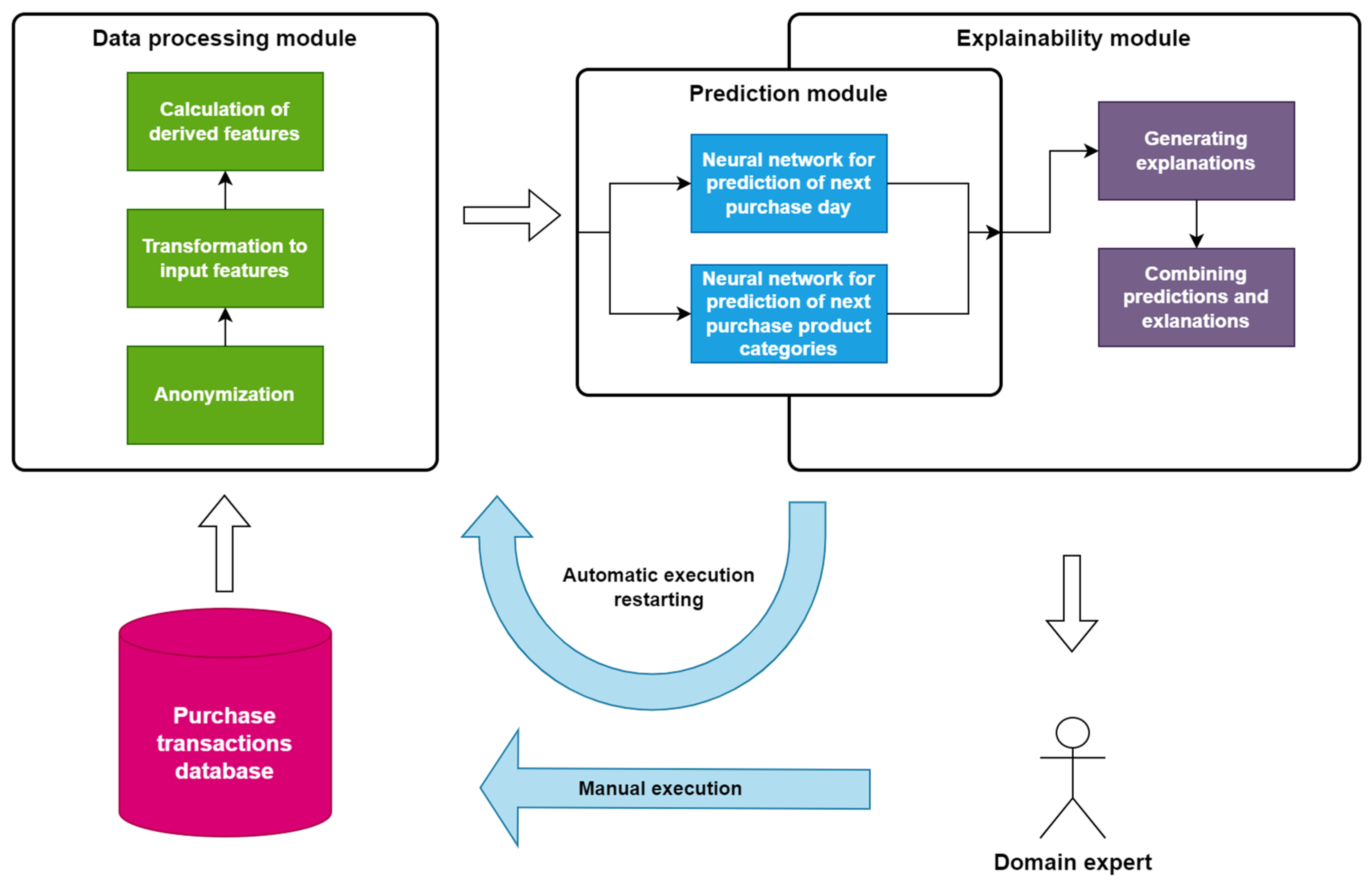
Figure 1 shows the proposed architecture of an explainable purchase prediction system for application in business. The system receives raw input data from the purchase transaction database. The data are usually in the form of a purchasing transaction, containing information such as customer identification, product(s) identification, time of transaction, purchased quantity, charged price, etc. Additional input data that is commonly available includes customer and product details. For customers, that could be location, age, and so on, while product information should at the very least include product categories.

Received data are first sent to the data processing module. This module performs three types of preprocessing:

• Anonymization—anonymization of all personally identifiable information present in raw data transactions
• Transformation to input features—transformation of the data to a format compatible with input features for a time series
• Calculation of derived features—generating derived input features from raw data that may increase the prediction accuracy

The resulting features are forwarded to the prediction module. Based on previous experience with purchase prediction [24], instead of a single multi-task neural network for predicting both the next purchase day and the next purchase product categories, two parallel single-task neural networks are contained in the Prediction module:

• A neural network for prediction of the next purchase day performs the task of predicting the day of the next purchase for a specific customer.
• A neural network for prediction of next-purchase product categories forecasts which product categories will be present in the following purchase by that customer.

While these two neural networks run in parallel, their structure and, especially, input features will differ in order to produce the highest possible accuracy.

Output values generated by the prediction module serve as input to the explainability module. This module is partially integrated with the prediction module since the neural networks are also needed to create explanations for single or multiple prediction instances. Explanations are usually produced in the form of diagrams that interpret predictions generated by the prediction model. Combined, predictions and explanations are the final output of the system that is given to the human user, i.e., the domain expert.

The user uses the system’s output to make business decisions and apply appropriate actions. The explanations provided alongside predictions enable the user to review predictions and question the logic behind them. Interpretation of the predictions helps the user see if they might agree with the conclusions given the additional information or if they will reject the system’s recommendation and rely solely on their own expert knowledge. The domain expert, as a system user, is in charge of any action taken.

The system is envisioned to be run regularly, once every predefined time period, e.g., once every week. Each time, new input data are acquired and used to retrain neural networks with new information. Only new data are used for additional training since everything else is already contained in the model. Besides automated execution at the end of the predefined time period, the user has the option to run manual execution at their own discretion.

Some examples of possible applications include procurement or production planning, encouraging the customer base to perform additional purchases, creating targeted personalized promotions, etc., [25,26]. A real-life application example and an implementation of the proposed architecture are described in the following section.

4. Implementation

In order to demonstrate the application of the proposed architecture, an implementation was built using the purchase prediction setup for a medical drug company. Input data are in the form of financial transactions for product purchases. The raw data are transformed into input features in the data processing module. The predictions about future purchases are then made in the Prediction module using LSTM neural network features with historical purchase transaction data. This information is then passed through the explainability module based on the SHAP library, where explanations for each prediction are generated. The combined results of the prediction and explainability modules are provided to the user to use in the business decision-making process. For evaluation of the implemented system, several regression metrics are used to compare three different implementations of the neural networks for prediction of the next purchase day.

4.1. LSTM Neural Network

Long-short-term memory neural networks are a type of recurrent neural network (RRN) initially proposed in [27]. The returning connections of the RNNs enable using the old cell state in addition to the new cell input, providing a memory of some sort. Over time, the influence of the older input fades, which is why long-term dependencies are a problem for RNNs. The main advantage of LSTM neural networks is their ability to store long-term dependencies in data, compared to RRNs. Although there are multiple proposed variations, the most important one is the introduction of the forget gate from [28], and this variation is the most commonly used to date.

Figure 2 shows the architecture of an LSTM cell. Each cell is a memory block that has three multiplicative gates: the input gate, the forget gate, and the output gate. These gates control which parts of the input, cell state, and output, respectively, will be used in further calculations and which parts will be discarded. The role of the input gate is to protect the memory content from irrelevant input [29], while the forget gate determines at what point to forget the previous state using resetting or gradual fading. The output gate prevents the cell state from perturbing the rest of the neural network.

The LSTM cell shown in Figure 2 can be described with Equations (1) to (5). In these equations, σ denotes the sigmoid function, while i, f, o, c, and x are activation vectors for the input gate, forget gate, output gate, cell, and cell input. The hidden vector is denoted with h, the biases with b, and the weight matrices with W. For each of the matrices, the subscript shows to which connection it applies.

$$i_t=\sigma (W_{xi}{x}_t+W_{hi}{h}_{t-1}+W_{ci}{c}_{t-1}+b_i),$$

(1)

$$f_t=\sigma (W_{xf}{x}_t+W_{hf}{h}_{t-1}+W_{cf}{c}_{t-1}+b_f),$$

(2)

$$c_t=f_t{c}_{t-1}+i_t\tanh (W_{xc}{x}_t+W_{hc}{h}_{t-1}+b_c),$$

(3)

$$o_t=\sigma (W_{xo}{x}_t+W_{ho}{h}_{t-1}+W_{co}{c}_t+b_o),$$

(4)

$$h_t=o_t\tanh (c_t),$$

(5)

4.2. Evaluation Metrics

For regression problems in machine learning, the goal is to predict a specific target value using independent variables. Performance fitness and error metrics used for regression rely on calculating point distance. The calculations are conducted on the values of actual measurements, predictions, and the number of data points by using subtraction and division, and sometimes absolute value and square roots. Although there are a great number of such metrics, most of the available research uses MAE, MAPE, RMSE, R, and R2 [30]. In this paper, mean absolute error (MAE), mean absolute percentage error (MAPE), and root mean square error (RMSE) are used to evaluate and compare different neural networks that are built for predicting the same output. All of these metrics represent the difference between the value predicted by the regression model and the actual value of that variable, but are calculated differently.

MAE represents the average of the absolute difference between the predicted value and the actual value. It is defined as:

$$MAE=\frac{1}{n}\sum _{t=1}^n\left|A_t-P_t\right|$$

(6)

MAPE is the average of the absolute difference between the predicted value and the actual value, divided by the actual value. It can be formulated as follows:

$$MAPE=\frac{1}{n}\sum _{t=1}^n\left|\frac{A_t-P_t}{A_t}\right|$$

(7)

RMSE is the square root of the average square difference between the predicted value and the actual value. It can be calculated with the formula:

$$RMSE=\sqrt{\frac{1}{n}\sum _{t=1}^n{(A_t-P_t)}^2}$$

(8)

In all the above formulas, n is the number of data points, while A_t and P_t are the values of the actual measurements and the predicted value for the data point t.

According to a review paper on error metrics [30], the characteristics of these metrics are:

• MAE is good for numeric data, uses a similar scale to input data, and enables comparing a series of different scales.
• MAPE works well with numeric data and is commonly used as a loss function, but it cannot be used if there are actual zero values.
• RMSE is scale-dependent, sensitive to outliers, and appropriate for numeric data; a lower value is more favorable.

Since all the aforementioned metrics correspond to the data and models in question, they were applied to the three neural networks for predicting the next purchase day.

The problem of predicting the number of days until the next purchase is a regression problem, but it can be reduced to a classification problem by discretizing predicted values into two classes:

• purchase is expected within the defined time period and
• purchase is not expected.

For classification problems, common metrics are accuracy, prediction, and recall [31]. Besides evaluating prediction results, they can also be used to compare the performance of different methods.

Accuracy is calculated overall for instances of all classes, while precision and recall are calculated for each of the existing classes. For any given class, precision is defined as the quotient of the number of correctly classified instances of that class and all instances that were assigned that class. Recall for a specific class is calculated as the quotient of the number of correctly classified instances of that class and the total number of instances belonging to that class. Finally, accuracy is defined as the quotient of the sum of all correctly classified instances (regardless of their class) and the total number of all instances. With all this in mind, it can be said that accuracy shows how often a model is correct for all classes, precision describes how often a model is correct in predicting a specific class, and recall represents how good the model is at finding all instances of a specific class.

Since one experiment phase includes reducing the regression problem to a classification one, appropriate classification metrics are used in the evaluation of the results of that phase.

4.3. SHAP

Shapley additive explanations (SHAP) values can be used to explain the output of a machine learning model by assigning each feature an importance value for a specific prediction [32]. SHAP is a game-theoretic approach based on optimal credit allocation and local explanations, utilizing classic Shapley values and their extensions.

For each of the input features, SHAP determines a change that the manipulation of that feature will render to the model’s prediction. The determined values indicate the path from the base value, i.e., the value that would be predicted without input features, to the actual predicted value. An illustration of this process is presented in Figure 3.

Shapley values are the solution to the equation.

$${\varphi }_i\left(f,x\right)=\sum _{z^{\prime }\subseteq x^{\prime }}\frac{\left|z^{\prime }\right|!\left(M-\left|z^{\prime }\right|-1\right)!}{M!}\left[f_x\left(z^{\prime }\right)-f_x\left(\frac{z^{\prime }}{i}\right)\right]$$

(9)

given that |z′| is the number of non-zero entries in z′, and z′ ⊆ x′ denotes z′ vectors for which the non-zero entries are a subset of non-zero entries in x′ and

$$f_x\left(z^{\prime }\right)={f(h}_x\left(z^{\prime }\right))=E[f\left(z\right)\left|z_S\right]$$

(10)

where S is the set of the non-zero indexes in z′.

Due to the complexity of the calculation, some simplifications and approximations are applied, leading to the final simplified computation of the expected values [32]:

$${f(h}_x\left(z^{\prime }\right))=E\left[f\left(z\right)|z_S\right]=E_{z_{\overline{S}}|z_S}[f\left(z\right)]\approx E_{z_{\overline{S}}}[f\left(z\right)]\approx f({[z}_S,E\left[z_{\overline{S}}\right]])$$

(11)

The approximation methods are model-agnostic and rely on feature independence and model linearity. According to [32], the SHAP framework identifies the class of additive feature importance methods and shows there is a unique solution in this class that adheres to desirable properties.

4.4. The BPPXL System

All processing components of the system were implemented in Python with the utilization of various libraries, including Pandas [33], Keras [34], TensorFlow [35], and SHAP [32].

The data processing module transforms acquired financial transactions into input features. The original data format contains customer and product identification, transaction date, product quantity, and separate additional product information, including the generic product identifier (GPI) [36], which is used for product categorization. The first step in data processing is anonymization, which removes all personally identifiable customer information. Since one of the input features for the LSTM neural networks is the period between two relevant purchases, the next step is the calculation of the derived features Period1, Period2, and Period3. Next, all transactions are aggregated by the purchasing customer. During this process, the GPI multi-hot encoded vectors are calculated for each purchase. The first hierarchical character group in the GPI therapeutic classification system enables the classification of drugs into 100 categories. The 99 categories are defined by GPI, and one additional category is created for products without available GPI information that make up around 2.5% of the total number of products. The resulting time series are generated in a format suitable for neural network training.

The prediction module consists of two parallel LSTM neural networks that simultaneously predict:

• product categories that will be a part of the following purchase and
• the timing of that purchase.

One LSTM neural network is designated for predicting the contents of the following purchase, i.e., the product categories that will be present in the next purchase. The prediction is generated in the format of a multi-hot encoded vector. In this vector, the value 1 at position i represents that the product category i is expected to appear in the following purchase, while the value 0 at position i represents that the product category i is not expected to appear in the following purchase.

The second LSTM neural network is tasked with predicting the time period until the next purchase. The different implementations of the second neural network were built and tested as part of this research:

• One univariate LSTM neural network that uses only the Peroid1 input feature with three time steps,
• One pseudo-multivariate LSTM neural network with two additional input features, Period2 and Period3, that are derived from the original univariate time series,
• One multivariate LSTM neural network that also includes the GPI category vector as its input feature.

Additionally, the neural networks were evaluated with two different activation functions. Combining the results from two parallel neural networks produces the full prediction of the time and contents of the following purchase for each of the customers. As the multivariate LSTM network with the relu activation function produced predictions with the highest accuracy, it was selected as the final choice for the BPPXL system implementation.

The explainability module interprets the predictions of the purchase day and produces several plot types for single-instance and multiple-instance predictions. The module is implemented by using the shap Python library using the post-hoc method, i.e., the explanations are generated for already trained models. For this reason, the explainability module is partially integrated with the prediction model. For each input feature, it attempts to attribute the significance of that feature to the predictions for the data samples. With this approach, the performance accuracy is preserved compared to a prediction system without the explainability module. Besides comparing the importance of individual features, the SHAP method gives the opportunity to compare different models focused on the same task. This is utilized to accentuate differences in three implementations of the purchase time prediction.

The interface integrates all outputs from the prediction and explainability modules and presents them to the user. This enables the user to review predictions and provide explanations. After receiving results, the user can make business decisions based on the generated results and their expertise. Besides automated execution of the system’s retraining and prediction process, there is also a possibility of manual execution by the user at any point in time. Some examples of possible applications and opportunities for decision making using the described system include:

• Product procurement planning based on the purchases predicted by the system,
• Personalized advertising directly to the customer, i.e., offering better buying conditions in the case of a purchase or reminding a customer they forgot to order some products,
• Detecting lost customers, i.e., customers who have switched to a different supplier, based on a mismatch between predicted and actual behavior.

The system is initially trained and run, and then periodically retrained with additional transactions to always make predictions based on the newest information. Initial training can be long if there is an exceptionally large amount of training data. However, retraining is only performed with newly available data at regular time intervals, which shortens the training time considerably. After a defined period (e.g., 10 years), some purchasing data can be declared outdated and eliminated from the training set if that is necessary. Another possibility when an excessive amount of data are available is the consolidation of smaller periods prior to training.

5. Experiments

The experiments were conducted in three phases. In the first phase, the three purchase time prediction neural networks were evaluated using two different activation functions: tanh, which is the default activation function for the LSTM layer in Keras, and relu. The evaluations were performed using the common regression metrics MAE, MAPE, and RMSE. The results of these evaluations are shown in

Table 1. Prediction results using regression metrics for three neural networks for purchase time prediction using the tanh activation function.

Purchase Time Prediction NN	MAE	MAPE	RMSE
Univariate LSTM	20.68	44.49%	84.74
Pseudo-multivariate LSTM	19.14	36.74%	82.15
Multivariate LSTM	16.42	10.02%	80.74

for the experiments using the tanh activation function and

Table 2. Prediction results using regression metrics for three neural networks for purchase time prediction using the relu activation function.

Purchase Time Prediction NN	MAE	MAPE	RMSE
Univariate LSTM	20.99	49.15%	84.17
Pseudo-multivariate LSTM	3.38	26.76%	18.00
Multivariate LSTM	0.19	2.16%	0.72

for the experiments using the relu activation function.

The data used for training and evaluation was acquired from a medical device and drug vendor and contains around 7.5 million transactions. Each transaction includes a customer identifier, a product identifier, a product quantity, and the date and time of the transaction. Customer orders usually consist of multiple products, but each is recorded separately in the system’s database. Auxiliary information about products is available in an additional table, the most significant being the GPI value. In all orders, around 11,000 different products appear. Only around half of the products initially had assigned GPI values, but based on other product information, it was possible to fill in at least the first 4 to 8 characters for 97.5% of the products. According to the first hierarchical group of the GPI value for each product, an appropriate product category (one of the potential 100) was assigned.

The first step in preprocessing consisted of aggregation by customer, followed by calculation of derived features. After aggregation and removing customers with too few orders for feature calculations, the resulting dataset contained around 1 million orders with multiple products in each order. The orders were made by a little over 10,000 customers, with the majority of customers making 200 or fewer orders.

Several observations can be made based on the results from Table 1 and Table 2. First, the more neural networks with a greater number of input features, the better their prediction accuracy, regardless of the activation function used. However, when using the tanh activation function, the increase in performance might not be sufficient to justify the use of more input features. The input feature for the univariate LSTM neural network is the easiest to calculate and requires the fewest number of purchases per customer in order to be able to use transactions for that customer. All other features take significantly longer to be calculated.

It can also be noticed that for a univariate LSTM neural network, both activation functions lead to similar results. On the other hand, for pseudo-multivariate LSTM neural networks and multivariate LSTM neural networks, all metrics are greatly improved when using the relu activation function.

The absolutely superior results are achieved using the multivariate LSTM neural network utilizing a relu activation function that has as its input features Peroid1, Period2, Period3, and a multi-hot encoded GPI category vector, with each element denoting the presence of one of the 100 product categories. This network structure was chosen as the final implementation for the BPPXL system due to its highest prediction accuracy.

In the second phase of the experiments, the problem of purchase time prediction was considered a classification problem with the goal of examining accuracy prediction in this approach. In predicting the following purchase timing, the exact number of days until the purchase may be irrelevant. Instead, it is important to determine if the purchase will occur within the defined time period or not. In this case, the time period was defined as a week, i.e., 7 days. All prediction values up to 7 can be considered an expected purchase, while those that are greater than 7 indicate that the purchase is not expected. For evaluation purposes, these two classes were labeled “Realized Purchases” or RP, and “Unrealized Purchases” or UP. After reducing the problem to a classification one, the classification metrics accuracy, precision, and recall were applied to the prediction results.

Table 3. Prediction results using classification metrics for three neural networks for purchase time prediction using the tanh activation function.

Purchase Time Prediction NN	Accuracy	Precision RP	Recall RP	Precision UP	Recall UP
Univariate LSTM	77.74%	76.39%	96.63%	85.23%	39.44%
Pseudo-multivariate LSTM	86.56%	86.05%	95.41%	88.05%	68.63%
Multivariate LSTM	95.59%	99.67%	93.72%	88.64%	99.38%

and

Table 4. Prediction results using classification metrics for three neural networks for purchase time prediction using the relu activation function.

Purchase Time Prediction NN	Accuracy	Precision RP	Recall RP	Precision UP	Recall UP
Univariate LSTM	75.49%	74.94%	95.25%	78.62%	35.4%
Pseudo-multivariate LSTM	88.41%	89.24%	95.06%	87.89%	77.02%
Multivariate LSTM	95.79%	99.84%	93.87%	88.92%	99.69%

show classification metrics values for purchase time prediction using the tanh and relu activation functions, respectively.

Compared to experiments with regression metrics, the similarity is the fact that the univariate LSTM neural network tanh activation function produces slightly better results. For the pseudo-multivariate LSTM neural network and the multivariate LSTM neural network, generally, the opposite is true. However, it should be noted that the difference between prediction accuracies is not significant with different activation functions, while the difference for regression metrics is quite drastic. It can be concluded that, depending on the specificity needed, the choice of the activation function may be more or less important.

More complex neural networks with more input features are superior as well in predicting the purchase time with a classification approach. Using this approach, the improvement of the prediction metrics is quite visible and relatively similar for both activation functions.

It can be concluded that the multivariate LSTM model was the most successful in both the regression and classification approaches. This model is trained with the largest number of input features related to past purchases, which is probably the most significant reason for the beastly performance of this neural network in all cases.

In the regression case, the choice of the activation function has proved to be very consequential. The highest performance was achieved with the relu activation function. This relu function introduces the property of non-linearity to machine learning models and solves the vanishing gradient problem. This is the most probable reason for the increase in all metrics when using this activation function. On the other hand, in the classification approach, there was no significant difference in performance when using different activation functions.

The third and final phase of experiments consisted of applying the explainability module to three developed neural networks for predicting purchase time. For this experiment, several types of plots were generated for single and multiple instances. The explainability plots were generated solely for LSTM neural networks with relu activation functions since they outperformed their tanh activation function counterparts.

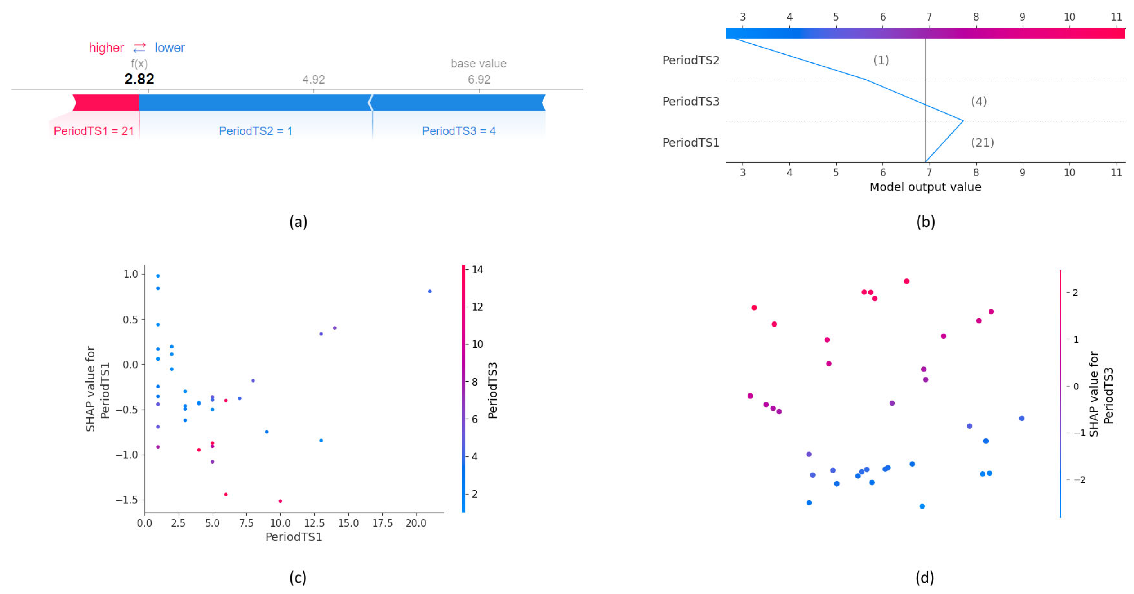
For each of the neural networks, multiple types of plots were generated, specifically force plots, decision plots, dependance plots, and embedding plots for each of the input features. Figure 4 shows all the types of plots used for selected instances of the univariate LSTM (ULSTM) neural network for purchase time prediction. This neural network is chosen for illustration because it has the most clearly visible representation due to its smallest number of features. Since the time series for each of the neural networks had three time steps, in SHAP plots, each time step is shown as a separate feature.

A force plot shows how each of the features contributes to the prediction for a single instance. It is also possible to generate force plots for multiple instances. The base value is the value that the model would predict without the impact of the features, and the actual predicted value is marked as f(x). The features are shown in red and blue, with red representing features that contribute to the predicted value being higher and blue representing features that affect the predicted value being lower. Features with the greatest influence are shown closer to the predicted value, and their representations are larger. An example shown in Figure 4a shows that for a base value of 6.92 and respective property values 21, 1, and 4 from three time steps, the feature with the value 21 pushes for the prediction value to be higher, while the other two features influence the prediction value to be lower. From the sizes of the feature representations, it is obvious that the two features lowering the prediction value have a greater impact, which results in an actual prediction value of 2.82.

The decision plot presents similar information as the force plot, but perhaps more clearly. The force plot can also be created for a single or multiple instances. The vertical line is positioned at the base value, and the polyline starts at the base value and finishes at the actual predicted output. The path of the polyline is determined by the input features whose values are shown. Longer segments represent features with a greater influence on the predicted value. The example in Figure 4b makes it evident that the feature PeriodTS1 with the value 21 attempts to make the predicted value higher, while the other two features try (and succeed) to lower the predicted value.

A dependence plot or partial dependence plot shows the effect that one or two features have on the model’s predicted value with the assumption that the features are not correlated. Unlike the previous two plots, this one is created for multiple instances to visualize the global correlation of a feature and the model’s prediction value. It is a scatter plot in which a dot represents a single prediction, the x and y axes represent the feature value and the SHAP value for that feature, respectively, and the color of the dot is determined by the second feature. A vertical color pattern suggests that the two features have an interaction effect. In Figure 4c, the dependence plot for features PeriodTS1 and PeriodTS3 is shown. The blue color of almost all the dots corresponding to the PeriodTS1 value under 2.5 indicates that an interaction effect exists between these two features.

Embedding plots project SHAP values to 2D using PCA for visualization, and they are also generated for a single feature and multiple instances. These plots enable the user to see the spread of SHAP values for a specific input feature. The impact of the feature can be seen in the intensity of SHAP values and the clustering of positive and negative SHAP values [37]. The model’s predicted values are clustered by explanation similarities. Figure 4d shows the embedding plot for the feature PeriodTS3, which has evident clustering of positive and negative values.

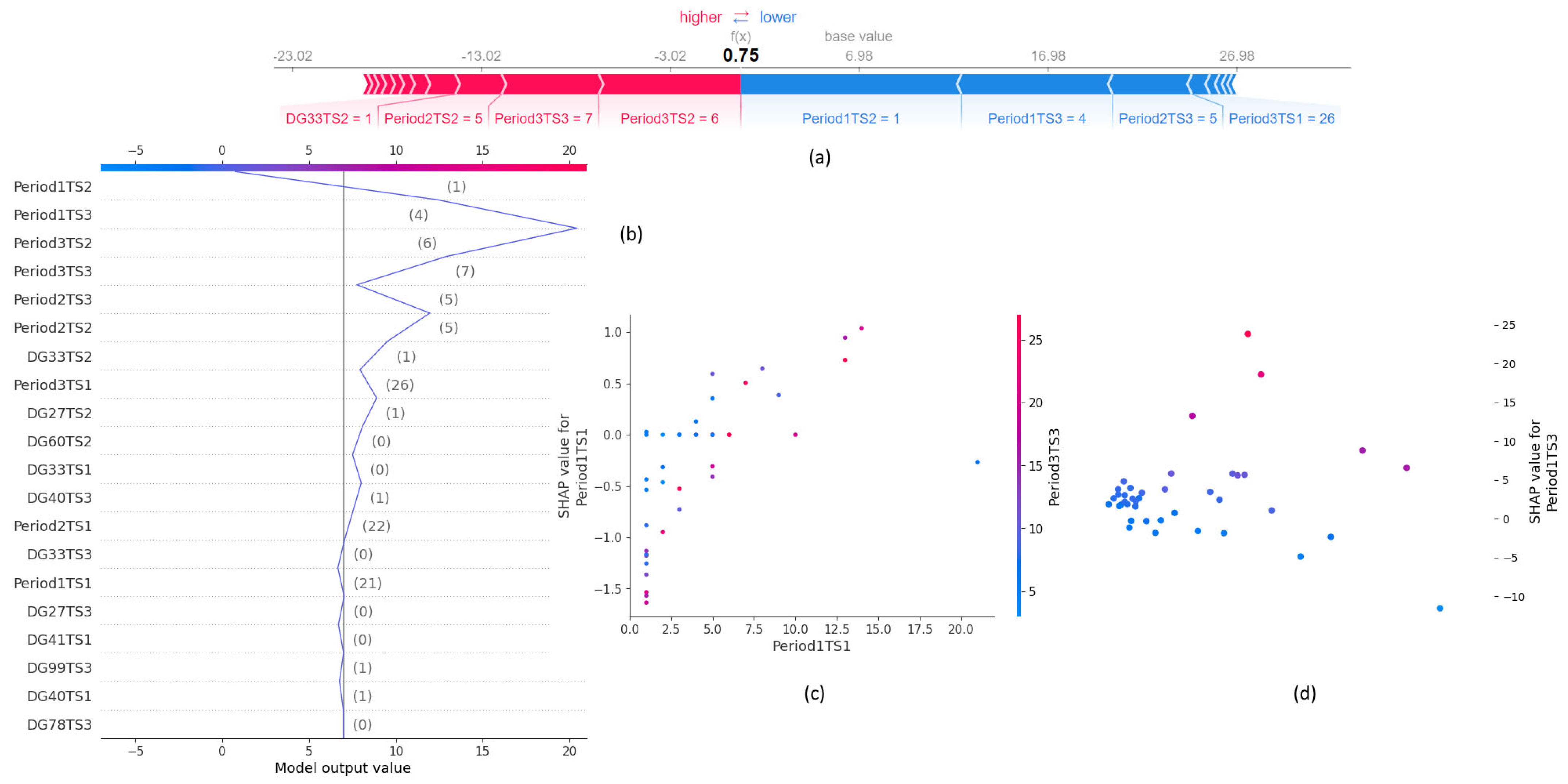
Figure 5 and Figure 6 show examples of all types of plots for the pseudo-multivariate LSTM (PMLSTM) neural network for purchase time prediction and the multivariate LSTM (MLSTM) neural network for purchase time prediction, respectively. Force and decision plots are plotted for the same instance, while dependence and embedding plots are generated for the corresponding features to the features represented in these plots in Figure 4.

In Figure 5a,b it is noticeable that additional features of the PMLSTM neural network have greater importance for the model’s prediction, while features that also exist in the ULSTM have a smaller impact. While the dependence plot shown in Figure 5c has similarities with the plot in Figure 4c, indicating an interaction effect, the second plotted feature is not the same for these two plots, making comparison difficult. Unlike the embedding plot for ULSTM, in Figure 5d there is no definitive clustering to signify the feature effect.

For the MLSTM, the force and decision plots from Figure 6a,b show that, despite the great number of features added, the most significant features for the prediction result are those that are also present in the ULSTM. Here, there are no similarities between the dependance plots for the feature Period1TS1 shown in Figure 6c and neither of the dependence plots for ULSTM or PMLSTM. However, there is a clear clustering of SHAP values, especially negative ones, in the plot shown in Figure 6d, indicating that the feature Period1TS3 notably influences the prediction value for the MLSTM model.

6. Conclusions

In this paper, an architecture of a machine learning time series prediction system based on LSTM neural networks and enhanced with XAI techniques is proposed. The architecture is implemented on an example of a system for prediction of following purchases for business time series containing financial transaction data by predicting the day and product categories for the next purchase of each customer. The BPPXL system enables the prediction of the following purchases for business time series containing financial transaction data by predicting the day and product categories for the next purchase by each customer. The use of LSTM neural networks results in high prediction performance, while explainability provides transparency for humans working with the system, thus increasing confidence in the system. This system was developed using data collected from a medical device and drug vendor; however, it can be adapted for any B2B system in which products can be divided into an appropriate number of specific categories. The main contribution of the work presented in this paper is developing the architecture of a system that includes the explainability component that allows the human user (a domain expert, usually a business analyst) to understand the system’s decisions. Interpretation provided by the XAI component builds the user’s trust, which is crucial if that user is expected to rely on system recommendations in making business decisions. Additionally, an implementation of the XAI component based on the SHAP library was developed and tested with three different LSTM neural networks for predicting the next purchase day. The three selected networks have different input features and structures and consequently produce predictions of various accuracy. Integration of the XAI module with each of the neural networks results in the creation of explanations that interpret the neural network prediction and are attached to the provided prediction as the system output. One additional potential benefit of the enhanced XAI output of the system is the ability to analyze the significance and impact of individual features of the resulting predictions. These findings can be used to optimize the system by pruning input features with minimal effect on the system output, retaining only the most significant features. Models with fewer and more significant features might be able to produce comparatively high accuracy while improving efficiency, i.e., reducing training time and achieving the ability to produce predictions in real time.

The use of GPI hierarchical classification for product categories is a limitation of the implemented system since it restricts its application to the medical drug industry. On the other hand, the proposed architecture defines a blueprint for developing a specialized system that will be more suitable for a specific real-life application.

One potential direction for future work is extending the proposed architecture with the introduction of the module tasked with validating predictions from the previous time period using newly available input data. This module can then be used for system optimization.