Adaptive Fractional Prescribed Performance Control for Micro-Electromechanical System Gyros Using a Modified Neural Estimator

Abstract

In this paper, a neural fractional order prescribed performance control is proposed for micro-electromechanical system (MEMS) gyros. Gyros tend to become smaller in size and more precise in structure with the development of micro-manufacturing technology. The operational security for MEMS gyros in cases of disturbances and parameter uncertainties becomes a challenging problem that has attracted much attention. The proposed method incorporates a prescribed performance technique to accomplish a bounded (within 10% of the vibration amplitude) gyro trajectory tracking error dynamic to secure the gyro’s operation. Meanwhile, fractional calculus is integrated into the controller’s design to provide precise adjustments to the gyro’s motion and thus further improve gyro control performance (shortening error convergence time by 20%). Furthermore, to enlarge the application scope and to improve gyro system robustness, a modified neural network estimator with a constrained input mapping mechanism is proposed to approximate unknown time-varying angular-velocity-related gyro dynamics. Notably, the constrained input mapping mechanism can help guide neural parameter initialization to avoid a time-consuming parameter adjustment process. The stability of the closed-loop gyro control system is proved in the framework of Lyapunov stability theory, and comparisons of simulation results are presented to demonstrate the effectiveness of the proposed method.

1. Introduction

As one kind of inertial navigation device, the gyroscope has attracted great and increasing attention from researchers and engineers ever since it was first invented circa the 1800s. With the development of navigation in drones and many other consumer electronic devices, the gyroscope has gradually become one of the most important gesture-detecting sensors used to provide angular velocity measurement. As far as the authors know, there are various kinds of gyroscopes, such as the mechanical gyroscope, the optical gyroscope, the gas-bearing gyroscope, and so on. Different gyroscopes are quite different in their features as well as in their operational principles. Among the gyroscopes mentioned above, the MEMS gyroscope is one of the most advanced angular velocity-detecting sensors and is continuously penetrating into application areas to replace traditional types of gyroscopes due to its prominent advantages such as small size, low cost, easy implementation, and so on [1,2,3].

The principle that the gyroscope can measure angular velocity is based on the “Coriolis effect” in which a mass tends to move to the left of its direction of motion when the plane on which the mass is moving undergoes a clockwise rotation. The generated force that causes the mass to deflect from its original motion direction is the “Coriolis force”, and the force is proportional to the rotation speed [4]. To provide stable and accurate angular-velocity information, the proof mass in the gyroscope is firstly driven into a sinusoidal vibration mode along an axis named the “driving axis”. The proof mass will then be pulled to vibrate by the Colioris force along the axis perpendicular to the “drive axis” named the “sensing axis”. Information relating to the applied angular velocity can be extracted by detecting the vibration amplitude of the proof mass in the sensing direction [5]. In practical MEMS gyro control methods, feedback-control techniques (especially adaptive gain control and phase-lock loop) are mostly adopted to control the vibration amplitude and the phase of the proof-mass trajectory [6]. Actually, this kind of single-axis feedback control scheme works well in driving the proof mass into a desired trajectory, and the methods are widely utilized in applications without severe precision or robustness requirements like consumer electronics. The main factor hindering this kind of single-axis control method from acquiring better gyro performance lies in the structure of the control scheme in which no control force is applied in the sensing direction [7,8]. In this structure, even a very mild disturbance can cause unneeded movement of the proof mass in the sensing axis, and this “false” movement can directly lead to false angular velocity output, degrade measuring precision, or even cause sensing components (capacity combs) to collide, resulting in damage to the gyroscope. To achieve a satisfactory driving mode oscillation, researchers have devoted considerate efforts to the control of gyros, and various advanced control methods have also been applied to it [9,10].

As one kind of robust control scheme, sliding mode control (SMC) is superior in its control performance in dealing with external disturbances as well as parameter uncertainties. At the same time, the MEMS gyro, as one kind of complex and precise measurement device, can be easily affected by external and internal disturbances. As a result, it is natural and feasible to use SMC in the control of the gyro’s dynamics, and relevant approaches have been developed. In [11], a harmonic disturbance observer is integrated into the SMC for gyro control, in which the frequency information is used to achieve high tracking accuracy. A compound control method for gyro control integrating PD control and terminal SMC is introduced in [12], achieving finite time tracking error convergence as well as strong robustness. However, the traditional SMC methods mentioned above cannot avoid chattering in control forces, and the high-frequency chattering can cause damage to actuators in gyros. To make up for this drawback, investigations such as high-order sliding mode control [13], the super twisting algorithm [14], and so on have been vastly and deeply investigated for chattering reduction.

To further improve gyro vibration qualities and to enhance the security of the gyro’s operational mode, research efforts on transient and steady-state gyro tracking error performance have attracted increasing attention [15,16,17]. In [18], a backstepping control technique is adopted for gyro control, in which the stability of the entire control system is proved using a barrier Lyapunov function, which can guarantee that gyro vibration amplitudes are constrained to evolve within predefined limits. In [19], a prescribed performance-control technique is used to maintain predetermined performance constraints on gyro tracking dynamics, and several methods, like event-trigger mechanism, fault-tolerant control, and terminal sliding control, are incorporated to achieve several outstanding accomplishments [20,21,22]. The above-mentioned works mainly concentrate on gyro-control performance under constant angular velocity, while cases under time-varying angular velocity have rarely received attention.

In recent decades, artificial intelligence techniques have undergone rapid development, and AI development has also contributed to the evolution of control research. In general, control for systems subjected to unknown dynamics is a challenging problem, but artificial intelligence techniques such as the neural network and fuzzy logic have provided easy and feasible solutions for this kind of control issue [23,24,25]. In gyro control using neural network techniques, generally speaking, the approximation capacity of neural networks is usually adopted in two main aspects, disturbance approximation (including the value of disturbance or disturbance bound) [23,24] and gyro dynamic approximation (including unknown system functions or gyro system parameters) [25]. The results show that neural network technology is functional and plays a crucial role in corresponding gyro controller designs. However, as far as the authors know, selection for neural network parameters is of significant importance in neural network approximation performance. Improper parameters can degrade approximation performance in terms of settling time and accuracy. How to choose proper/optimal neural network parameters so that the neural network approximation capacity can be fulfilled remains unsolved, given that parameter adjustments still mainly rely on the rule of thumb or the trial-and-error method.

In summary, although the aforementioned studies have deeply and vastly studied the control methods for gyros, and technical developments in the gyro industry have also been greatly accelerated during the recent decades, there is still room for improvement, especially in the investigation of neural-network-based control for the safe operation of gyros subjected to continuously time-varying angular velocity.

In this paper, our goal is to ensure a safe and satisfactory operation of MEMS gyros in the presence of time-varying angular velocity. The idea of integrating modifications to neural networks with fractional order prescribed performance control is formulated. In the proposed control scheme, a constrained error mapping mechanism is designed and embedded in a neural estimator to derive a good approximation of the gyro unknown dynamic. Meanwhile, fractional calculus is utilized in the prescribed performance control to provide more flexibility in the controller design. In comparison with existing results, the main advantages of the proposed method can be summarized as follows:

• A constrained signal mapping mechanism is introduced to map the input signals of the neural network into a predefined range with a fixed boundary, which can thus guide neural network parameter initialization.
• A modified neural network-based estimator is proposed to dynamically estimate gyro dynamics, and the neural estimator is incorporated into the prescribed performance control structure to ensure safe gyro operation under time-varying angular rates. The proposed control method thereby has a broader range of applications.
• Fractional calculus is integrated with the proposed adaptive neural prescribed performance method to provide more flexibility in adjusting gyro dynamics. The involvement of fractional calculus in the controller design as well as the adaptive laws can jointly contribute to the overall quality of gyro vibration performance.

The remainder of this paper is organized as follows: In Section 2, a dynamic model of a simplified MEMS gyroscope system is introduced. In Section 3, the design of the adaptive prescribed performance control with a modified neural estimator is provided, and the proof of the stability of the gyro control system is also given in this section. Section 4 presents the simulation results and Section 5 gives the conclusion.

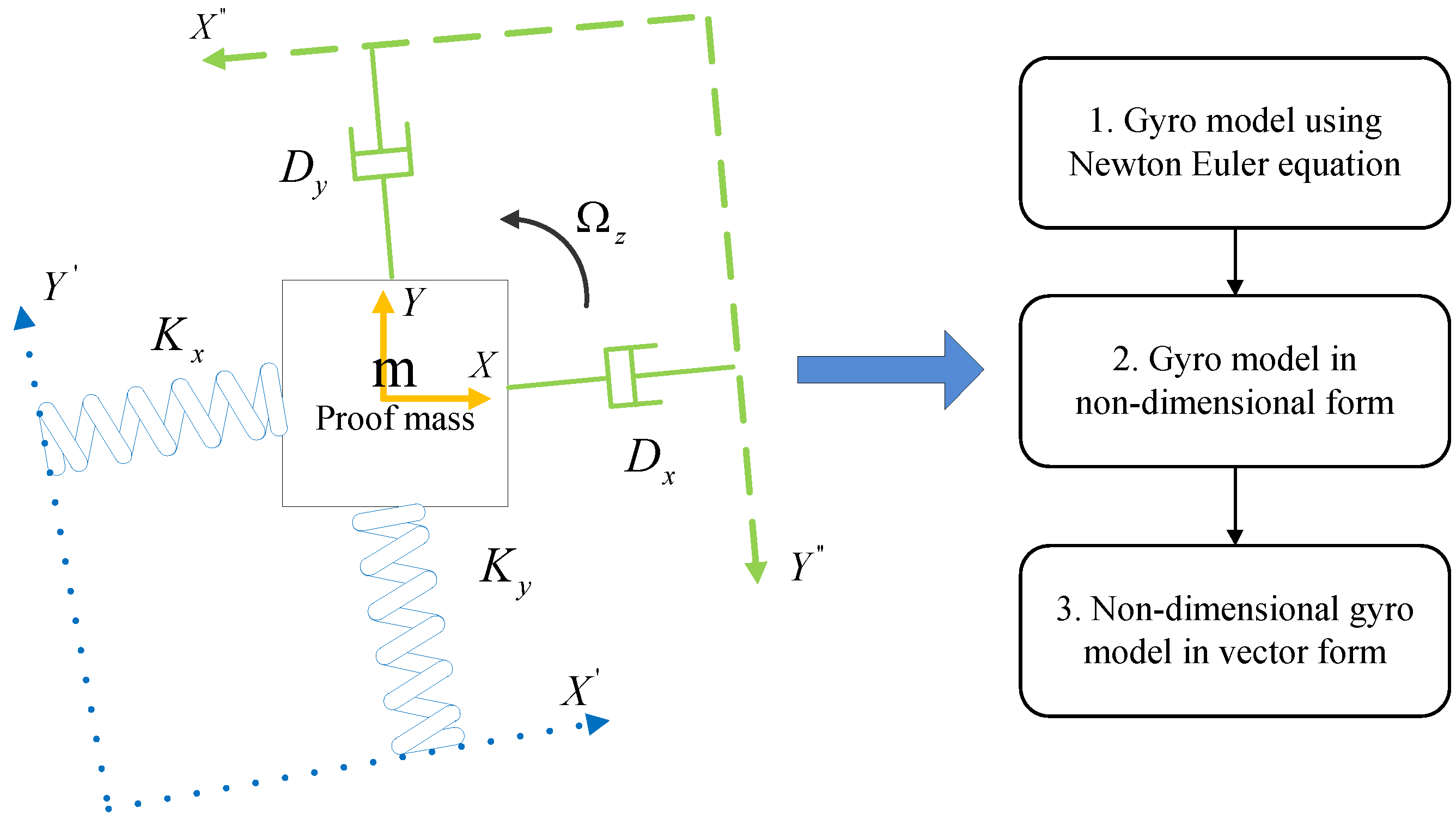
2. Structure and Dynamic of Z-Axis Vibrating Gyro System

The structure of a single-axis MEMS vibratory gyroscope can be simplified as a vibratory system consisting of a proof mass, springs, and dampers. As depicted in Figure 1, the proof mass is suspended by two sets of springs and dampers, where the mass is constrained only to move in the X-O-Y plane. One can easily drive the mass to vibrate in the X-axis while the mass remains still in the Y-axis if no angular velocity is applied to the gyro. If the gyro undergoes some rotation along the Z-axis, which is perpendicular to the X-O-Y plane, the proof mass will be pulled and pushed by the generated Coriolis force, resulting in the vibration of the mass in the Y-axis. Simultaneously, the mass displacement in the Y-axis is proportional to the applied angular velocity. One can easily obtain the value of the angular velocity by using the detected information of the displacement of the proof mass in the Y-axis.

However, all the results mentioned above are based on the assumption that the gyro structure is completely symmetrical; more specifically, the suspending springs and the dampers can perfectly and completely align with the motion axes. In this perfect mechanical gyro structure, the suspending frame coordinates (X′-O-Y′ and X″-O-Y″) can completely overlap with the motion coordinate (X-O-Y), and there is no other force except the Colioris force that can cause the mass to vibrate in the Y-axis. Despite the rapid development of advanced manufacturing technologies, the MEMS gyro structure can never be perfectly symmetrical, and there always exists some angle deviation between the suspending frame coordinate and the motion coordinate. The asymmetrical structure can result in displacement of the proof mass in the Y-axis even if the gyro is not rotating at all. Following the modeling steps depicted in Figure 1, the following Newton–Euler equation can be derived to describe the dynamics of the gyro in the presence of angular deviation between the coordinates [26,27].

$$\left\{\begin{array}{l}m\ddot{x}+D_{xx}\dot{x}+D_{xy}\dot{y}+K_{xx}x+K_{xy}y=u_x+2m{\mathrm{\Omega }}_z\dot{y}+F_x\\ m\ddot{y}+D_{xy}\dot{x}+D_{yy}\dot{y}+K_{xy}x+K_{yy}y=u_y-2m{\mathrm{\Omega }}_z\dot{x}+F_y\end{array}\right.$$

(1)

where $m$ is the weight of the proof mass; $x$ and $y$ are the displacements of the mass in the X and Y directions; $K_{xx}$, $K_{yy}$, $D_{xx}$, and $D_{yy}$ are the spring stiffness coefficients and damping coefficients in the X and Y directions; $D_{xy}$ and $K_{xy}$ are the coupling coefficients due to the asymmetric structure; ${\mathrm{\Omega }}_z$ is the angular velocity, and $u_x$, $u_y$ and $F_x$, $F_y$ are control forces and disturbances in the X and Y directions.

One can obtain the motion equations in non-dimensional form by dividing both sides of (1) by a reference weight $m$, length $q_0$, and resonance frequency ${\omega }_0^2$ for easy mathematical calculation. The non-dimensional gyro dynamic equation [26,27] is given as

$$\left\{\begin{array}{l}\ddot{\overline{x}}+{\overline{d}}_{xx}\dot{\overline{x}}+{\overline{d}}_{xy}\dot{\overline{y}}+{\overline{K}}_{\mathrm{xx}}\overline{x}+{\overline{K}}_{\mathrm{xy}}\overline{y}={\overline{u}}_x+2{\overline{\mathrm{\Omega }}}_z\dot{\overline{y}}+{\overline{F}}_x\\ \ddot{\overline{y}}+{\overline{d}}_{xy}\dot{\overline{x}}+{\overline{d}}_{yy}\dot{\overline{y}}+{\overline{K}}_{\mathrm{xy}}\overline{x}+{\overline{K}}_{\mathrm{yy}}\overline{y}={\overline{u}}_y-2{\overline{\mathrm{\Omega }}}_z\dot{\overline{x}}+{\overline{F}}_y\end{array}\right.$$

(2)

where $\overline{x}$ $\overline{y}$ ${\overline{K}}_{xx}$${\overline{K}}_{yy}$${\overline{D}}_{xx}$${\overline{D}}_{yy}$${\overline{D}}_{xy}$${\overline{K}}_{xy}$ ${\overline{\mathrm{\Omega }}}_z$${\overline{u}}_x$ ${\overline{u}}_y$ ${\overline{F}}_x$ and ${\overline{F}}_y$ are the corresponding displacements, gyro parameters, control forces, and disturbances derived through the nondimensionalization.

We can rewrite the gyro motion equation in vector form [26,27] as

$$\ddot{q}+D\dot{q}+Kq=U-2\mathbf{\Omega }\dot{q}+F$$

(3)

where $q=\left[\begin{array}{c}\overline{x}\\ \overline{y}\end{array}\right]$, $U=\left[\begin{array}{c}{\overline{u}}_x\\ {\overline{u}}_y\end{array}\right]$, $D=\left[\begin{array}{cc}{\overline{d}}_{xx}& {\overline{d}}_{xy}\\ {\overline{d}}_{xy}& {\overline{d}}_{yy}\end{array}\right]$, $K=\left[\begin{array}{cc}{\overline{K}}_{\mathrm{xx}}& {\overline{K}}_{\mathrm{xy}}\\ {\overline{K}}_{\mathrm{xy}}& {\overline{K}}_{\mathrm{yy}}\end{array}\right]$, $\mathbf{\Omega }=\left[\begin{array}{cc}0& -{\overline{\mathrm{\Omega }}}_z\\ {\overline{\mathrm{\Omega }}}_z& 0\end{array}\right]$, and $F=\left[\begin{array}{c}{\overline{F}}_x\\ {\overline{F}}_y\end{array}\right]$.

Here, the disturbance is assumed to be bounded such that $F\le F_d({\overline{F}}_x\le {\overline{F}}_{xd},{\overline{F}}_y\le {\overline{F}}_{yd})$. We aim to achieve the following objectives in this study: (1) drive the proof mass into a “driving” mode so that the proof mass trajectory can successfully track a given trajectory; (2) ensure that the trajectory tracking error evolves only in a predefined boundary to secure the safe operation of the gyroscope; and (3) correctly and in real time estimate the gyro dynamics containing the applied angular velocity.

3. Design of Adaptive Fractional Neural Prescribed Performance Control for MEMS Gyro

3.1. Prescribed Performance Control for Gyro Using Fractional-Order Sliding Manifold

Considering the presence of the various disturbances and system parameter uncertainties in the gyro system, it is logical and feasible to utilize a sliding mode control scheme for the control of gyros due to its notable robustness and so on.

The tracking error of the proof mass and its derivative are defined as

$$e=\left[\begin{array}{c}{e}_x\\ e_y\end{array}\right]=q_r-q$$

(4)

$$\dot{e}=\left[\begin{array}{c}{\dot{e}}_x\\ {\dot{e}}_y\end{array}\right]={\dot{q}}_r-\dot{q}$$

(5)

where $q_r=\left[\begin{array}{c}{q}_{rx}\\ q_{ry}\end{array}\right]$ is the reference trajectory vector with $q_{rx}$ and $q_{ry}$ standing for the desired trajectory that the proof mass shall be driven to follow in the X and Y directions. $e_x$ and $e_y$ are the position tracking errors in the X and Y directions, respectively.

The primary objective of controlling MEMS gyroscopes is that the proposed control method can accurately drive the proof mass to track a desired command trajectory. Due to the presence of various disturbances in measuring occasions, a sudden collision or shock may lead to a deviation in the actual trajectory of the proof mass from the command trajectory. However, the quality of the vibration mode is crucial for a vibratory gyroscope, as a degraded quality of the driving mode can seriously impact the performance of angular velocity measurement. Furthermore, an excessively large displacement of the proof mass may cause the detecting capacity combs to collide, potentially causing damage to the gyroscope itself. To improve the quality of the driving mode and to avoid damage to the gyroscope, it is essential to carefully monitor and control the vibration amplitude, keeping it strictly within a predefined bound so that detecting capacity combs mounted upon the proof mass will not collide with the fixed capacity combs on the suspending framework.

To enhance the safety of the vibration mode, the PPC control technique can be integrated into conventional control methods to apply constraints on gyro vibration dynamics. The following steps are introduced to obtain the equivalent unconstrained error through error transformation.

Firstly, since gyro vibration is one kind of simple symmetrical harmonic motion around the origin point along the driving axis, a symmetrical performance bound is established to impose a specific constraint on the gyro vibration. As stated in the work of Charalampos and Rovithakis [28], a function can be used as a performance function if it can meet the following three requirements: (a) the function is continuous and derivable; (b) the function is independent of system states while it can vary with time; and (c) the function is monotonously decreasing with time.

Here, an exponential function is chosen as the performance function in the following form.

$$p(t)=(p_0-p_{\infty })e^{-lt}+p_{\infty }$$

(6)

where $p_0$ $p_{\infty }$ and $l$ are appropriate positive constants, $p_0=p(0)$ specifies the initial maximum allowable tracking error boundary, $p_{\infty }=\underset{t\to \infty }{\lim }p(t)$ specifies the maximum allowable tracking error boundary at steady states, and $l$ is the adjustment factor associated with the decreasing rate of the performance function.

Prescribed performance is achieved if system tracking errors strictly evolve within the designed boundary. For the gyros, the tracking error that conforms to the prescribed performance can be described by the following constraint inequality.

$$\underset{\_}{p}(t)<e(t)<\overline{p}(t) \left( \forall t\ge 0,\underset{\_}{p}(t)=-p(t),\overline{p}(t)=p(t)\right)$$

(7)

Remark 1. 

A MEMS vibrating gyroscope can be simplified as a symmetrical spring-damper-mass vibrating structure. The vibration of the proof mass is a symmetrical vibration motion about the central point of the gyroscope structure in both the driving and sensing axes. As a consequence, a corresponding symmetrical error boundary is chosen in this study.

Then, to address the error constraint denoted by the inequality (7), an error index is introduced in conjunction with a corresponding transformation function. The transformation function can convert the prescribed performance characteristic from a constrained form to an unconstrained form. Consider the error transformation function in the form

$$\frac{e\left(t\right)}{p\left(t\right)}=\mathrm{\Theta }\left(\psi \right)$$

(8)

In accordance with the performance constraint imposed on gyro system tracking errors, the range of the transformation function is chosen such that $-1<\mathrm{\Theta }\left(\psi \right)<1$ for any value of $\psi$. To match the upper and lower bound values of the transformation function, a hyperbolic tangent function is utilized in the design procedure to connect the original tracking error and the transformed equivalent error.

$$\frac{e\left(t\right)}{p\left(t\right)}=\mathrm{\Theta }\left(\psi \right)=\frac{1-e^{-\mathrm{\sigma }\psi }}{1+e^{-\mathrm{\sigma }\psi }}$$

(9)

where $\mathrm{\sigma }$ is the adjustment factor used to change the shape of the function.

One can further obtain the transformed equivalent error by solving the inverse function of the transformation function; the derived equivalent error is given as

$$\psi ={\mathrm{\Theta }}^{-1}(\frac{e\left(t\right)}{p\left(t\right)})=-\frac{1}{\mathrm{\sigma }}\ln \left(\frac{1+\frac{e\left(t\right)}{p\left(t\right)}}{1-\frac{e\left(t\right)}{p\left(t\right)}}\right)=-\frac{1}{\mathrm{\sigma }}\ln \left(\frac{p\left(t\right)-e\left(t\right)}{p\left(t\right)+e\left(t\right)}\right)$$

(10)

The first and second-order derivatives of the equivalent error can be derived as

$$\dot{\psi }=-\frac{2}{\mathrm{\sigma }}\frac{\dot{p}e-p\dot{e}}{\left(p-e\right)\left(p+e\right)}$$

(11)

$$\ddot{\psi }=\frac{4}{\mathrm{\sigma }}\frac{\dot{p}p-e\dot{e}}{{\left(p-e\right)}^2{\left(p+e\right)}^2}(\dot{p}e-p\dot{e})-\frac{2}{\mathrm{\sigma }}\frac{1}{\left(p-e\right)\left(p+e\right)}(\ddot{p}e-p\ddot{e})=A\ddot{e}+B$$

(12)

Here, the second-order derivative of the equivalent error is denoted in a concise form for clarity. $A$ and $B$ can be obtained through (13) and (14). $A$ can be easily proved to be a positive real number.

$$A=\frac{2}{\mathrm{\sigma }}\frac{p}{\left(p-e\right)\left(p+e\right)}$$

(13)

$$B=\frac{4}{\mathrm{\sigma }}\frac{\dot{p}p-e\dot{e}}{{\left(p-e\right)}^2{\left(p+e\right)}^2}(\dot{p}e-p\dot{e})-\frac{2}{\mathrm{\sigma }}\frac{\ddot{p}e}{\left(p-e\right)\left(p+e\right)}$$

(14)

By following the steps of the equivalent error transformation, one can obtain the equivalent tracking errors by conducting the equivalent error transformation using the original tracking errors $e_x$ $e_y$ and the corresponding error-bound functions $p_x$ $p_y$. The derived equivalent tracking errors in the X and Y axes are denoted as ${\psi }_x$ and ${\psi }_y$, respectively, and the equivalent tracking error vector is denoted as $\psi =\left[\begin{array}{c}{\psi }_x\\ {\psi }_y\end{array}\right]$.

In the following parts, the equivalent tracking errors are utilized to construct the fractional-order sliding manifolds as well as the adaptive laws.

In the conventional sliding mode control design procedure, a PD structure sliding surface is usually established using the gyro tracking error and its derivative. Here, a fractional-order term is added to the sliding manifold to provide more flexibility in the design process of the gyro control system. This fractional sliding manifold is constructed using the transformed tracking error. Additionally, fractional order calculus is employed to derive the fractional order derivatives of the equivalent tracking errors, using the Oustaloup filtering method [29].

$$S=\dot{\psi }+{\lambda }_1\psi +{\lambda }_2{D}^{\alpha -1}\psi$$

(15)

Remark 2. 

It can be seen from the design of the fractional sliding manifold that with the fractional order changing from a positive value to a negative value, the structure of the manifold can change from a PD structure with a fractional-order derivative component to a PD structure with a fractional-order integral component. Consequently, the incorporation of the fractional term can provide the control system with more flexibility in terms of the controller structure as well as the adjustment parameters in each fixed controller structure.

Following the classic sliding mode control theory, the equivalent gyro tracking errors can be attracted to slide on the proposed sliding manifold, and they will ultimately converge to the origin point. To analyze the gyro dynamics on the fractional order sliding manifold, the following error dynamic can be derived.

$$\dot{S}=\ddot{\psi }+{\lambda }_1\dot{\psi }+{\lambda }_2{D}^{\alpha }\psi$$

(16)

Here, we can follow the steps proposed in equations (11) and (12) to obtain the first and second-order derivative of the equivalent error in vector form as

$$\dot{\psi }=\left[\begin{array}{c}{\dot{\psi }}_x\\ {\dot{\psi }}_y\end{array}\right]$$

(17)

$$\ddot{\psi }=\left[\begin{array}{c}{\ddot{\psi }}_x\\ {\ddot{\psi }}_y\end{array}\right]=A\ddot{e}+B=\left(\begin{array}{cc}{A}_x& 0\\ 0& A_y\end{array}\right)\left(\begin{array}{c}{\ddot{e}}_x\\ {\ddot{e}}_y\end{array}\right)+\left(\begin{array}{c}{B}_x\\ B_y\end{array}\right)$$

(18)

where $A_x$ and $A_y$ can be obtained by equation (13), while $B_x$ and $B_y$ can be obtained by equation (14).

One can substitute the gyro dynamics under deal conditions (more specifically, ignore all disturbances) into (16) to obtain the equivalent sliding mode control force.

$$\begin{array}{l}\dot{S}=\ddot{\psi }+{\lambda }_1\dot{\psi }+{\lambda }_2{D}^{\alpha }\psi \\ =A\ddot{e}+B+{\lambda }_1\dot{\psi }+{\lambda }_2{D}^{\alpha }\psi \\ =A\left({\ddot{q}}_r-\ddot{q}\right)+B+{\lambda }_1\dot{\psi }+{\lambda }_2{D}^{\alpha }\psi \\ =A\left({\ddot{q}}_r-U+\left(D+2\mathbf{\Omega }\right)\dot{q}+Kq\right)+B+{\lambda }_1\dot{\psi }+{\lambda }_2{D}^{\alpha }\psi \end{array}$$

(19)

Setting $\dot{S}=0$, we can obtain the equivalent control force in the form

$$U_{eq}=\left({\ddot{q}}_r+\left(D+2\mathbf{\Omega }\right)\dot{q}+Kq\right)+A^{-1}\left(B+{\lambda }_1\dot{\psi }+{\lambda }_2{D}^{\alpha }\psi \right)$$

(20)

Remark 3. 

The devised control force can guarantee that the equivalent system error will asymptotically converge to zero with time, and the adopted error transformation function can also guarantee that the actual gyro tracking error can converge to zero with the equivalent tracking error converging to zero.

Due to manufacturing imperfections and various disturbances, the aforementioned control force derived under ideal conditions can hardly achieve a satisfactory tracking error performance in driving the proof mass into the desired trajectory. To suppress the impact of external disturbances and uncertainties in mechanical parameters, a robust term is introduced to enhance the robustness of the gyro system. The modified robust controller is proposed in the following form.

$$U=\left({\ddot{q}}_r+\left(D+2\mathbf{\Omega }\right)\dot{q}+Kq+\gamma sign(S)\right)+A^{-1}\left(B+{\lambda }_1\dot{\psi }+{\lambda }_2{D}^{\alpha }\psi \right)$$

(21)

Theorem 1. 

Gyro trajectories in the X and Y directions can be controlled to track the desired trajectories under the control force proposed in (21) as long as the value of the robust gain is chosen to be slightly larger than the bound of the disturbances in the gyro system.

Proof of Theorem 1. 

To prove the stability of the gyro dynamic system under the proposed control force, a Lyapunov function candidate is chosen in the form:

$$V_1=\frac{1}{2}{S}^{T}S$$

(22)

Differentiating $V_1$ with respect to time and substituting the proposed control force into it yields

$$\begin{array}{l}{\dot{V}}_1=S^T\dot{S}\\ =S^T\left[A\left({\ddot{q}}_r-U+\left(D+2\mathbf{\Omega }\right)\dot{q}+Kq-F\right)+B+{\lambda }_1\dot{\psi }+{\lambda }_2{D}^{\alpha }\psi \right]\\ =S^T\left[A\left(-\gamma sign(S)-F\right)\right]\\ \le \left|S^T\right|\left[A\left(-\gamma +F_d\right)\right]\end{array}$$

(23)

It can be seen from (22) and (23) that the Lyapunov function candidate is positive definite while its derivative is negative semi-definite with a robust gain larger than the disturbance bound. The gyro control system can be proved to be stable according to the Lyapunov stability theorem. □

3.2. Design of Prescribed Performance Sliding Mode Control Using Modified Neural Network for MEMS Gyro

It can be seen from the derived control force that the control force contains the applied angular velocity signal, which actually cannot be acquired in advance. As a consequence, the control force cannot be executed directly due to the existence of unknown system parameters. To address this problem and to further improve the adaptation capacity of the control system in the presence of parameter variations (given that the angular velocity to be measured may continuously vary over time), this study employs neural network techniques to construct a neural estimator for real-time gyro dynamics estimation, which contains information of the unknown angular velocity. Neural networks can provide angular velocity information due to their inherent capacity to approximate any smooth continuous functions. There is a lack of universal guidance or instruction to help determine the values of neural network parameters. The rule of thumb or trial and error method are the two most used methods in neural network parameter initialization, but these two generally used parameter adjustment methods usually take up so much time while the adjustment process is tedious and dull. To provide parameter initialization guidance and accelerate the parameter adjustment progress, a constrained input signal mapping mechanism is proposed in this study. The structure of the proposed neural network with constrained input mapping is provided in Figure 2.

The structure of the proposed neural network consists of three layers: namely, the constrained input mapping layer, the hidden layer, and the output layer.

Constrained input mapping layer: Neurons in the input layer can receive input signals for the entire neural network. They will perform a specially designed constrained range transformation on the input signals before passing them to the next layer. The purpose of the input mapping layer is to map the input signals into an appropriate range. Here, the gyro tracking error is chosen as the original input signal, and a sigmoid function with variable ranges is adopted as the constrained input mapping function. The converted input signal is calculated as

$$e_{con}\left(t\right)=\frac{\overline{b}{e}^{\delta e(t)}-\underset{\_}{b}{e}^{-\delta e(t)}}{e^{\delta e(t)}+e^{-\delta e(t)}}$$

(24)

It is noteworthy that constrained mapping can convert the original unconstrained input signal into a constrained signal with a fixed upper bound $\overline{b}$ and a fixed lower bound $\underset{\_}{b}$. Hence, the range for neural network parameters can be confined to be within or equal to the range of the converted input signal to generate valid ignition values in neurons in the hidden layer.

Hidden layer: The ignition value for each input signal is calculated in each neuron in the hidden layer where the initial values for the parameter in ignition calculation are set up according to the range derived from the proposed constrained input signal mapping mechanism. Here, the Gaussian function is used to generate ignition values for each node using a converted constrained input signal. In addition, due to the existence of constrained input mapping, values for centers $c_i( i=1,2\dots ,N)$ and widths $b_i( i=1,2 ,N)$ in the Gaussian function are randomly initialized as long as they are within the derived bound of the converted input signals. The ignition value ${\mathrm{h}}_i^{}\left(e_{con}\right)$ for the $i\mathrm{th}$ node in the hidden layer can be calculated as

$${\mathrm{h}}_i^{}\left(e_{con}\right)=e^{\frac{{(e_{con}-b_i)}^2}{2c_i^2}} ( i=1,2 ,N)$$

(25)

Output layer: There is a set of neural weights $W^T=\left[\begin{array}{cccc}{\omega }_1^{}& {\omega }_2^{}& \cdots & {\omega }_N^{}\end{array}\right]$ connecting the hidden layer and the output layer where each unique neural weight is set up to connect the neuron in the output layer with each corresponding neuron in the hidden layer. The neuron in the output layer can give the output by multiplying the neural weight vector with the ignition value vector $h(e_{con})=={\left[\begin{array}{cccc}{\mathrm{h}}_1^{}\left(e_{con}\right)& {\mathrm{h}}_2^{}\left(e_{con}\right)& \cdots & {\mathrm{h}}_N^{}\left(e_{con}\right)\end{array}\right]}^T$. The output $y$ of the entire neural network can be expressed as

$$y=W^{T}h(e_{con})$$

(26)

Here, we make the following assumption regarding the approximation performance of neural networks [30] for further discussion.

Assumption 1. 

In estimation for any continuous smooth function $f\left(x\right):{ℝ}^{ n}\to ℝ$ using neural networks, there exists an optimal neural weights vector $W^{*T}$ to achieve a bounded estimation error such that $\underset{x\in M_x}{\sup }\left|f(x)-W^{*}{}^{T}h(x)\right|\le \epsilon$. $M_x$ is a valid field of input $x$, and $h(x)$ is the activation value vector. $\epsilon$ is the estimation error and it is bounded such that ${\epsilon }_d$. is a positive real number standing for the estimation error bound [31].

As mentioned above, the control force containing the angular velocity cannot be directly executed due to the lack of gyro parameters. To address this problem, the gyro dynamic containing the information of the angular velocity is estimated in real time using the proposed neural network. A feasible estimation of the gyro dynamic generated by the neural network is utilized to substitute the actual value in the designed control force for gyro control. According to the theory of neural networks regarding their capacity for smooth function approximation, an optimal estimation for the unknown system dynamic can be expressed as

$$f(\mathbf{\Omega },\dot{q})=2\mathbf{\Omega }\dot{q}=W^{*}{}^{T}h(e_{con})+\epsilon$$

(27)

Meanwhile, the actual system dynamic estimation is given as

$$\widehat{f}(\mathbf{\Omega },\dot{q})={\widehat{W}}^{T}h(e_{con})$$

(28)

where $\widehat{f}(\mathbf{\Omega },\dot{q})$ is the actual estimated value for $f(\mathbf{\Omega },\dot{q})$, and ${\widehat{W}}^T$ is the estimated weight vector for the optimal neural weight vector $W^{*}{}^T$.

Substituting the actual gyro dynamic with its estimation and using adaptive techniques to handle the constant but uncertain mechanical parameters in the control force yield

$$U=\left({\ddot{q}}_r+\widehat{D}\dot{q}+{\widehat{W}}^{T}h+\widehat{K}q+\gamma sign(S)\right)+A^{-1}\left(B+{\lambda }_1\dot{\psi }+{\lambda }_2{D}^{\alpha }\psi \right)$$

(29)

where $\widehat{D}$, $\widehat{K}$ are estimates for $D$, $K$, and they will be tuned by adaptive laws. $\widehat{f}(\mathrm{\Omega },\dot{q})={\widehat{W}}^{T}h$ is an estimation for the gyro dynamic $f(\mathrm{\Omega },\dot{q})=2\mathrm{\Omega }\dot{q}$ (which contains information about the input angular velocity) using a neural network.

From the modified controller, it can be found that all the utilized signals are measurable gyro states with clear practical meanings. Before implementing the proposed control force, some adaptive laws are introduced to facilitate the parameter adaptation, enabling the neural estimator to be capable of self-adjustment in real time. By this means, the neural estimator can dynamically adjust the neural network output to accurately estimate the unknown gyro dynamic, while the adaptive laws can adaptively tune the gyro mechanical parameters. Consider the adaptive laws designed for adjusting both the mechanical parameters and the neural weights in the following form

$${\dot{\tilde{D}}}^T=-{\eta }_1\dot{q}{S}^{T}A$$

(30)

$${\dot{\tilde{K}}}^T=-{\eta }_{2}q{S}^{T}A$$

(31)

$$\dot{\tilde{W}}=-{\eta }_{3}h{S}^{T}A$$

(32)

The diagram of the gyro control system using the proposed neural fractional order prescribed performance control method is depicted in Figure 3.

Theorem 2. 

If the control force in (29) and the adaptive laws in (30)–(32) are applied to the gyro system, gyro vibration trajectory can be derived to track a given command trajectory even in the presence of uncertain parameters and time-varying angular velocity. The vibration error can be constrained only to evolve in a predefined range.

Proof of Theorem 2. 

To prove the stability of the proposed gyro control system, a Lyapunov function candidate is chosen in the following form.

$$V_2=\frac{1}{2}{S}^{T}S+\frac{1}{2{\eta }_1}tr({\tilde{D}}^T\tilde{D})+\frac{1}{2{\eta }_2}tr({\tilde{K}}^T\tilde{K})+\frac{1}{2{\eta }_3}tr({\tilde{W}}^T\tilde{W})$$

(33)

where $\tilde{D}=D-\widehat{D}$, $\tilde{K}=K-\widehat{K}$ stand for estimation errors of the dampers and springs, respectively. $\tilde{W}=W-\widehat{W}$ is the neural weight estimation error.

Taking the derivative of the Lyapunov function with respect to time leads to

$${\dot{V}}_2=S^T\dot{S}+\frac{1}{{\eta }_1}tr({\dot{\tilde{D}}}^T\tilde{D})+\frac{1}{{\eta }_2}tr({\dot{\tilde{K}}}^T\tilde{K})+\frac{1}{{\eta }_3}tr({\tilde{W}}^T\dot{\tilde{W}})$$

(34)

Here, we denote $\frac{1}{{\eta }_1}tr({\dot{\tilde{D}}}^T\tilde{D})+\frac{1}{{\eta }_2}tr({\dot{\tilde{K}}}^T\tilde{K})+\frac{1}{{\eta }_3}tr({\tilde{W}}^T\dot{\tilde{W}})$ as $tr(*)$ for clarity. Substituting (19) into (34) gives

$${\dot{V}}_2=S^T\left[A\left({\ddot{q}}_r-U+D\dot{q}+2\mathbf{\Omega }\dot{q}+Kq-F\right)+B+{\lambda }_1\dot{\psi }+{\lambda }_2{D}^{\alpha }\psi \right]+tr(*)$$

(35)

Substituting the gyro dynamic $f(\mathbf{\Omega },\dot{q})=2\mathbf{\Omega }\dot{q}$ with its optimal neural network estimation in (27) and substituting the control force proposed in (29) into (35) yield

$$\begin{array}{l}{\dot{V}}_2=S^T\left[A\left({\ddot{q}}_r-U+D\dot{q}+{\widehat{W}}^{*T}h+\epsilon +Kq-F\right)+B+{\lambda }_1\dot{\psi }+{\lambda }_2{D}^{\alpha }\psi \right]+tr(*)\\ =S^T\left[A\left(\tilde{D}\dot{q}+{\tilde{W}}^{T}h+\tilde{K}q+\epsilon -F-\gamma sign(S)\right)\right]+tr(*)\\ =S^{T}A\left(\epsilon -F-\gamma sign(S)\right)+S^{T}A\tilde{D}\dot{q}+S^{T}A{\tilde{W}}^{T}h+S^{T}A\tilde{K}q+tr(*)\end{array}$$

(36)

Equation (36) can be recollected as

$${\dot{V}}_2=S^{T}A\left(\epsilon -F-\gamma sign(S)\right)+S^{T}A\tilde{D}\dot{q}+\frac{1}{{\eta }_1}tr({\dot{\tilde{D}}}^T\tilde{D})+S^{T}A\tilde{K}q+\frac{1}{{\eta }_2}tr({\dot{\tilde{K}}}^T\tilde{K})+S^{T}A{\tilde{W}}^{T}h+\frac{1}{{\eta }_3}tr({\tilde{W}}^T\dot{\tilde{W}})$$

(37)

Substituting adaptive laws (30)–(32) into (37) yields

$$\begin{array}{l}{\dot{V}}_2=S^{T}A\left(-F+\epsilon -\gamma sign(S)\right)\\ \le \left|S^T\right|A\left(F_d+{\epsilon }_d-\gamma \right)\\ \le 0\end{array}$$

(38)

By selecting an appropriate robust gain such that the value of the robust gain is larger than the upper bound of the lumped disturbance, the derivative of the Lyapunov function can be proved to be negative semi-definite.

${\dot{V}}_2$ is negative definite, which is implies that $S$,$\tilde{D}$,$\tilde{K}$,$\tilde{W}$ will all converge to zero, while ${\dot{V}}_2$ is negative semi-definite, which implies that $S$,$\tilde{D}$,$\tilde{K}$,$\tilde{W}$ are all bounded. It can be concluded from (16) that $\dot{S}$ is also bounded. The inequality ${\dot{V}}_2\le \left|S^T\right|A\left(F_d+{\epsilon }_d-\gamma \right)$ implies that $S^T$ is integrable as ${\displaystyle \underset{0}{\overset{t}{\int }}\left|S^T\right|}dt\le \frac{1}{A\left(F_d+{\epsilon }_d-\gamma \right)}(V_2(0)-V_2(t))$. Since $V_2(0)$ is bounded, $V_2(t)$ is bounded and non-increasing. It can be concluded that ${\displaystyle \underset{0}{\overset{t}{\int }}\left|S^T\right|}dt$ is also bounded. Since ${\displaystyle \underset{0}{\overset{t}{\int }}\left|S^T\right|}dt$ is bounded and $\dot{S}$ is also bounded, according to the Barbalart lemma [32], $S$ will asymptotically converge to zero, $\underset{t\to \infty }{\lim }S=0$. It can be concluded from (15) that $\psi$ will asymptotically converge to zero. Consequently, according to the property of the hyperbolic tangent function, the origin error $e$ will also asymptotically converge to zero. □

4. Simulation Study

Performances of the proposed control method are evaluated on an MEMS gyroscope in this section using Matlab/Simulink(2020b). Control performances using adaptive sliding mode control (ASMC), adaptive neural prescribed performance control (ANPPC), and adaptive fractional neural prescribed performance control (AFNPPC) are compared and fully discussed.

For the gyro system, parameters are as follows [26,27]: ${\overline{K}}_{xx}=355.3$, ${\overline{K}}_{yy}=532.9$, ${\overline{K}}_{xy}=70.99$, ${\overline{D}}_{xx}=0.01$, ${\overline{D}}_{yy}=0.01$, ${\overline{D}}_{xy}=0.002$, ${\overline{\mathrm{\Omega }}}_z=10\sin (0.3t)$ (case with a time-varying angular velocity), ${\overline{\mathrm{\Omega }}}_z=10$ (case with a constant angular velocity), ${\overline{F}}_x=rand(1)$, ${\overline{F}}_y=rand(1)$. The initial displacement of the vibration mass is set as $\overline{x}\left(0\right)=0.5$, $\overline{y}\left(0\right)=0.5$, while the command trajectory is chosen as $q_{rx}=\sin (4.17t)$ and $q_{ry}=0.7\sin (5.67t)$. For the prescribed performance control, the performance bound function is chosen as $p(t)=(1-0.1)e^{-t}+0.1$, and the constrained error conversion function is chosen as $\mathrm{\Theta }\left(\psi \right)=\frac{1-e^{-2\psi }}{1+e^{-2\psi }}$ The parameters chosen in the sliding mode control are as follows: ${\lambda }_1=\mathrm{diag}(10)$, ${\lambda }_2=\mathrm{diag}(60)$, $\alpha =-0.65$, $\gamma =diag\left(5\right)$. For the neural estimator, the number of the hidden layer neurons is $N=20$, the gyro tracking error is used as the original input signal and the constrained input mapping function is $e_{con}\left(t\right)=\frac{e^{0.1e(t)}-e^{-0.1e(t)}}{e^{0.1e(t)}+e^{-0.1e(t)}}$, while the initial values for the center and width of ignition functions are random values in $[\begin{array}{cc}-0.1& 0.1\end{array}]$. For the gains of the adaptive laws, ${\eta }_1=0.1$, ${\eta }_2=1$, ${\eta }_3=600$.

To evaluate the gyro performances under the AFNPPC, simulations are conducted on a gyro model subjected to a constant angular velocity and uncertain damping and spring coefficients. Simulation results are presented in Figure 4 and Figure 5. Figure 4 depicts the comparisons of trajectory tracking performances using traditional ASMC, ANPPC, and AFNPPC. The red curve is the command trajectory, the blue curve is the controlled trajectory using ANPPC, the green curve is the controlled trajectory using AFNPPC, and the yellow curve is the controlled trajectory using ASMC. It can be observed from Figure 4 that all controlled trajectories can quickly track the command trajectory in about 0.5 s. The results indicate that all three control methods can successfully drive the gyro into a desired driven mode when the gyro is under constant angular velocity. Figure 5 shows the gyro tracking error performances under the three different control methods. It can be observed from Figure 5 that all gyro tracking error curves strictly evolve within the two black dashed lines, which represent the designed performance bounds. As none of the three error curves violate the performance bound, the results show that all three control methods can guarantee the safety of gyro operation under constant angular velocity. It is noteworthy that the tracking error of AFNPPC can converge more quickly than that of ANPPC, while all the parameters regarding integer order terms are the same in AFNPPC and ANPPC. The only difference that can accelerate the error convergence speed lies in the incorporation of the fractional calculus.

To further illustrate the superior control performance of the proposed method, simulation results on a gyro system under a time-varying angular rate and uncertain damper and spring coefficients are provided in Figure 6 and Figure 7. Trajectory tracking curves of the three control methods shown in Figure 6 imply that although all three methods can still drive the gyro into a driven mode, the control performance of ASMC is not so good when compared to the other two performances using ANPPC and AFNPPC. Figure 7, in support of the results derived from Figure 6, shows the error dynamics of the three control methods. It can be found from Figure 7 that the control error of ASMC can go beyond the error performance bounds, while the tracking errors using ANPPC and AFNPPC can always stay within the performance bound. The results suggest that the ANPPC and AFNPPC can maintain excellent gyro trajectory tracking performance and attain safe gyro operation in the presence of time-varying angular velocity, while traditional ASMC cannot achieve such a satisfactory control performance. It shall be emphasized again that a more precise control performance can be achieved by incorporating the fractional order calculus in the controller design, since a faster AFNPPC error convergence can be observed than that of ANPPC.

Figure 8 and Figure 9 provide neural estimation performances for gyro angular velocity-related dynamics. In Figure 8, the red curve is the true value of gyro dynamics, and the blue curve and the green curve depict the estimation performances of neural networks in ANPPC and AFNPPC. It can be easily found from Figure 8 that both neural networks can estimate gyro unknown and time-varying dynamics quickly and accurately. It can also be observed from the neural estimation error performance depicted in Figure 9 that the estimation error can remain within a small error boundary, indicating that the proposed neural network can maintain a good estimation performance even with randomly initialized parameters. One can further obtain the conclusion that the proposed constrained input mapping can indeed provide guidance for the neural network parameter initialization and thus can improve the neural estimation performance.

Sliding manifolds and control forces of ANPPC and AFNPPC in the X and Y axes are presented in Figure 10 and Figure 11. It can be found from Figure 10 that the sliding manifolds in both the X and Y axes can converge to 0, indicating that gyro error dynamics can be attracted to slide on the designed sliding manifold. Figure 11 shows the control forces of ANPPC and AFNPPC, and the control forces are quite smooth without severe chattering problems.

5. Conclusions

In this study, a fractional prescribed performance control scheme is introduced for MEMS gyros with a modified neural network to real-time estimate system dynamics containing time-varying angular velocity. The proposed method integrates fractional calculus in the construction of the sliding manifold to improve flexibility in the control for gyros. Meanwhile, a constrained input mapping mechanism is employed in a neural network structure to convert original constrained input signals into a constrained range to provide guidance and help neural network parameter initialization. Control performances under constant angular velocity as well as time-varying angular velocity conditions using traditional adaptive sliding mode control, adaptive prescribed performance control, and adaptive fractional prescribed performance control are compared in depth. The simulation results show that the proposed adaptive prescribed performance control can obtain a better trajectory tracking performance (accelerate error convergence speed by 20%) and secure safe gyro operation (error bound within 10% of maximum vibration amplitude) than traditional adaptive sliding mode control. In addition, the incorporation of fractional calculus can provide more precise adjustments in control performances.

For our future work, on the one hand, we will continue our theory research for gyro control to achieve better performances in terms of overshoot, settling time, and so on. On the other hand, we will actively seek opportunities to implement our proposed method on real platforms.

References

1. Gu, H.; Su, W.; Zhao, B.; Zhou, H.; Liu, X. A Design Methodology of Digital Control System for MEMS Gyroscope Based on Multi-Objective Parameter Optimization. Micromachines 2020, 11, 75. [Google Scholar] [CrossRef] [PubMed]
2. Li, W.; Xiao, D.; Wu, X.; Su, J.; Chen, Z.; Hou, Z.; Wang, X. Enhanced Temperature Stability of Sensitivity for MEMS Gyroscope Based on Frequency Mismatch Control. Microsyst. Technol. 2017, 23, 3311–3317. [Google Scholar] [CrossRef]
3. Hosseini-Pishrobat, M.; Keighobadi, J. Robust Vibration Control and Angular Velocity Estimation of a Single-Axis MEMS Gyroscope Using Perturbation Compensation. J. Intell. Robot. Syst. 2019, 94, 61–79. [Google Scholar] [CrossRef]
4. Apostolyuk, V. Coriolis Vibratory Gyroscopes: Theory and Design, 1st ed.; Springer International Publishing: Cham, Switzerland, 2015; ISBN 978-3-319-22198-4. [Google Scholar]
5. Bu, F.; Guo, S.; Fan, B.; Wang, Y. Effect of Quadrature Control Mode on ZRO Drift of MEMS Gyroscope and Online Compensation Method. Micromachines 2022, 13, 419. [Google Scholar] [CrossRef] [PubMed]
6. Armenise, M.N.; Ciminelli, C.; Dell’Olio, F.; Passaro, V.M.N. Advances in Gyroscope Technologies; Springer: Berlin/Heidelberg, Germany, 2011; ISBN 978-3-642-15493-5. [Google Scholar]
7. Wen, H. Toward Inertial-Navigation-on-Chip: The Physics and Performance Scaling of Multi-Degree-of-Freedom Resonant MEMS Gyroscopes; Springer Theses; Springer International Publishing: Cham, Switzerland, 2019; ISBN 978-3-030-25469-8. [Google Scholar]
8. Acar, C.; Shkel, A. MEMS Vibratory Gyroscopes: Structural Approaches to Improve Robustness; MEMS Reference Shelf; Springer US: Boston, MA, USA, 2009; ISBN 978-0-387-09535-6. [Google Scholar]
9. Rahmani, M.; Redkar, S. Optimal Control of a MEMS Gyroscope Based on the Koopman Theory. Int. J. Dynam. Control 2023, 11, 2256–2264. [Google Scholar] [CrossRef]
10. Shao, X.; Si, H.; Zhang, W. Low-Frequency Learning Quantized Control for MEMS Gyroscopes Accounting for Full-State Constraints. Eng. Appl. Artif. Intell. 2022, 115, 104724. [Google Scholar] [CrossRef]
11. Zhang, R.; Xu, B.; Wei, Q.; Zhang, P.; Yang, T. Harmonic Disturbance Observer-Based Sliding Mode Control of MEMS Gyroscopes. Sci. China Inf. Sci. 2021, 65, 139201. [Google Scholar] [CrossRef]
12. Rahmani, M. MEMS Gyroscope Control Using a Novel Compound Robust Control. ISA Trans. 2018, 72, 37–43. [Google Scholar] [CrossRef]
13. Kant, K.; Kumar Paswan, R.; Ahmad, I.; Prakash Sinha, A. Digital Control and Readout of MEMS Gyroscope Using Second-Order Sliding Mode Control. IEEE Sens. J. 2022, 22, 20567–20574. [Google Scholar] [CrossRef]
14. Rahmani, M.; Komijani, H.; Ghanbari, A.; Ettefagh, M.M. Optimal Novel Super-Twisting PID Sliding Mode Control of a MEMS Gyroscope Based on Multi-Objective Bat Algorithm. Microsyst. Technol. 2018, 24, 2835–2846. [Google Scholar] [CrossRef]
15. Hua, C.; Ning, P.; Li, K.; Guan, X. Fixed-Time Prescribed Tracking Control for Stochastic Nonlinear Systems with Unknown Measurement Sensitivity. IEEE Trans. Cybern. 2022, 52, 3722–3732. [Google Scholar] [CrossRef]
16. Ilchmann, A.; Ryan, E.P.; Sangwin, C.J. Tracking with Prescribed Transient Behaviour. ESAIM Control Optim. Calc. Var. 2002, 7, 471–493. [Google Scholar] [CrossRef]
17. Wei, C.; Chen, Q.; Liu, J.; Yin, Z.; Luo, J. An Overview of Prescribed Performance Control and Its Application to Spacecraft Attitude System. Proc. Inst. Mech. Eng. Part I J. Syst. Control Eng. 2021, 235, 435–447. [Google Scholar] [CrossRef]
18. Zirkohi, M.M. Adaptive Backstepping Control Design for MEMS Gyroscope Based on Function Approximation Techniques with Input Saturation and Output Constraints. Comput. Electr. Eng. 2022, 97, 107547. [Google Scholar] [CrossRef]
19. Shao, X.; Si, H.; Zhang, W. Fuzzy Wavelet Neural Control with Improved Prescribed Performance for MEMS Gyroscope Subject to Input Quantization. Fuzzy Sets Syst. 2021, 411, 136–154. [Google Scholar] [CrossRef]
20. Shi, Y.; Shao, X.; Yang, W.; Zhang, W. Event-Triggered Output Feedback Control for MEMS Gyroscope with Prescribed Performance. IEEE Access 2020, 8, 26293–26303. [Google Scholar] [CrossRef]
21. Esmaeili, S.M.; Zahedifar, R.; Keymasi-Khalaji, A. Fault-Tolerant Fixed-Time Prescribed Performance Control of MEMS Gyroscope. IET Control Theory Appl. 2023, 17, 1509–1521. [Google Scholar] [CrossRef]
22. Zhang, R.; Xu, B.; Zhao, W. Finite-Time Prescribed Performance Control of MEMS Gyroscopes. Nonlinear Dyn. 2020, 101, 2223–2234. [Google Scholar] [CrossRef]
23. Zirkohi, M.M. Adaptive Interval Type-2 Fuzzy Recurrent RBFNN Control Design Using Ellipsoidal Membership Functions with Application to MEMS Gyroscope. ISA Trans. 2022, 119, 25–40. [Google Scholar] [CrossRef]
24. Si, H.; Shao, X.; Zhang, W. MLP-Based Neural Guaranteed Performance Control for MEMS Gyroscope with Logarithmic Quantizer. IEEE Access 2020, 8, 38596–38605. [Google Scholar] [CrossRef]
25. Li, F.; Luo, S.; He, S.; Ouakad, H.M. Dynamical Analysis and Accelerated Adaptive Backstepping Control of MEMS Triaxial Gyroscope with Output Constraints. Nonlinear Dyn 2023, 111, 17123–17140. [Google Scholar] [CrossRef]
26. Fei, J. Adaptive Sliding Mode Control of Dynamic Systems Using Double Loop Recurrent Neural Network Structure. IEEE Trans. Neural Netw. Learn. Syst. 2017, 29, 1275–1287. [Google Scholar] [CrossRef]
27. Fei, J.; Lu, C. Adaptive Fractional Order Sliding Mode Controller with Neural Estimator. J. Frankl. Inst. 2018, 355, 2369–2391. [Google Scholar] [CrossRef]
28. Bechlioulis, C.P.; Rovithakis, G.A. A Low-Complexity Global Approximation-Free Control Scheme with Prescribed Performance for Unknown Pure Feedback Systems. Automatica 2014, 50, 1217–1226. [Google Scholar] [CrossRef]
29. Construction and Experimental Realization of the Fractional-Order Transformer by Oustaloup Rational Approximation Method-All Databases. Available online: https://elksslb16f0b771852298d11f77e4cacca3269lib.v.ntu.edu.cn:4443/wos/alldb/full-record/WOS%3A000966153600001 (accessed on 19 September 2023).
30. Zhou, Q.; Shi, P.; Tian, Y.; Wang, M. Approximation-Based Adaptive Tracking Control for MIMO Nonlinear Systems with Input Saturation. IEEE Trans. Cybern. 2015, 45, 2119–2128. [Google Scholar] [CrossRef]
31. Error Bounds for Approximations with Deep ReLU Networks—ScienceDirect. Available online: https://elkssle00fc0d2d668841684b2702a17387e5elib.v.ntu.edu.cn:4443/science/article/pii/S0893608017301545?via%3Dihub (accessed on 19 September 2023).
32. Lyapunov Conditions for Uniform Asymptotic Output Stability and a Relaxation of Barbalat’s Lemma-All Databases. Available online: https://elksslb16f0b771852298d11f77e4cacca3269lib.v.ntu.edu.cn:4443/wos/alldb/full-record/WOS%3A000689475700004 (accessed on 19 September 2023).
Figure 1. Simplified structure of a Z-axis MEMS vibratory gyroscope and the flow chart of gyro modeling.
Electronics 12 04409 g001
Figure 2. Structure of a modified RBF neural network with constrained input mapping.
Electronics 12 04409 g002
Figure 3. Schematic diagram of the gyroscope control system using the adaptive fractional neural prescribed performance control method.
Electronics 12 04409 g003
Figure 4. Comparison of gyro trajectory tracking performances under constant angular velocity.
Electronics 12 04409 g004
Figure 5. Comparisons of gyro tracking errors using ANPPC, AFNPPC, and ASMC under constant angular velocity.
Electronics 12 04409 g005
Figure 6. Comparisons of trajectory tracking performances under time-varying angular velocity.
Electronics 12 04409 g006
Figure 7. Comparisons of gyro tracking errors using ANPPC, AFNPPC, and ASMC under time-varying angular velocity.
Electronics 12 04409 g007
Figure 8. Performances of neural estimation for gyro dynamics in X and Y axes.
Electronics 12 04409 g008
Figure 9. Estimation error for gyro dynamics in X and Y axes.
Electronics 12 04409 g009
Figure 10. Sliding manifolds in X and Y axes.
Electronics 12 04409 g010
Figure 11. Control forces of ANPPC and AFNPPC in X and Y axes.
Electronics 12 04409 g011
Disclaimer/Publisher’s Note: The statements, opinions and data contained in all publications are solely those of the individual author(s) and contributor(s) and not of MDPI and/or the editor(s). MDPI and/or the editor(s) disclaim responsibility for any injury to people or property resulting from any ideas, methods, instructions or products referred to in the content.