Pricing Mechanism and Trading Strategy Optimization for Microgrid Cluster Based on CVaR Theory

Abstract

With the increasing penetration rate of renewable energy generation, the uncertainty of renewable energy output in microgrid cluster (MGC) leads to significant fluctuations in transaction volume, which may lead to the risk of transaction default. This paper proposes a day-ahead two layer trading model for microgrid cluster based on price trading mechanism and Conditional value-at-risk (CVaR) theory. Firstly, the upper-layer establishes an objective to minimize the overall power fluctuation of the microgrid cluster using Demand response (DR) with a penalty mechanism. The microgrid cluster adopts an internal pricing mechanism and adjusts transaction prices based on internal supply-demand conditions to guide microgrids’ participation in intracluster trading, thereby encouraging the microgrid to use the flexible resources to reduce power fluctuation. Secondly, the lower-layer optimization establishes an optimization model with the objective of minimizing the comprehensive operating cost of the microgrid cluster. The model employs backward scenario reduction techniques to obtain multiple sets of typical scenarios for renewable energy generation, and the CVaR theory is introduced to quantify the potential risk of transaction default. Finally, the effectiveness of the proposed models is verified through case studies considering various application scenarios.

1. Introduction

The depletion of traditional fossil fuels and the energy crisis have become significant issues in economic and social development [1,2,3]. New energy sources, characterized by their cleanliness and sustainability, are playing an increasingly important role in constructing a new power system primarily based on renewable energy [4]. Currently, microgrid clusters dominated by new energy sources have become essential means to achieve the dual carbon goals and can be used to improve the local utilization rate of new energy and enhance the economic efficiency of electricity consumption [5,6]. However, the uncertainty of new energy generation in microgrid clusters not only affects the electricity exchange among microgrids but also complicates the pricing of the electricity energy, which will introduce economic risks to the operation of microgrid clusters. From a socioeconomic viewpoint, it is of great significance to study the pricing mechanism and trading strategies of microgrid clusters by considering the interests of all parties and quantifying the economic risks brought about by the uncertainty of new energy generation [7].

At present, there are some studies on pricing mechanisms and trading strategy internal microgrid cluster systems (MGCSs). Reference [8] proposed an optimization scheduling model which encourages microgrids (MGs) to take part in transaction and cooperation by taking the price as an incentive factor, and as a result, this method can achieve flexible interaction among different stakeholders and improve the overall economic benefits. Reference [9] proposed a multi-time scale optimal scheduling strategy for microgrids considering the uncertainty of source and load. Reference [10] proposed a demand response energy sharing model based on price, which achieves regional energy sharing while ensuring the privacy of each MG and improving the economic benefits of all parties. All the above references propose to use different pricing mechanisms to realize transactions among multimicrogrids in the MGC, and do not consider the potential risks and economic losses caused by the uncertainty of new energy output. Therefore, it is necessary to consider the impact of the uncertainty of new energy output on the operation of MGCSs.

To deal with the impact of the uncertainty in new energy generation, reference [11] proposed a mathematical model with a transactive energy structure for the MGC to manage energy exchange between MGs, and the chance-constrained programming method was used to evaluate the efficiency of the proposed model with sixteen commercial microgrids. Reference [12] studied a new fast scenario reduction method based on conditional scenarios (CSs); multiple scenarios were generated and then the scenario reduction techniques were used to obtain the typical scenario. This method also can be used to analyze the uncertain outputs of wind power (WT), photovoltaics (PV), and loads. Reference [13] proposed an economic optimization scheduling model based on stochastic programming, increasing the local utilization rate of new energy, and the stochastic programming was also studied in reference [14]. Reference [15] proposed a day-ahead optimal bidding strategy for a microgrid that considered the renewable distributed power generation (RDG) uncertainties, and the result showed that the impact of imbalance costs on the day-ahead bidding strategy considering source-load uncertainty can enhance the system’s risk avoidance capability. But, the above studies only considered the impact of uncertainty on microgrid operation and did not give methods regarding how to quantify the potential risks arising from the uncertainties. Reference [16] introduced an approach that uses CVaR to quantify the economic and security risk, in which a fuzzy model is used to estimate the amount of excess energy from renewable sources, namely, surplus energy. Then, the resulting risk-controllable stochastic optimization model is transformed and solved by quadratic programming. Reference [17] employed a cost risk objective function based on CVaR to optimize robustness and economy of system operation with both PV and WT. CVaR was also used in reference [18,19] to measure risk in planning the next day’s energy management regarding energy retail price. Reference [20] combined user satisfaction with electricity consumption and quantified the uncertainties with CVaR in a two-stage multiobjective optimization model in an integrated energy system (IES). Reference [21] established an economic scheduling model for collaborative game among multiple MGs based on CVaR. However, the aforementioned references just considered the economic risks on the uncertainties in MG and did not consider the effects of the trading mechanism.

In summary, this paper proposes a two-layer day-ahead trading mechanism for microgrid clusters that quantifies potential economic risks using CVaR theory. The upper-layer microgrid cluster operator (MGCO) establishes a dynamic trading price model based on the reported trading volumes of microgrids, incorporating supply–demand dynamics. The demand response mechanism is utilized to reduce peak-to-valley differences in the microgrid cluster, thereby improving system stability and economic efficiency. The lower-level microgrids transform the economic losses into risk costs using CVaR theory and introduce them into the cost model to reduce economic risks during microgrid operation. Finally, the effectiveness of the proposed model is verified through comparative analysis of operating results under different scenarios.

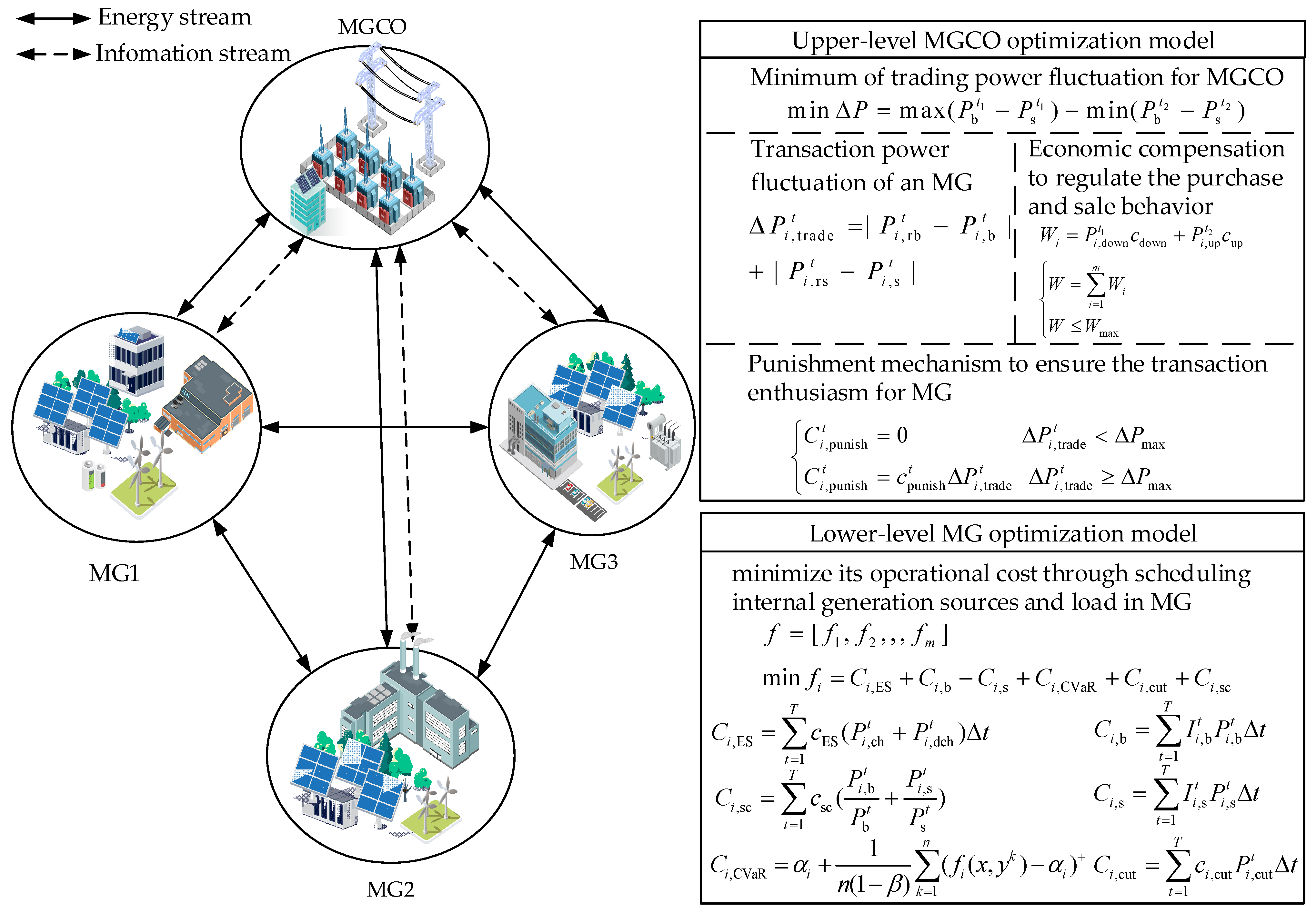
2. Trading Framework of Microgrid Cluster

2.1. Optimization Framework of Microgrid Cluster

The schematic diagram for system architecture of a microgrid cluster is illustrated in Figure 1 and consists of three microgrids and a microgrid cluster operator (MGCO). Each MG is equipped with an energy storage system (ESS), a wind turbine (WT), and photovoltaic (PV) load. Every MG is equipped with an independent energy management system, which is responsible for managing the economic operation of energy storage, new energy, and load within the microgrid. It can report power demand information to the MGCO and achieve information exchange with the MGCO. The MGs are also connected to the distribution grid which means that they have the option to engage in transactions with the distribution grid when the intracluster electricity price is unreasonable. The modeling formula on the right side of Figure 1 illustrates the optimization model of the upper layer MGCO and lower layer MG; the MGCO uses the minimum trading power fluctuation in the cluster as the objective function, and the MG uses the minimum operating cost as the objective function. The MGCO serves as the energy trading center, responsible for determining the intraelectricity price based on the transaction agreements. MGCO introduces penalty mechanisms related to trading volume fluctuations to ensure that each microgrid reports electricity consumption as accurately as possible. The lower-layer MG uses CVaR to quantify uncertainty to achieve reasonable energy dispatch and achieve economic operation.

2.2. Internal Pricing Mechanism of Microgrid Cluster

As the energy trading center, the MGCO in the upper layer has the authority to supervise and set prices. Through internal pricing mechanisms and supervision mechanisms, the MGCO coordinates the generation and consumption characteristics of each MG to enhance the overall benefits of the microgrid cluster. To encourage MG participation in intracluster transactions, the purchasing price set by the MGCO should be higher than the grid electricity purchase price, while the selling price should be lower than the grid electricity selling price.

Referring to the internal pricing criterion and the principles of transaction volume between microgrids in references [21,22], this paper proposes a new internal pricing mechanism. In this mechanism, if the surplus electricity of the MGC is less than the deficit electricity, the internal electricity price can be expressed as follows:

$$\left\{\begin{array}{l}{I}_{i,s}^t=\frac{c_s^t+c_b^t}{2}\\ I_{i,b}^t=\frac{P_{i,b}^t{P}_s^t(c_s^t-1)+2c_b^t{P}_b^t{P}_{i,b}^t}{2{(P_b^t)}^2}\end{array}\right.$$

(1)

where $P_b^t$ and $P_s^t$ represent the total purchasing power and total selling power in the microgrid cluster at the $t$th period, respectively. $P_{i,b}^t$ and $P_{i,s}^t$ denote the purchasing power and selling power of the microgrid at the $t$th period, respectively. $c_b^t$ and $c_s^t$ are, respectively, the selling price and grid feed-in price within the time period. $I_{i,b}^t$ and $I_{i,s}^t$ represent the internal purchasing price and selling price for the MG participating in intracluster transactions within the $t$th period, respectively.

When the surplus electricity is greater than the deficit electricity, the intracluster purchasing and selling electricity prices satisfy the following condition:

$$\left\{\begin{array}{l}{I}_{i,b}^t=\frac{c_s^t+c_b^t}{2}\\ I_{i,b}^t=\frac{P_{i,s}^t{P}_b^t(c_b^t-1)+2c_s^t{P}_s^t{P}_{i,s}^t}{2{(P_b^t)}^2}\end{array}\right.$$

(2)

The derivation process of intracluster transaction electricity prices is detailed in Appendix A.

2.3. Demand Response Model of Microgrid Cluster

As the energy trading center, the MGCO not only has the rights of pricing and supervision but also needs to assume certain social responsibilities. It aims to reduce the peak-to-valley difference in the trading power of the microgrid cluster through price incentive mechanisms. This can be achieved by satisfying the following condition:

$$\min \Delta P=\max (P_b^{t_1}-P_s^{t_1})-min(P_b^{t_2}-P_s^{t_2})$$

(3)

where $\Delta P$ represents the peak-to-valley difference in the trading power of the microgrid cluster, $t_1$ and $t_2$ are, respectively, the peak and valley time periods of the trading power of the microgrid cluster, $\max (P_b^{t_1}-P_s^{t_1})$ represents the peak trading power of the microgrid cluster, and $min(P_b^{t_2}-P_s^{t_2})$ denotes the valley trading power of the microgrid cluster.

To reduce the overall power fluctuation of the microgrid cluster, economic compensation is provided to MGs that reduce their purchasing demand and increase their selling demand during the peak trading power period, denoted as t₁. Conversely, economic compensation is provided to MGs that reduce their selling demand and increase their purchasing demand during the valley trading power period, denoted as t₂. This can be expressed as follows:

$$W_i=P_{i,down}^{t_1}{c}_{down}+P_{i,up}^{t_2}{c}_{up}$$

(4)

where $W_i$ represents the compensation cost for the ith MG. $P_{i,down}^{t_1}$ and $P_{i,up}^{t_2}$ denote the power reduction in time period t₁ and power increase in time period t₂, respectively. $c_{down}$ and $c_{up}$ represent the incentive prices for power reduction and power increase, respectively.

The total cost of compensating the demand response MGs should satisfy the following equation:

$$\left\{\begin{array}{l}W={\displaystyle \sum _{i=1}^m{W}_i}\\ W\le W_{\max }\end{array}\right.$$

(5)

where $W$ is the total compensation cost provided by the MGCO to MGs with the demand response, m is the number of MGs, and $W_{\max }$ is the upper limit of the compensation cost.

2.4. Punishment Mechanism of Microgrid Cluster

To avoid transactional chaos and default behavior, the penalty cost for MG default is calculated based on the difference between the reported and actual transaction volumes by MGCO. The setting of the penalty cost aims to ensure the enthusiasm for microgrid transactions while reducing MG default behavior. The specific principles are as follows:

(1)

Determining fluctuation range of the transaction power: Each MG reports its transaction power to the MGCO. The MGCO consolidates the reports and determines the power fluctuation range for the next trading day in the microgrid. The MGCO then provides each MG with the reference values of interactive power for each time period of the next trading day.

(2)

Determining power deviations: If the actual transaction power of an MG exceeds the previously determined transaction power fluctuation range, a penalty fee will be charged.

The calculation formula for the penalty fee satisfies the following equation:

$$\left\{\begin{array}{l}{C}_{i,punish}^t=0\hspace{1em}\hspace{1em}\hspace{1em}\hspace{1em}\hspace{1em}\Delta P_{i,trade}^t<\Delta P_{max}\\ C_{i,punish}^t=c_{punish}^t\Delta P_{i,trade}^t\hspace{1em}\Delta P_{i,trade}^t\ge \Delta P_{max}\end{array}\right.$$

(6)

where $C_{i,punish}^t$ represents the penalty cost imposed by the MGCO on the ith MG, $c_{punish}^t$ is the penalty price, $\Delta P_{i,trade}^t$ denotes the transaction power deviation, and $\Delta P_{max}$ represents the maximum fluctuation allowed in transaction power. $\Delta P_{i,trade}^t$ can be expressed as follows:

$$\Delta P_{i,trade}^t=|P_{i,rb}^t-P_{i,b}^t|+|P_{i,rs}^t-P_{i,s}^t|$$

(7)

where $P_{i,rb}^t$ represents the actual purchase power of the ith MG during the time t within a day, $P_{i,b}^t$ denotes the reported purchase power by the ith MG prior to the time t, $P_{i,rs}^t$ represents the actual sale power of the ith MG during the time t within a day, and $P_{i,s}^t$ denotes the reported sale power by the ith MG prior to the time t.

3. Uncertain Renewable Energy Generation Based on Scenario Reduction

The uncertainty of renewable energy in MG brings certain potential risks to its economic operation. In this paper, an uncertain model for renewable energy output is established based on the prediction deviation and probability distribution, aiming to achieve the prediction and scenario establishment of renewable energy.

3.1. Renewable Energy Output Model Considering Uncertainty

The prediction deviations of wind power and photovoltaic generation follow normal distribution [23], satisfying the following equation:

$$\left\{\begin{array}{l}{f}_{\Delta P_{i,WT}}(\Delta P_{i,WT}^t)=\frac{1}{\sqrt{2\mathsf{\pi }}{\sigma }_{i,WT}^t}{e}^{-{(\Delta P_{i,WT}^t)}^2/(2({\sigma }_{i,WT}^t{)}^2)}\\ f_{\Delta P_{i,PV}}(\Delta P_{i,PV}^t)=\frac{1}{\sqrt{2\mathsf{\pi }}{\sigma }_{i,PV}^t}{e}^{-{(\Delta P_{i,PV}^t)}^2/(2({\sigma }_{i,PV}^t{)}^2)}\end{array}\right.$$

(8)

where $\Delta P_{i,WT}^t$ and $\Delta P_{i,PV}^t$ represent the wind power prediction deviation and photovoltaic prediction deviation of the ith MG during time t, respectively. A negative prediction error indicates that the actual output is lower than the predicted output, while a positive prediction error indicates that the actual output is higher than the predicted output. ${\sigma }_{i,WT}^t$ and ${\sigma }_{i,PV}^t$ represent the forecasting standard deviations of wind power and photovoltaic in the ith MG during time t, respectively [24].

The prediction errors of power of WT and PV are independent. The joint distribution of these errors also follows a normal distribution:

$$f_{i,\Delta P_{i,SOD}}(\Delta P_{i,SOD}^t)=\frac{1}{\sqrt{2\mathsf{\pi }}{\sigma }_{i,SOD}^t}{e}^{-{(\Delta P_{i,SOD}^t)}^2/(2({\sigma }_{i,SOD}^t{)}^2)}$$

(9)

where

$$\left\{\begin{array}{l}\Delta P_{i,SOD}^t=\Delta P_{i,WT}^t+\Delta P_{i,PV}^t\\ {\sigma }_{i,SOD}^t=\sqrt{{({\sigma }_{i,WT}^t)}^2+{({\sigma }_{i,PV}^t)}^2}\end{array}\right.$$

(10)

where $\Delta P_{i,SOD}^t$ represents the system output deviation (SOD) of the ith MG during time t, and ${\sigma }_{i,SOD}^t$ denotes the standard deviation of the system output deviation of the ith MG during time t.

3.2. Scenario Analysis of Renewable Energy Generation

The basic approach for generating the wind and photovoltaic output scenario sets is as follows. First, the cumulative probability distribution data are obtained based on the prediction errors of the wind and PV output. Next, the Latin hypercube sampling (LHS) method is used to sample the data and generate a scenario set that includes scenarios of wind turbine and PV output. Finally, the scenario set is reduced using backward scenario reduction techniques to obtain n representative scenarios.

3.2.1. Generating Daily Wind Turbine and PV Power Scenarios Based on LHS

LHS is a stratified and dimension-wise random sampling method that allows us to obtain tail values with fewer samples. Compared to Monte Carlo sampling methods, it offers better sampling accuracy and efficiency [25].

In this paper, LHS is used to collect the prediction error of renewable energy power output. Firstly, based on the probability distribution of prediction errors, each error variable is divided into equally probable intervals. Random selection of prediction error values is made from each interval, and then the prediction values and error values are summed to generate scenarios of renewable energy output. The steps of LHS are as follows:

(1)

Establish a normal distribution model for the prediction error of renewable energy power;

(2)

Divide it into N equally probable intervals;

(3)

Randomly select sample values from each interval, where the cumulative probability of interval k is calculated as follows:

$$p_k=\frac{1}{N}{l}_u+\frac{k-1}{N}$$

(11)

where $l_u$ is a random number following a uniform distribution in the range [0, 1];

(4)

Assuming the inverse function of the prediction error distribution is $F^{-1}$, substitute $p_k$ into $F^{-1}$ to compute the sampled value $x_k$:

$$x_k=F^{-1}(p_k);$$

(12)

(5)

Calculate the sum of the renewable energy output prediction value $p_x$ and the sampling error value $x_k$ to obtain the scenario value $s_k$:

$$s_k=p_x+x_k.$$

(13)

3.2.2. Scenario Reduction

Due to the large number of renewable energy output scenarios generated using LHS, the time and computational complexity of model solving are increased. Therefore, it is necessary to employ suitable scenario reduction methods to reduce the number of scenarios while preserving the overall characteristics of the scenarios. Currently, commonly used reduction methods mainly utilize probabilistic distances such as Kolmogorov distance, Wasserstein distance, and Kantorovich distance. Kolmogorov distance is simple to compute but does not reflect tail characteristics well. Wasserstein distance performs better in capturing tail characteristics but has limited effectiveness for higher-order moments [26]. Kantorovich distance can overcome the aforementioned issues and better reflect the original probability distribution [27]. Thus, in this paper, a backward scenario reduction technique based on Kantorovich distance [28] is adopted to reduce scenarios to obtain the typical power output scenarios. The steps are as follows:

(1)

Initialization: Each renewable energy output scenario has an equal probability, i.e., the probability of each scenario is

$$p_k=\frac{1}{N};$$

(14)

(2)

Calculate the Kantorovich distance between any two scenarios:

$$D_k(s_m,s_v)=({\displaystyle \sum _{t=1}^T(}{L}_{m,t}-L_{v,t}){)}^{\frac{1}{2}};$$

(15)

(3)

Supposing the scenario with the minimum Kantorovich distance to scenario is $s_k$, calculate the product of its distance and probability:

$$P{D}_k(s_k,s_r)=D_k(s_k,s_r)p_r;$$

(16)

(4)

For each scenario, repeat steps (3), select the scenario $P{D}_k(s_k,s_r)$ with the minimum value as the scenario $d$, and delete this scenario. At this point, the number of scenarios becomes $N=N-1$, and the probability value of scenario $r$ is updated to

$$p_r=p_r+p_d;$$

(17)

(5)

Repeat steps (2) to (4) until the final reduced number of scenarios is $n$;

(6)

Obtain the typical scenarios of the renewable energy output.

4. Day-Ahead Optimization Model of Microgrid

The lower-layer optimization employs backward scenario reduction techniques to obtain multiple sets of typical scenarios for renewable energy generation. The CVaR theory is introduced to quantify the economic risks of transaction defaults and establish an optimization model with the objective of minimizing the comprehensive operating cost of the microgrid cluster.

4.1. MG Scheduling Based on CVaR

4.1.1. Objective Function

As an independent stakeholder, MG aims to minimize its operating cost through scheduling internal generation sources and load [29]. The objective function of MG is defined as follows:

$$f=[f_1,f_2,\dots ,f_m]$$

(18)

where $f$ represents the objective function of MG. The objective function of each MG satisfies the following:

$$\min f_i=C_{i,ES}+C_{i,b}-C_{i,s}+C_{i,CVaR}+C_{i,cut}+C_{i,sc}$$

(19)

where $C_{i,ES}$ denotes the operating and maintenance cost of energy storage in MG i, $C_{i,b}$ represents the purchasing cost of electricity for MG $i$, $C_{i,s}$ represents the revenue from selling electricity for MG $i$, $C_{i,CVaR}$ represents the potential economic losses for MG $i$, $C_{i,cut}$ represents the cost of load shedding for MG $i$, and $C_{i,sc}$ represents the service fee for participating in internal transactions within the cluster.

(1)

Operation and maintenance cost of energy storage

It is considered that the aging of the energy storage systems (ESSs) arises with their usage. The investment and construction cost of ESSs is converted to the unit cost of charging and discharging $c_{ES}$. The charging and discharging cost is given by

$$C_{i,ES}={\displaystyle \sum _{t=1}^T{c}_{ES}(P_{i,ch}^t+P_{i,dch}^t)\Delta t}$$

(20)

where $P_{i,ch}^t$ and $P_{i,dch}^t$ are, respectively, the charging and discharging power of the ESS for MG $i$ during the time t, $\Delta t$ represents the scheduling time interval, and $T$ represents the total number of scheduling cycles within the scheduling period.

(2)

Transaction cost

In order to balance the power of the MGC, electricity transactions are supervised by the MGCO, and the transaction cost is determined as follows:

$$\left\{\begin{array}{l}{C}_{i,s}={\displaystyle \sum _{t=1}^T{I}_{i,s}^t{P}_{i,s}^t\Delta t}\\ C_{i,b}={\displaystyle \sum _{t=1}^T{I}_{i,b}^t{P}_{i,b}^t\Delta t}\end{array}\right.$$

(21)

The service fee for MG’s participation in internal transactions within the cluster is given by

$$C_{i,sc}={\displaystyle \sum _{t=1}^T{c}_{sc}(\frac{P_{i,b}^t}{P_b^t}+\frac{P_{i,s}^t}{P_s^t})}$$

(22)

where $c_{sc}$ represents the unit service fee.

(3)

Load-shedding cost is

$$C_{i,cut}={\displaystyle \sum _{t=1}^T{c}_{i,cut}{P}_{i,cut}^t\Delta t}$$

(23)

where $c_{i,cut}$ represents the unit cost of load shedding.

4.1.2. Constraints

(1)

Energy storage constraints

The charging and discharging power of the energy storage device needs to satisfy

$$\left\{\begin{array}{l}0\le P_{i,ch}^t\le P_{i,ch,N}{s}_i^t\\ 0\le P_{i,dch}^t\le P_{i,dch,N}(1-s_i^t)\end{array}\right.$$

(24)

where $P_{i,ch,N}$ and $P_{i,dch,N}$ represent the maximum rated power for charging and discharging of the energy storage device. $s_i^t$ is a binary variable that restricts simultaneous charging and discharging of the energy storage. When $s_i^t$ is 0, the energy storage can discharge; otherwise, it can charge.

To avoid overcharging or overdischarging, which may affect the operating lifespan of the energy storage, the following constraint should be satisfied:

$$\left\{\begin{array}{l}{S}_{i,ES,\min }\le S_{i,ES}^t\le S_{i,ES,\max }\\ {\displaystyle \sum _{t=1}^{T_n}(P_{i,ch}^t+P_{i,dch}^t)\Delta t\le Q_{i,max}}\end{array}\right.$$

(25)

where $S_{i,ES,\max }$ and $S_{i,ES,\min }$ represent the maximum and minimum remaining capacities of the energy storage, respectively. $S_{i,ES}^t$ is the remaining capacity of the energy storage for MG i at time t. $Q_{i,max}$ is the upper limit of daily throughput for the energy storage of MG i, which is determined by factors such as the trading electricity price and energy storage losses.

To ensure continuous operation of the energy storage device, the remaining capacity at the beginning and end of the scheduling period should be equal, and the remaining capacity at time t should be

$$\left\{\begin{array}{l}{S}_{i,ES}^0=S_{i,ES}^T\\ S_{i,ES}^t=S_{i,ES}^{t-1}+P_{i,ch}^t{\eta }_{ch}\Delta t-\frac{P_{i,dch}^t}{{\eta }_{dch}}\Delta t\end{array}\right.$$

(26)

where $S_{i,ES}^0$ and $S_{i,ES}^T$ represent the remaining capacity of energy storage devices at the beginning and end of the scheduling period, respectively, and ${\eta }_{ch}$ and ${\eta }_{dch}$ represent the transmission efficiency of energy storage during charging and discharging, respectively.

(2)

Load constraints

The load consists of base load, shiftable load, and interruptible load, which satisfy

$$P_{i,load}^t=P_{i,trans}^t+P_{i,cut}^t+P_{i,bas}^t$$

(27)

where $P_{i,load}^t$ is the total load power of MG $i$ in time $t$, $P_{i,trans}^t$ is the power of shiftable load, $P_{i,cut}^t$ is the power of interruptible load, and $P_{i,bas}^t$ is the power of the base load.

For the shiftable load constraint, we have

$$\left\{\begin{array}{l}0\le P_{i,trans}^t\le P_{i,trans,max}{k}_{i,trans}^t\\ P_{i,trans}={\displaystyle \sum _{t=1}^T{P}_{i,trans}^t}\end{array}\right.$$

(28)

where $P_{i,trans,max}$ is the maximum load power of the shiftable load, $k_{i,trans}^t$ is a binary variable indicating whether the shiftable load is selected or not, and $P_{i,trans}$ is the total load amount of shiftable load during the entire scheduling period.

For the interruptible load constraint, it follows

$$0\le P_{i,cut}^t\le P_{i,cut,max}^t{k}_{i,cut}^t$$

(29)

where $P_{i,cut,max}^t$ is the maximum power that can be shed from the interruptible load of MG i at time t; $k_{i,cut}^t$ is a binary variable with a value of 1 when the interruptible load is shed, and 0 otherwise.

(3)

Transaction constraints

The power exchange between the MG and the external grid must satisfy the power limit on the interconnection line:

$$\left\{\begin{array}{l}0\le P_{i,b}^t\le P_{i,max}{k}_i^t\\ 0\le P_{i,s}^t\le P_{i,max}(1-k_i^t)\end{array}\right.$$

(30)

where $P_{i,max}$ is the power upper limit on the interconnection line of the MG $i$, and $k_i^t$ is a binary variable representing the power transaction mode. When $k_i^t$ is 1, the MG is purchasing electricity, and when it is 0, the MG is selling electricity.

(4)

Power balance constraint

The MG adjusts the charging and discharging power of energy storage and participates in intra-MG transactions to maintain power balance, given by

$$P_{i,dch}^t+P_{i,wt}^t+P_{i,pv}^t+P_{i,b}^t=P_{i,ch}^t+P_{i,load}^t+P_{i,s}^t$$

(31)

where $P_{i,wt}^t$ is the predicted power of wind turbines, $P_{i,pv}^t$ is the predicted power of photovoltaics, and $P_{i,\mathrm{load}}^t$ is the power load.

4.2. Economic Risk Model

In the day-ahead trading process, the uncertainty of wind turbine and PV power forecasts results in differences between the reported and actual traded volumes by the MG. The MG may face potential economic risks and penalties imposed by the MGCO due to excessive trading volume deviations. To ensure controllable risks, the CVaR theory is introduced to establish an economic risk quantification model.

CVaR theory, as a risk measurement theory in the financial field, is developed based on the value at risk (VaR) theory. It solves the problem of insufficient measurement of tail losses and the inability to examine the risk information below the quantile point in VaR theory. CVaR reflects the average value of potential risk losses exceeding the VaR value under a given confidence level. Currently, CVaR has been applied in risk decision making for power systems.

According to the definition, for a given confidence level $\beta \in (0,1)$, the VaR value can be obtained using the following formula:

$$\left\{\begin{array}{l}\psi (x,\alpha )={\displaystyle {\int }_{f(x,y)\le \alpha }\rho (y)\mathrm{d}y}\\ z_{\beta }(x)=\min \{\alpha \in R:\psi (x,\alpha )\ge \beta \}\end{array}\right.$$

(32)

where $f(x,y)$ represents the risk loss under decision variable $x$ and random variable $y$, $\rho (y)$ is the probability density function of random variable $y$, $\psi (x,\alpha )$ is the probability of loss not exceeding $\alpha$, and $z_{\beta }(x)$ is the VaR at confidence level $\beta$.

CVaR is the average value of losses exceeding the VaR value at confidence level $\beta$, and it satisfies

$$z_{CVaR}(x)=\frac{1}{1-\beta }{\displaystyle {\int }_{f(x,y)\ge z_{\beta }(x)}f(x,y)\rho (y)\mathrm{d}y}$$

(33)

where $z_{CVaR}(x)$ denotes the CVaR value under $\beta$.

Since the analytical expression of $z_{\beta }(x)$ is difficult to solve, an auxiliary variable is introduced to simplify the solution:

$$\left\{\begin{array}{l}{z}_{CVaR}(x)=\alpha +\frac{1}{1-\beta }{\displaystyle {\int }_{y\in R}{(f(x,y)-\alpha )}^{+}\rho (y)\mathrm{d}y}\\ {(f(x,y)-\alpha )}^{+}=\max \{f(x,y)-\alpha ,0\}\end{array}\right.$$

(34)

The integral term in Equation (34) is difficult to solve, and in practical applications, it is challenging to obtain the probability density function $\rho (y)$ of the random variable $y$. Therefore, $n$ sets of typical scenario data are generated through LHS and backward scenario reduction technique:

$$z(x)=\alpha +\frac{1}{n(1-\beta )}{\displaystyle \sum _{k=1}^n{(f(x,y^k)-\alpha )}^{+}}$$

(35)

where $z(x)$ is the estimated value of CVaR, and $y^k$ represents the set of $k$ typical scenario data.

As a result, the CVaR value for MG $i\mathrm{th}$ in Formula (19) can be expressed as follows:

$$C_{i,CVaR}={\alpha }_i+\frac{1}{n(1-\beta )}{\displaystyle \sum _{k=1}^n{(f_i(x,y^k)-{\alpha }_i)}^{+}}$$

(36)

where i represents the data of $i\mathrm{th}$ MG.

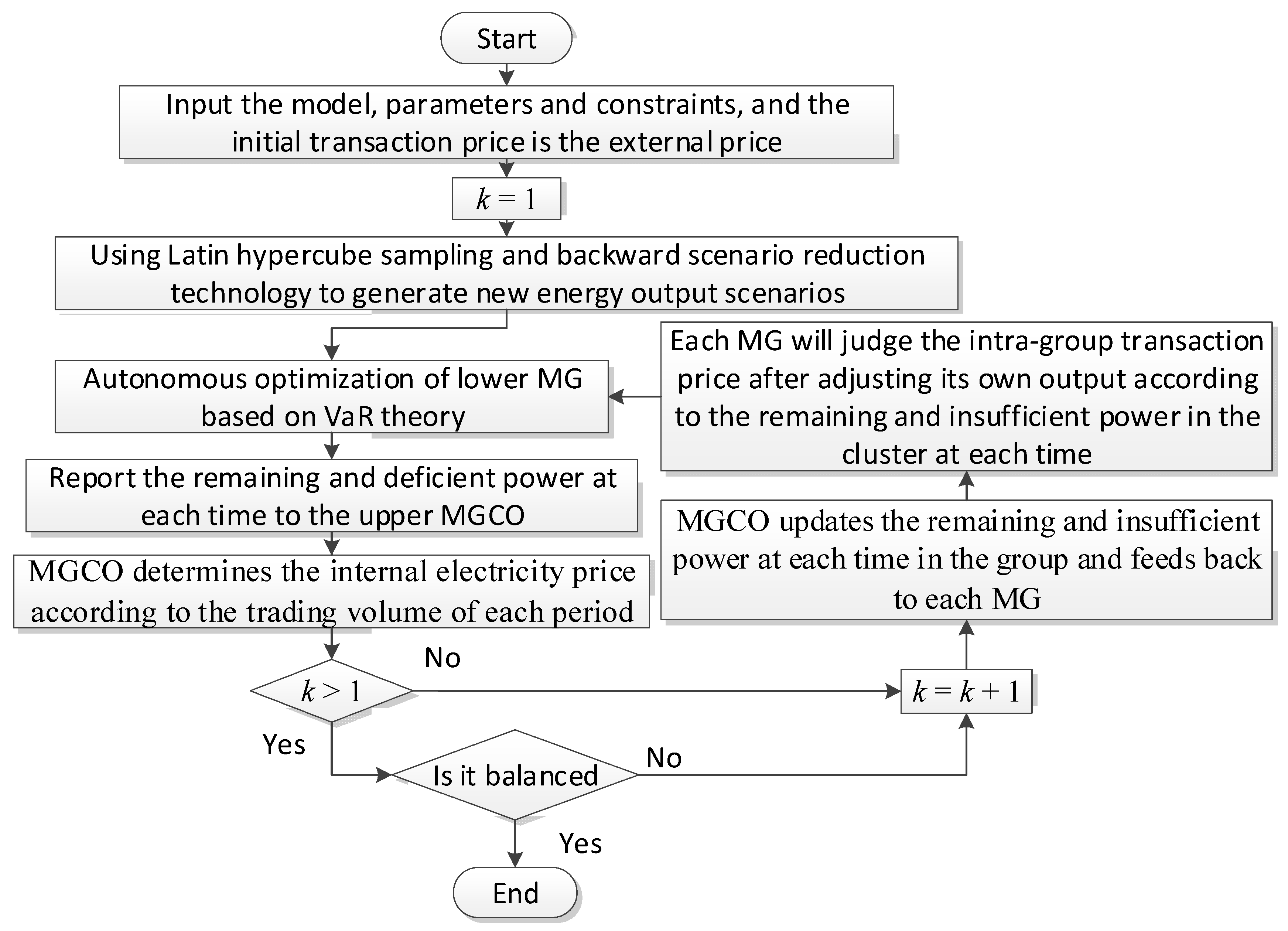
5. Solution Method for the Proposed Model

This paper adopts LHS to generate 100 sets of scenarios and utilizes a backward scenario reduction technique based on Kantorovich distance to reduce the number of scenarios, resulting in 10 typical scenarios [30,31]. Based on these scenarios, the economic risk is transformed into costs using CVaR theory. The optimization model is introduced, and the nonlinear constraints are linearized [32]. The MATLAB YALMIP toolbox (9.4.0.813654 (R2018a), https://yalmip.github.io/, accessed on 8 October 2023) is used to call CPLEX (https://www.ibm.com/products/ilog-cplex-optimization-studio, accessed on 8 October 2023) for solving. The scheduling time interval is 1 h, and there are three MGs. The flowchart of the solution process is shown in Figure 2. The specific steps are as follows:

• Step 1: Generate 100 sets of scenarios using LHS based on the normal distribution.
• Step 2: Reduce the number of scenarios using backward scenario reduction technique to obtain 10 typical scenarios.
• Step 3: Based on the electricity price of the distribution network, conduct autonomous optimization of each MG using CVaR theory to determine the operating states and trading volumes in each time period. Report the trading volumes to the MGCO.
• Step 4: The MGCO determines the internal electricity price based on the reported trading volumes and provides feedback to the MGs regarding the electricity purchase and sale demands in each time period.
• Step 5: Considering the supply and demand relationship within the group and the impact of adjusting their own trading volumes on the internal electricity price, the MGs dynamically adjust their operating states and trading volumes in each time period.
• Step 6: Repeat steps 4 and 5 until equilibrium is reached.
• Step 7: The solution is obtained.

6. Simulation Results

6.1. Parameters Setting

This paper analyzes the intra-MG trading strategies of an MG cluster consisting of three industrial park MGs and MGCO. Each of the three MGs is equipped with energy storage, PV generation systems, and small wind turbine turbines. The basic parameter information for these devices is shown in

Table 1. Parameters of the devices used in an MG.

Device	Parmeter	MG1	MG2	MG3
ESS	Max capacity (kWh)	285	240	200
	Min residual capacity (kW/h)	40	30	20
	Max charging power (kW)	50	25	20
	Min charging power (kW)	50	25	20
	Unit operation and maintenance costs (USD/kWh)	0.0415	0.0415	0.0415
Transferable load power	Minimum (kW)	0.5	0.5	0.5
	Maximum (kW)	3	3	3
	Total (kW)	10	15	20
Interruptible load power	Maximum (kW)	5	5	5
	Unit compensation expense (USD)	1.3793	1.3793	1.3793
Contact line	Maximum permitted power (kW)	80	70	60
MGCO	Service cost (USD/kWh)	0.0021	0.0021	0.0021

. The time-of-use electricity prices and grid electricity prices for the distribution network are presented in

Table 2. The time-of-use pricing and feed-in tariff for the grid.

	Time-of-Use Price (USD/kWh)	On-Grid Price (USD/kWh)	Periods
Peak	0.1712	0.1241	9:00–12:00; 16:00–20:00
Valley	0.1075	0.0690	8:00–9:00; 12:00–16:00; 20:00–23:00
Flat	0.0673	0.0415	00:00–8:00; 23:00–24:00

. The load power and output scenarios for wind turbines and PV are illustrated in Figure 3.

6.2. Simulation Results Analysis

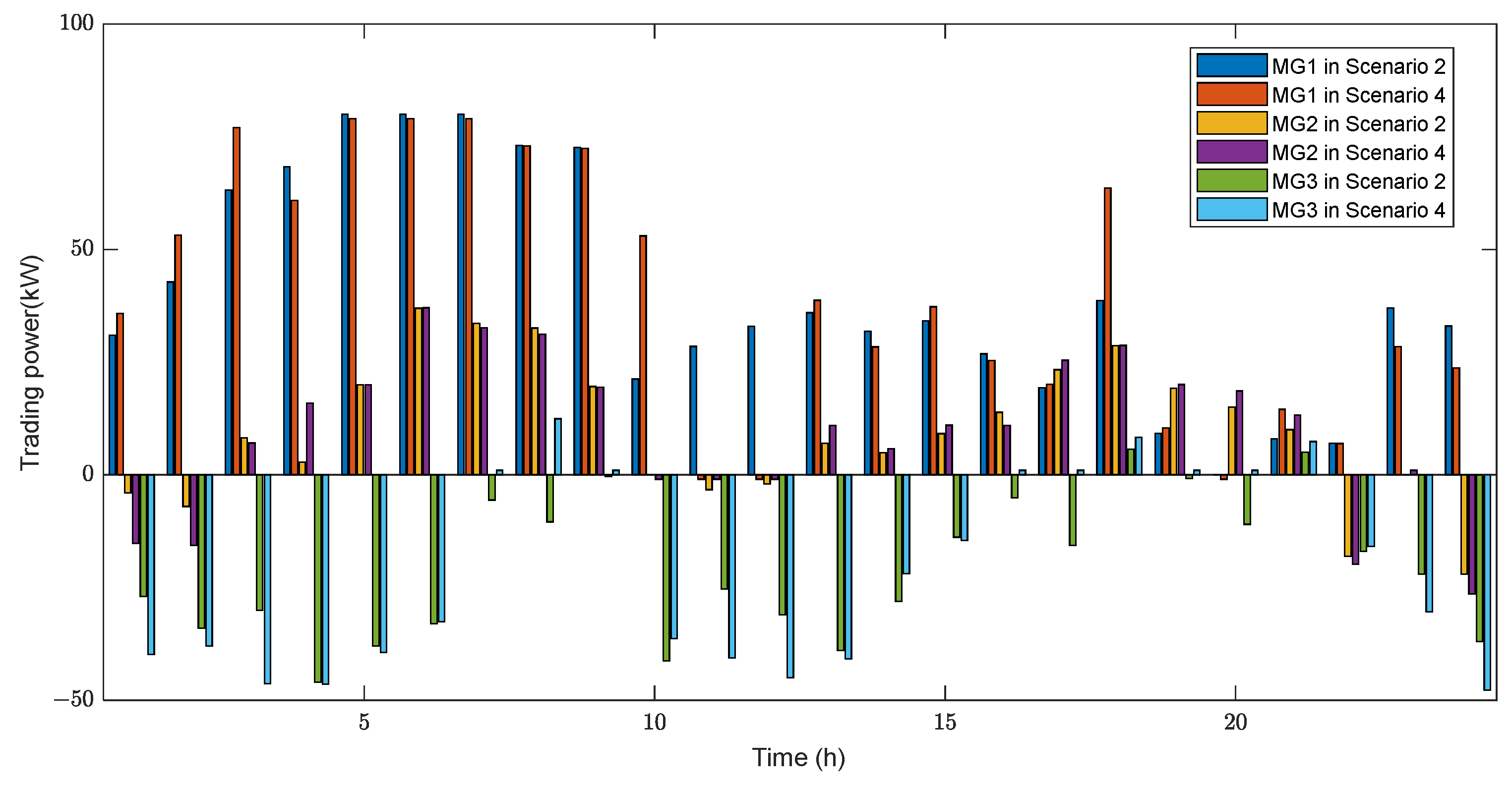
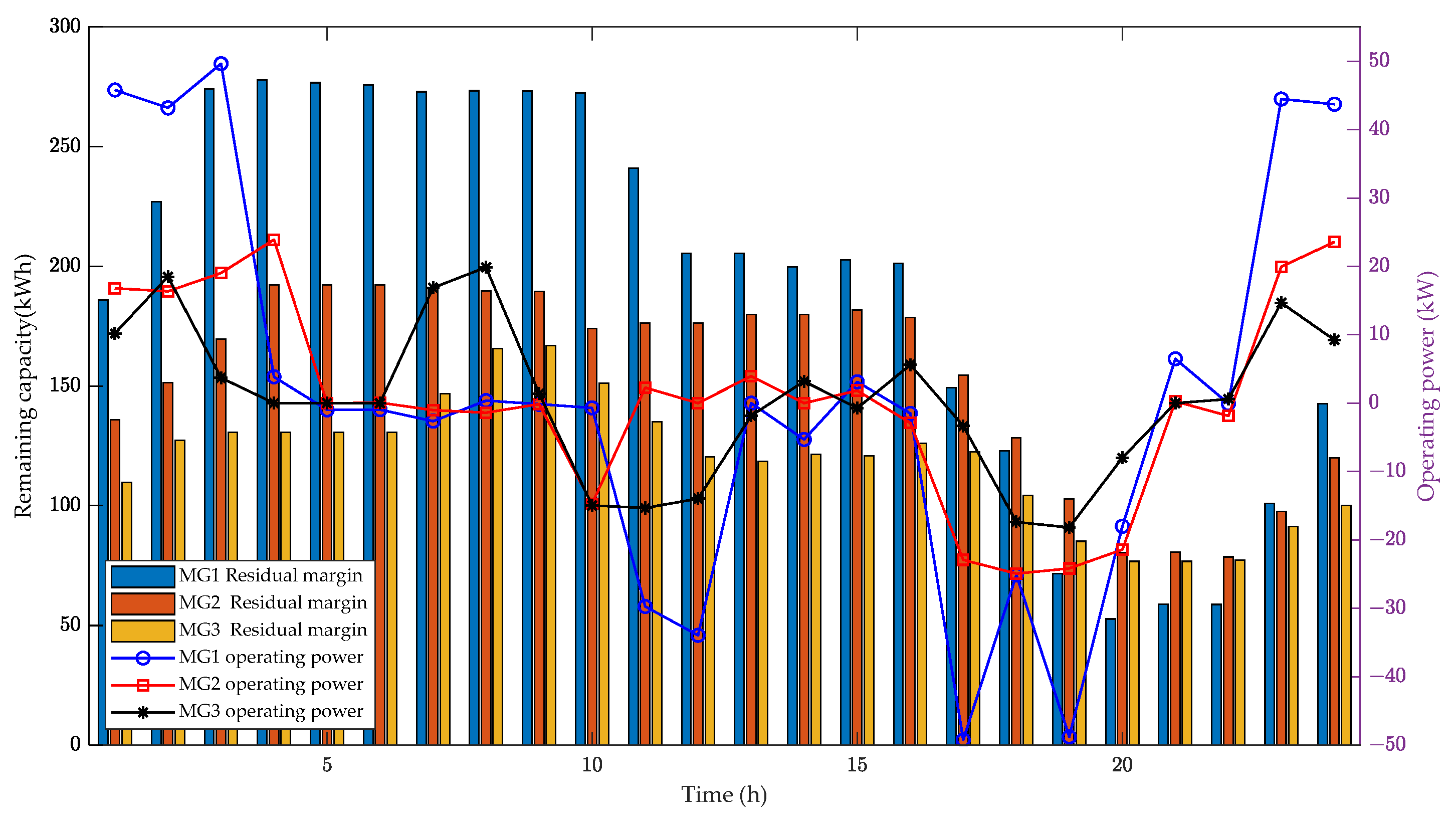
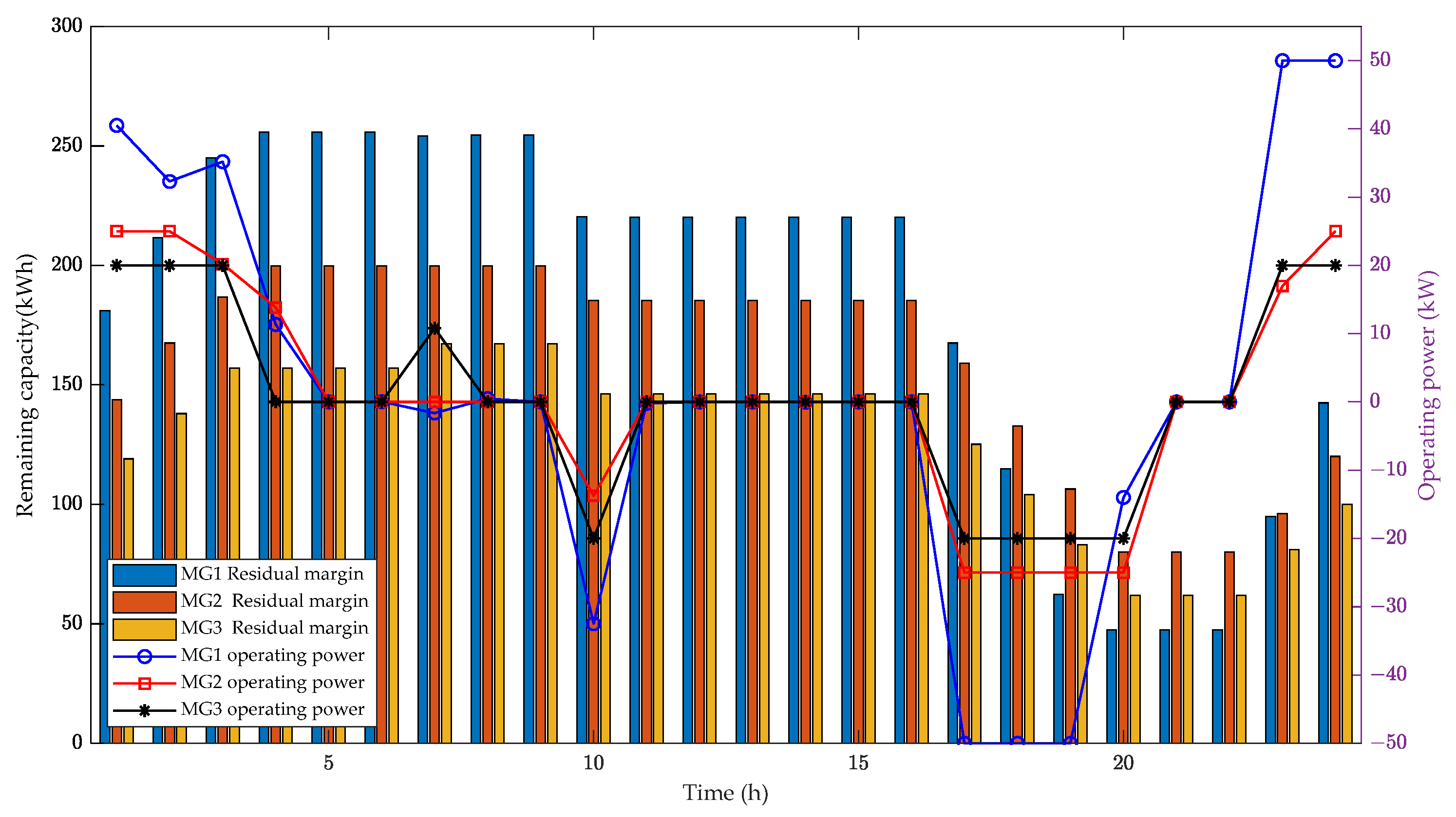
6.2.1. The Effect of Pricing Mechanism Considering Economic Risk and Demand Response on Transaction of MGs

The pricing mechanism considering economic risk quantification and demand response has an impact on the operation of MGs. To further investigate the operating conditions of each MG under different scenarios, this paper sets up four contrasting scenarios: scenario 1: MGs trading without considering demand response and economic risk quantification; scenario 2: MGs trading considering demand response but not economic risk quantification; scenario 3: MGs trading considering economic risk quantification but not demand response; scenario 4: MGs trading considering both demand response and economic risk quantification. By optimizing and solving each scenario using MATLAB, the operating results of each MG under different scenarios are obtained, as shown in

Table 3. Optimization results under different scenarios.

Scenarios	MG	Energy Storage Cost (USD)	Electricity Purchasing Cost (USD)	Electricity Sale Income (USD)	Load Shedding Cost (USD)	Compensation Fee (USD)	Service Cost (USD)	CvaR Value (USD)	Operation Cost (USD)
1	1	17.1462	83.5697	0	0	0	0.7034	15.5517	101.4193
	2	9.9228	31.2552	4.9876	0	0	0.1655	9.4966	36.3559
	3	4.5821	1.5076	37.4041	0	0	0.7669	13.6041	−30.5476
	Total	31.651	116.3324	42.3917	0	0	1.6359	38.6524	107.2276
2	1	17.3048	82.4276	0	0	1.869	0.891	16.5628	98.7545
	2	9.9228	30.7945	3.7614	0	0.5517	0.1972	8.229	36.6014
	3	8.7228	1.5076	39.6248	0	0.6345	0.9545	19.4524	−29.0745
	Total	35.9503	114.7297	43.3862	0	3.0552	2.0428	44.2441	106.2814
3	1	17.2386	84.8455	0.3434	0	0	1.9876	3.7752	103.7283
	2	9.8828	33.6883	5.8566	0	0	0.8717	2.3407	38.5862
	3	7.2303	2.9034	40.7338	0.9986	0	1.1338	3.211	−28.4676
	Total	34.3517	121.4372	46.9338	0.9986	0	3.9931	9.3269	113.8469
4	1	18.9434	84.0828	0.3959	0	0.9807	1.9917	4.0759	103.6414
	2	10.0786	32.5738	4.6469	0	0.5959	0.8055	2.1766	38.2152
	3	8.1766	3.8428	41.7834	0.0566	0.2883	1.1793	3.2331	−28.8166
	Total	37.1986	120.4993	46.8262	0.0566	1.8648	3.9766	9.4855	113.04

.

Comparing scenarios 1 and 2, it can be observed that in scenario 2, the operating cost of MG1 decreases by USD 2.6648, while the operating costs of MG2 and MG3 increase by USD 0.2455 and USD 1.4731, respectively. The total operating cost of the MGs decreases by USD 0.9462. This indicates that MGs with a large demand for electricity can better achieve demand response in MGs and thus obtain greater benefits. The decrease in total operating cost is due to the fact that when considering the demand response mechanism, MGs can optimize the operating cost further by adjusting energy storage output and mobilizing flexible loads, thus reducing the overall cost. In scenario 2, the CVaR values of MG1 and MG3 increase by USD 1.0110 and USD 5.8483, respectively, while the CVaR value of MG2 decreases by USD 1.2676. The total CvaR value increases by USD 5.5917. The increase in the total CVaR value of MGs is because economic risk is not converted into costs in scenario 2 and only the objective of minimizing operating costs is considered, resulting in an increase in the total CVaR value. Furthermore, both scenario 1 and scenario 2 do not consider the conversion of economic risk into costs in the trading model, leading to excessively high CVaR values in both scenarios.

In conclusion, comparing scenarios 3 and 4 reveals that in scenario 4, the operating costs of each MG decreased by USD 0.0869, USD 0.371, and USD 0.349, respectively. At the same time, the CVaR values of MG1 and MG3 increased by USD 0.3007 and USD 0.0221, while the CVaR value of MG4 decreased by USD 0.1641. The overall operating costs of the microgrid cluster decreased by USD 0.8069, while the CVaR value increased by USD 0.1586. Therefore, the operating scheme in scenario 4 is favorable for the overall operation of the microgrid cluster. This is attributed to the demand response in scenario 4, which enables MGs to obtain better transaction information within the microgrid cluster, resulting in more favorable transaction adjustments. As a result, the operating costs and potential economic risk losses are reduced, ensuring the safe and economic operation of the microgrid cluster.

The comparison of transaction volumes in each time period between scenarios 2 and 4 is illustrated in Figure 4.

According to Figure 4, positive transaction values represent the purchased electricity quantity of MGs, while negative values represent the sold electricity quantity. It can be observed that in both scenarios, MG1 has a significant demand for purchased electricity. To mitigate economic risk losses, MG1 shows varying degrees of increased purchased electricity quantity during time periods 1–3, 9, 13, 15, and 18. Under scenario 4, MG1 and MG2 exhibit a slight increase in purchased electricity demand, as indicated by the data in Table 3, with corresponding increases in energy storage operation costs of USD 1.6386 and USD 0.1559, respectively. In both scenarios, MG3 has a high demand for selling electricity. Under scenario 4, where risk costs are incorporated into the transaction model, the sold electricity quantity during time periods 11–13 increases by 31.15 kWh. This increase is advantageous for MG3’s economic gains as it corresponds to peak electricity price periods.

The operating statuses of energy storage devices in scenarios 2 and 4 are depicted in Figure 5 and Figure 6, respectively.

The positive values of charging and discharging power in Figure 5 and Figure 6 represent energy storage charging, while the negative values represent energy storage discharging. A comparison reveals that in scenario 4, compared to scenario 2, the total throughput power and total throughput quantity of energy storage increase for MG1 and MG2. The increase in total throughput quantity is attributed to scenario 4 incorporating risk costs into the transaction model, leading to the need for energy storage to store more energy to mitigate economic risks associated with uncertain renewable energy generation. The decrease in total throughput quantity for MG3 is due to its smaller load power demand and greater demand for selling electricity. To address the uncertainty of renewable energy generation, MG3 requires a larger energy storage capacity to accommodate surplus energy when the actual renewable energy generation exceeds the predicted values. This helps to reduce default penalty costs.

The overall peak-to-valley difference of the microgrid under different trading scenarios is presented in

Table 4. Peak-to-valley difference in different scenarios.

Scenario	Peak-Vally Difference (kW)
1	168.77
2	151.34
3	177.56
4	166.98

.

By comparing the data in Table 4, it can be observed that scenario 3 has the largest peak-to-valley difference. This is because in this scenario, only the potential economic risks associated with MG operations are considered, without the participation of demand response to reduce the peak-to-valley difference. Consequently, this scenario exhibits the highest peak-to-valley difference. On the other hand, scenario 2 has the smallest peak-to-valley difference as it only considers the participation of demand response without accounting for potential economic risks, resulting in the smallest peak-to-valley difference in energy transactions within the microgrid. In scenario 4, the peak-to-valley difference in energy transactions within the microgrid is relatively small. Combining this observation with the information in Table 3, it can be inferred that the trading strategy in this scenario ensures effective reduction of the peak-to-valley difference in energy transactions within the microgrid at a lower level of potential economic risks.

6.2.2. The Influence of Confidence on Operation Results

Confidence level reflects the decision maker’s aversion to risk and their willingness to accept it. To verify the impact of different confidence levels on the overall operation of the microgrid cluster, a comparison of the cluster’s operation under different confidence levels was conducted, and the specific results are shown in

Table 5. Operating costs at different confidence levels.

Confidence Level	CVaR (USD)	Operation Cost (USD)	Total Cost (USD)
0.90	9.4855	113.04	122.5255
0.85	8.8262	111.9324	120.7586
0.80	7.6069	111.6703	119.2772
0.75	7.1490	111.1007	118.2497

.

As shown in Table 5, with an increase in the confidence level, the values of CVaR, operating costs, and total costs exhibit an overall upward trend. As the confidence level increases, in order to mitigate the economic risks associated with the uncertainty of renewable energy generation, energy storage devices need to reserve more energy to address the economic losses resulting from the uncertainty of renewable energy output.

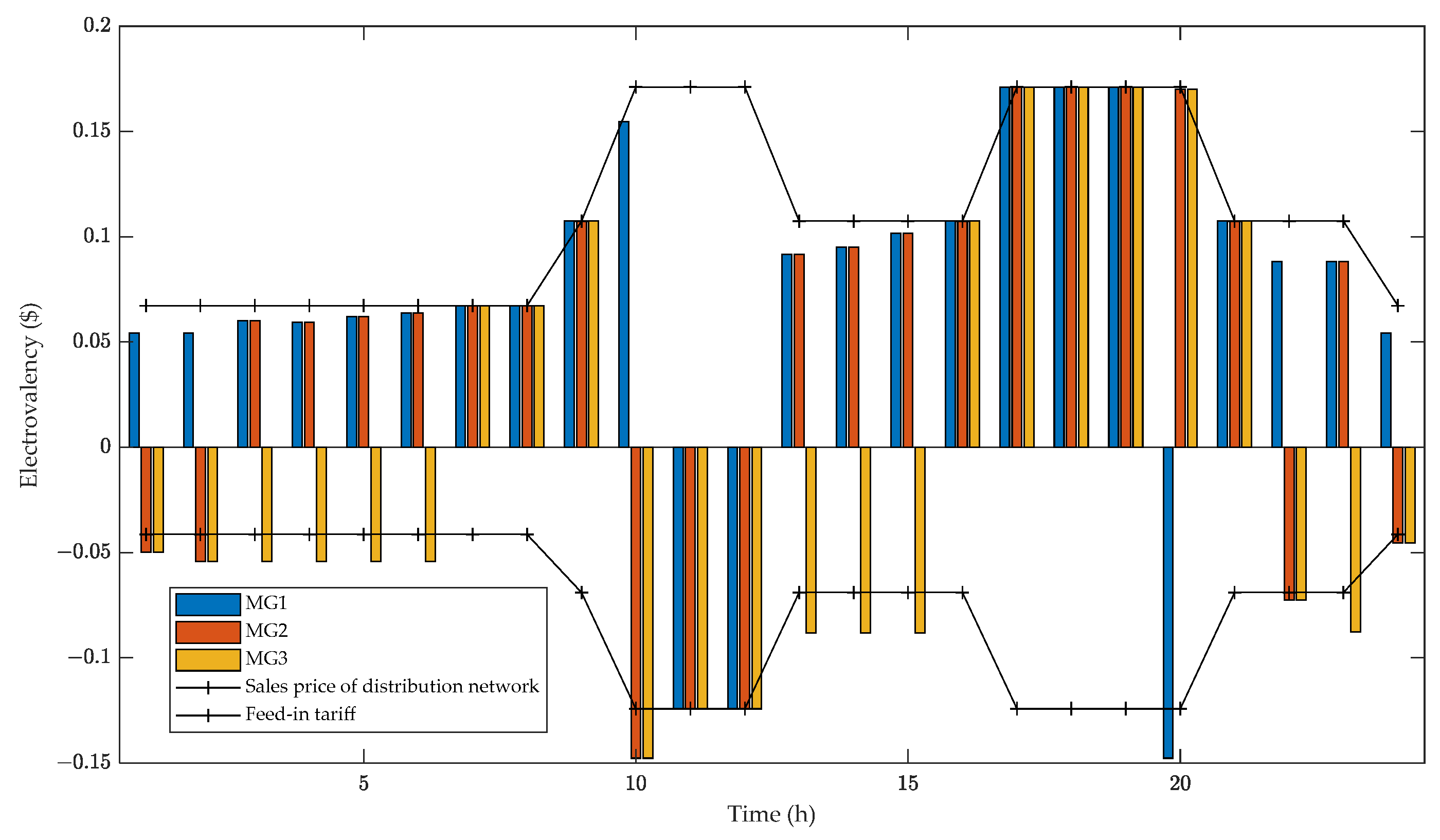
6.2.3. Rationality Analysis of Internal Price of MGs

To verify the reasonableness of the equilibrium electricity prices in each time period, an analysis is conducted, comparing the intracluster transaction prices with the distribution grid electricity prices in each time period.

In Figure 7, positive prices indicate the purchasing prices of MGs during the corresponding time periods, while negative prices indicate the selling price of MGs. From the figure, it can be observed that during time periods 7–9, 16–19, and 21, the transaction prices of all MGs are equal to the distribution grid time-of-use prices. This is because during these time periods, MGs have no selling demand. According to the pricing mechanism, in time periods where there is only selling demand or only purchasing demand, the internal transaction prices are equal to the distribution grid prices. For the remaining time periods, the purchasing prices of MGs are consistently lower than the distribution grid time-of-use prices, while the selling prices are higher than the grid selling prices. This encourages the participation of MGs in intracluster transactions. These results confirm the rationality and effectiveness of the intracluster pricing mechanism.

7. Conclusions

In this study, the problem of how to address the quantification of economic risks caused by the uncertainty of renewable energy generation in microgrid cluster transactions is evaluated. A two-layer power trading model is proposed based on intracluster demand response and CVaR risk quantification. Through case analysis on electricity trading in microgrid clusters under different scenarios, the following conclusions are drawn:

(1)

By quantifying the uncertain economic risks as risk costs using CVaR theory and incorporating them into the microgrid cluster trading model, although it increases the operating costs for each MG, it effectively reduced the system’s economic risk losses. Combined with demand response mechanisms and the regulation of flexible resources, the strategy proposed in this paper can reduce the overall operating costs of the MG, and decrease peak-to-valley differences in the microgrid cluster.

(2)

The analysis of the influence of different confidence levels on the operating costs of the microgrid cluster reveals that as the confidence level increases from 75% to 90%, both the operating costs and economic risk losses of the system increase by about 1.75% and 3.62%.

(3)

Through a comparative analysis of intracluster electricity prices and distribution grid electricity prices, the pricing mechanism proposed can effectively adjust the purchasing price for MGs and increase the selling price, and it is useful to incentivize MGs to actively participate in microgrid cluster transactions.

This study did not consider the impact of the weight between operating costs and risk costs on the results of the system’s power transactions. Future research can further explore related studies to develop more comprehensive power trading mechanism and more reasonable risk quantification methods, thereby promoting the sustained and stable operation of microgrid clusters.

References

1. Wei, Y.M.; Chen, K.; Kang, J.N.; Chen, W.; Wang, X.Y.; Zhang, X. Policy and Management of Carbon Peaking and Carbon Neutrality: A Literature Review. Engineering 2022, 14, 52–63. [Google Scholar] [CrossRef]
2. United Nations Economic and Social Council. From Global to Local: Supporting Sustainable and Resilient Societies in Urban and Rural Communities. 2018. Available online: https://www.un.org/ecosoc/zh/events/2018/ecosoc-high-level-segment-global-local-supporting-sustainable-and-resilient-societies (accessed on 17 April 2023).
3. Erdiwansyah; Mahidin; Husin, H.; Nasaruddin; Zaki, M.; Muhibbuddin. A critical review of the integration of renewable energy sources with various technologies. Prot. Control Mod. Power Syst. 2021, 6, 3. [Google Scholar] [CrossRef]
4. Mohler, D.; Sowder, D. Chapter 23—Energy storage and the need for flexibility on the grid. In Renewable Energy Integration; Jones, L.E., Ed.; Academic Press: Boston, MA, USA, 2014; pp. 285–292. [Google Scholar]
5. Zenginis, I.; Vardakas, J.S.; Echave, C.; Morató, M.; Abadal, J.; Verikoukis, C.V. Cooperation in microgrids through power exchange: An optimal sizing and operation approach. Appl. Energy. 2017, 203, 972–981. [Google Scholar] [CrossRef]
6. Arefifar, S.A.; Ordonez, M.; Mohamed, Y.A.R.I. Voltage and current controllability in multi-microgrid smart distribution systems. IEEE Trans Smart Grid. 2018, 9, 817–826. [Google Scholar] [CrossRef]
7. Li, Z.; Wu, L.; Xu, Y.; Wang, L.; Yang, N. Distributed tri-layer risk-averse stochastic game approach for energy trading among multi-energy microgrids. Appl. Energy 2023, 331, 120282. [Google Scholar] [CrossRef]
8. Wu, Q.; Xie, Z.; Ren, H.; Li, Q.; Yang, Y. Optimal trading strategies for multi-energy microgrid cluster considering demand response under different trading modes: A comparison study. Energy 2022, 254, 124448. [Google Scholar] [CrossRef]
9. Hou, J.; Yu, W.; Xu, Z.; Ge, Q.; Li, Z.; Meng, Y. Multi-time scale optimization scheduling of microgrid considering source and load uncertainty. Electr. Power Syst. Res. 2023, 216, 109037. [Google Scholar] [CrossRef]
10. Liu, N.; Yu, X.; Wang, C.; Li, C.; Ma, L.; Lei, J. Energy-Sharing Model with Price-Based Demand Response for Microgrids of Peer-to-Peer Prosumers. IEEE Trans Power Syst. 2017, 32, 3569–3583. [Google Scholar] [CrossRef]
11. Daneshvar, M.; Mohammadi-Ivatloo, B.; Asadi, S.; Anvari-Moghaddam, A.; Rasouli, M.; Abapour, M.; Gharehpetian, G.B. Chance-constrained models for transactive energy management of interconnected microgrid cluster. J. Clean. Prod. 2020, 271, 122177. [Google Scholar] [CrossRef]
12. Beltran-Royo, C. Fast scenario reduction by conditional scenarios in two-stage stochastic MILP problems. Optim. Methods Softw. 2019, 37, 23–44. [Google Scholar] [CrossRef]
13. Alabdulwahab, A.; Abusorrah, A.; Zhang, X.; Shahidehpour, M. Coordination of Interdependent Natural Gas and Electricity Infrastructures for Firming the Variability of Wind Energy in Stochastic Day-Ahead Scheduling. IEEE Trans. Sustain. Energy 2015, 6, 606–615. [Google Scholar] [CrossRef]
14. Li, Z.; Xu, Y.; Wang, P.; Xiao, G. Restoration of Multi-Energy Distribution Systems with Joint District Network Reconfiguration by A Distributed Stochastic Programming Approach. IEEE Trans. Smart Grid 2023, 1. [Google Scholar] [CrossRef]
15. Das, S.; Basu, M. Day-ahead optimal bidding strategy of microgrid with demand response program considering uncertainties and outages of renewable energy resources. Energy 2020, 190, 116441. [Google Scholar] [CrossRef]
16. Cheng, J.; Yan, Z.; Wang, H.; Xu, X. A Risk-Controllable Day-Ahead Transmission Schedule of Surplus Wind Power with Uncertainty in Sending Grids. Int. J. Electr. Power Energy Syst. 2022, 139, 107649. [Google Scholar] [CrossRef]
17. Ju, X.; Liu, X.; Liu, S.; Xiao, Y. Optimal scheduling of wind-photovoltaic power-generation system based on a copula-based conditional value-at-risk model. Clean Energy 2022, 6, 550–556. [Google Scholar] [CrossRef]
18. Li, Z.; Wu, L.; Xu, Y. Risk-Averse Coordinated Operation of a Multi-Energy Microgrid Considering Voltage/Var Control and Thermal Flow: An Adaptive Stochastic Approach. IEEE Trans Smart Grid 2021, 12, 3914–3927. [Google Scholar] [CrossRef]
19. Ghasemi, A.; Jamshidi Monfared, H.; Loni, A.; Marzband, M. CVaR-based retail electricity pricing in day-ahead scheduling of microgrids. Energy 2021, 227, 120529. [Google Scholar] [CrossRef]
20. Zhang, N.; Sun, Q.; Yang, L. A two-stage multi-objective optimal scheduling in the integrated energy system with We-Energy modeling. Energy 2021, 215, 119121. [Google Scholar] [CrossRef]
21. Lin, Z.D.; Zhao, B.; Li, C.Y.; Wang, X.J.; Ni, C.W.; Zhang, H.Y. Economic dispatch of multi-microgrid considering false information based on system of systems architecture. Autom. Electr. Power Syst. 2020, 44, 37–44. [Google Scholar]
22. Kim, H.J.; Chung, Y.S.; Kim, S.J.; Kim, H.T.; Jin, Y.G.; Yoon, Y.T. Pricing mechanisms for peer-to-peer energy trading: Towards an integrated understanding of energy and network service pricing mechanisms. Renew. Sustain. Energy Rev. 2023, 183, 113435. [Google Scholar] [CrossRef]
23. Qi, B.; Chen, J.; Zhao, Y.; Jiao, P. Expectation-maximisation model for stochastic distribution network planning considering network loss and voltage deviation. IET Gener. Transm. Distrib. 2019, 13, 248–257. [Google Scholar] [CrossRef]
24. Liu, J.; Chen, J.; Yan, G.; Chen, W.; Xu, B. Clustering and dynamic recognition based auto-reservoir neural network: A wait-and-see approach for short-term park power load forecasting. iScience 2023, 26, 107456. [Google Scholar] [CrossRef] [PubMed]
25. Qu, Z.L.; Chen, J.J.; Peng, K.; Zhao, Y.L.; Rong, Z.K.; Zhang, M.Y. Enhancing stochastic multi-microgrid operational flexibility with mobile energy storage system and power transaction. Sustain. Cities Soc. 2021, 71, 102962. [Google Scholar] [CrossRef]
26. Hochreiter, R.; Pflug, G.C. Financial scenario generation for stochastic multi-stage decision processes as facility location problems. Ann. Oper. Res. 2007, 152, 257–272. [Google Scholar] [CrossRef]
27. Dupačová, J.; Gröwe-Kuska, N.; Römisch, W. Scenario reduction in stochastic programming an approach using probability metrics. Math. Program Ser. B. 2003, 95, 493–511. [Google Scholar] [CrossRef]
28. Shi, L.; Luo, Y.; Tu, G.Y. Bidding strategy of microgrid with consideration of uncertainty for participating in power market. Int. J. Electr. Power Energy Syst. 2014, 59, 1–13. [Google Scholar] [CrossRef]
29. Castellanos, J.; Correa-Flórez, C.A.; Garcés, A.; Ordóñez-Plata, G.; Uribe, C.A.; Patino, D. An energy management system model with power quality constraints for unbalanced multi-microgrids interacting in a local energy market. Appl. Energy 2023, 343, 121149. [Google Scholar] [CrossRef]
30. Kammammettu, S.; Li, Z. Scenario reduction and scenario tree generation for stochastic programming using Sinkhorn distance. Comput. Chem. Eng. 2023, 170, 108122. [Google Scholar] [CrossRef]
31. Zhang, T.; Liu, J.; Yang, X.; Huo, R.; Guo, Y.; Li, Y. Economic Dispatch of Microgrid Considering Active/Passive Demand Response and Conditional Value at Risk. High Volt. Eng. 2021, 47, 3292–3302. [Google Scholar]
32. Li, R.; Wei, W.; Mei, S.; Hu, Q.; Wu, Q. Participation of an Energy Hub in Electricity and Heat Distribution Markets: An MPEC Approach. IEEE Trans Smart Grid 2019, 10, 3641–3653. [Google Scholar] [CrossRef]
Figure 1. Schematic diagram for system architecture of a microgrid cluster.
Electronics 12 04327 g001
Figure 2. Flow chart of optimization.
Electronics 12 04327 g002
Figure 3. Typical scenarios of wind and solar power and distribution of load in an MG: (a) MG1; (b) MG2; (c) MG3.
Electronics 12 04327 g003aElectronics 12 04327 g003b
Figure 4. Comparison of trading quantity under scenarios 2 and 4.
Electronics 12 04327 g004
Figure 5. Operation status of energy storage in scenario 2.
Electronics 12 04327 g005
Figure 6. Operation status of energy storage in scenario 4.
Electronics 12 04327 g006
Figure 7. Comparison of the trading price of electricity within the cluster and the electricity price of the distribution network.
Electronics 12 04327 g007