A Lightweight Network Based on Improved YOLOv5s for Insulator Defect Detection

Abstract

Insulators on transmission lines can be damaged to different degrees due to extreme weather conditions, which threaten the safe operation of the power system. In order to detect damaged insulators in time and meet the needs of real-time detection, this paper proposes a multi-defect and lightweight detection algorithm for insulators based on the improved YOLOv5s. To reduce the network parameters, we have integrated the Ghost module and introduced C3Ghost as a replacement for the backbone network. This enhancement enables a more efficient detection model. Moreover, we have added a new detection layer specifically designed for small objects, and embedded an attention mechanism into the network, significantly improving its detection capability for smaller insulators. Furthermore, we use the K-means++ algorithm to recluster the prior boxes and replace Efficient IoU Loss as the new loss function, which has better matching and convergence on the insulator defect dataset we constructed. The experimental results demonstrate the effectiveness of our proposed algorithm. Compared to the original algorithm, our model reduces the number of parameters by 41.1%, while achieving an mAP@0.5 of 94.8%. It also achieves a processing speed of 32.52 frames per second. These improvements make the algorithm well-suited for practical insulator detection and enable its deployment in edge devices.

1. Introduction

As the electric power industry continues to grow, transmission lines are rapidly expanding across the country [1]. However, the prolonged exposure of electrical equipment to extreme weather conditions in natural environments can cause various degrees of damage. Insulators, in particular, are highly vulnerable to such damage. Due to the unique properties of insulators, transmission lines are equipped with insulators made of different materials, such as glass, ceramic, and composite. These insulators are susceptible to different types of faults, including breakage, string drop, self-explosion, and flashovers. Regular inspections are indispensable for identifying defective insulators, but manual inspections suffer from low efficiency and are challenging [2]. In this regard, the adoption of aerial drones equipped with deep learning algorithms has been proposed as an effective solution. Therefore, it is critically important to explore object detection networks capable of identifying multiple defects in insulators specifically.

The task of object detection in deep learning is a hot research topic nowadays [3], and the models of target detection can be roughly divided into two categories according to the stages of detection: one-stage models and two-stage models. The representative two-stage models include the Region-based Convolutional Neural Network (R-CNN) [4], Fast R-CNN [5] and Faster R-CNN [6], etc. In the field of object detection for insulators on transmission lines, a new Faster R-CNN algorithm has been proposed in the literature [7], which uses the ResNet-101 as the backbone network and introduces a new feature enhancement mechanism, thus achieving significant improvements in the detection accuracy and recall rate of the model. Moreover, in order to further enhance the detection accuracy of the model, the literature [8] takes into account the slender shape characteristics of most electrical devices and optimizes the aspect ratio of their anchor frames based on the Faster R-CNN algorithm. This optimization serves to better align the model with the specific characteristics of the objects being detected. Although the two-stage model has advantages in terms of accuracy, it has disadvantages in terms of model size and processing speed.

The Single Shot Detector (SSD) [9], RetinaNet [10], and You Only Look Once (YOLO) [11] algorithm series, as one-stage algorithms, eliminate the need for a Region Proposal Network (RPN). Instead, they generate the location coordinates and class probabilities of objects using a single detection object. This approach enables faster and more accurate detection capabilities. The literature [12] presents a lightweight SSD network that utilizes the mobilenets as the backbone network to replace the original network model, which effectively reduces redundant computations. In the literature [13], the YOLOv3 network is enhanced by incorporating a multi-scale feature fusion structure and multiple feature mapping modules. This modification aims to tackle the challenges posed by the complex background in aerial images and the presence of insulators with different sizes. By utilizing multi-scale features and integrating them through fusion, the network becomes more capable of accurately detecting insulators of varying sizes in aerial images where the background complexity can cause difficulties for detection algorithms. Furthermore, the EIoU loss function is applied to YOLOv3 in literature [14], which enhances the overlap between the predicted frame and the actual frame and leads to an accelerated speed of convergence. In the literature [15], the GhostNet module is utilized to reconstruct the backbone network of the YOLOv4 model. Additionally, deep separable convolution is employed in the feature fusion layer. These approaches contribute to promoting a lightweight architecture for the model. These studies have explored advanced techniques to improve the performance of object detection algorithms, which can be applied in the context of detecting damage to insulators in power transmission lines. However, more efforts need to be made to further validate and optimize these methods.

The YOLOv5 model represents an iterative optimization of the YOLOv4 [16] algorithm, inheriting some advantages from both YOLOv3 [17] and YOLOv4. Currently, this algorithm is among the most widely used in industry. This literature [18] proposes several methods to solve the problem of insulator masking, which can cause missed detections. The proposed approaches include introducing the EIoU concept in calculating regression loss, using the AFK-MC2 algorithm for training, and applying a clustering NMS algorithm for eliminating redundant bounding box predictions. These methods aim to improve the detection performance of insulators and minimize missed detections caused by masking. In the literature [19], the replacement of the original loss function with the focal loss function, combined with the incorporation of a dynamic weight assignment method, has yielded substantial improvements in both model accuracy and recall. Consequently, this approach has successfully facilitated the rapid detection of insulator defects. Lastly, the literature [20] proposes a detection network for a fuzzy insulator based on YOLOv5, which includes a channel attention mechanism to enhance the detection capability in foggy conditions. The above improvements and optimizations made for the YOLOv5 algorithm provide a reference for the research of the defect detection algorithm for insulators in this paper.

Detecting insulators on transmission lines requires lightweight models that can be deployed on edge devices. Thus, the key focus of research in this area is to minimize the number of model parameters while ensuring that accuracy is not compromised. Moreover, insulators are often located in complex contexts and have small defective objects, making them prone to missed and false detections. To overcome these challenges, a novel defect detection algorithm based on the lightweight YOLOv5s model has been proposed. The proposed algorithm has a lightweight model size and detects the defects of small targets well. The specific improvement scheme for the proposed algorithm in this paper is as follows:

(1)

Replacement of lightweight backbone modules. By incorporating the C3Ghost and GhostConv structures, derived from the lightweight Ghost model, as replacements for the original YOLOv5s’ C3 and CBS structures, remarkable reductions in model parameters are achieved. This optimization leads to a substantial improvement in the real-time performance of object detection models on mobile or embedded devices, simultaneously reducing their computational and storage demands.

(2)

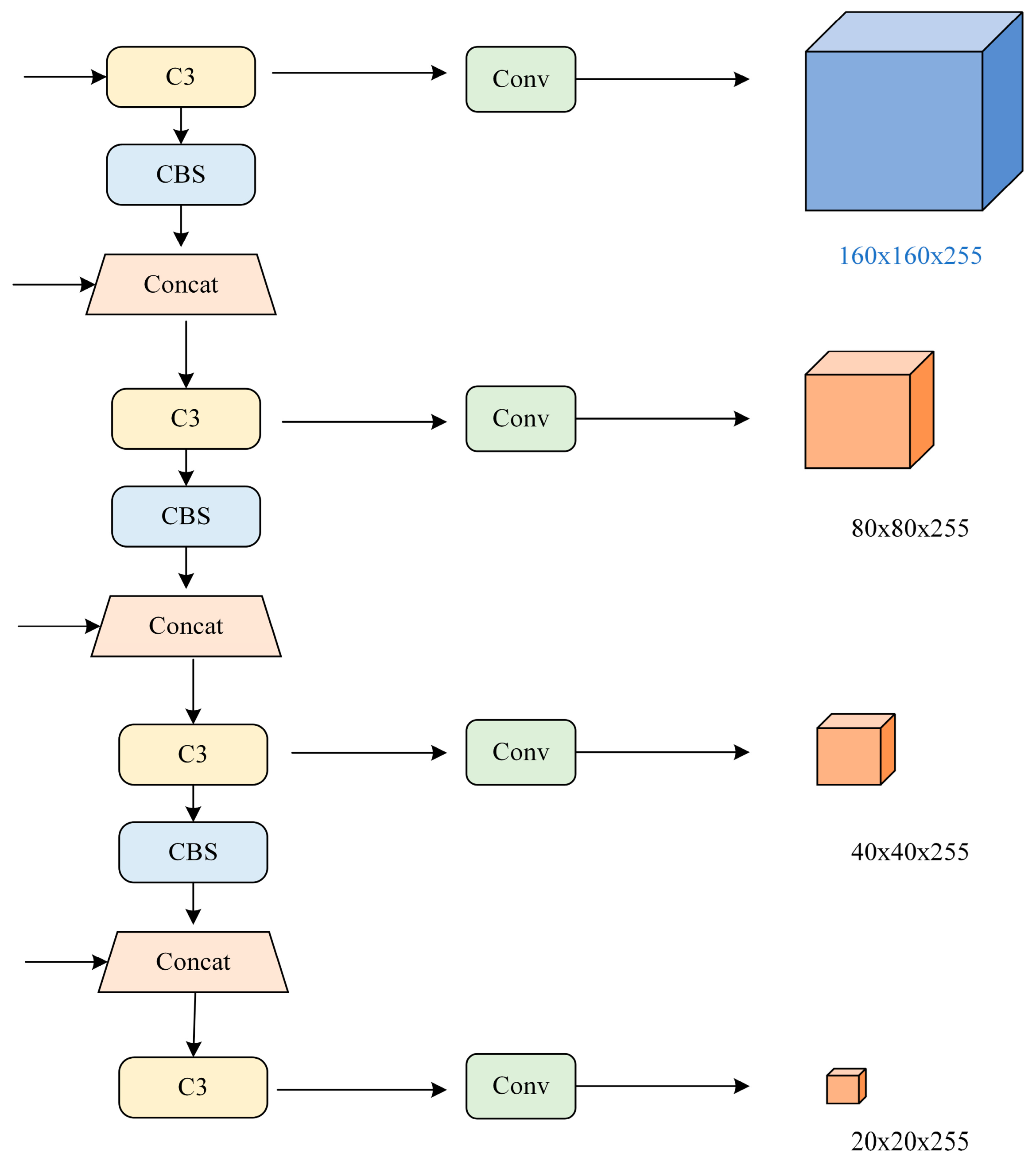
Adding a small target detection layer and embedding an attention mechanism. A 160 × 160 scale output is added to the prediction section, while the ACmix attention mechanism is embedded in front of the 80 × 80 and 160 × 160 scales, which is used to reduce the missed and false detection of small target defects.

(3)

To optimize the prior bounding boxes and loss functions, EIoU Loss is replaced as the loss function of the proposed algorithm. It is more sensitive to the localization accuracy and can better reflect the object shape. Compared with the original loss function, it can make the model converge faster. At the same time, the anchors are clustered using K-means++, which makes the priori bounding boxes match better.

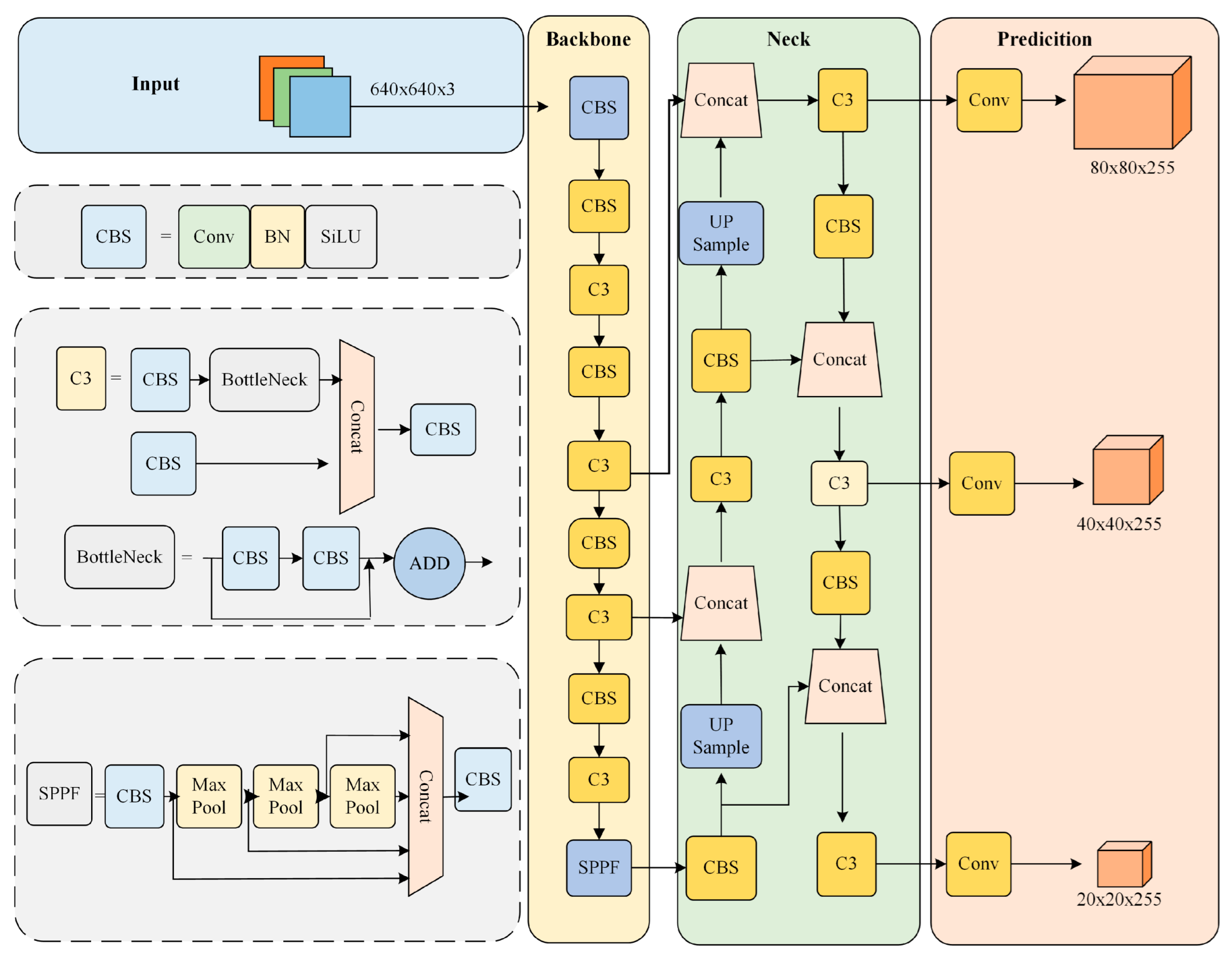
2. Original YOLOv5s and Improved YOLOv5s

Undeniably, the YOLO series has undergone significant advancements in performance through the optimization and iteration of its various versions. From the perspective of the network architecture of the YOLO series, the original YOLOv1 abandoned the traditional sliding window approach, and instead utilized a single convolutional neural network to predict over the entire image. YOLOv2 [21] incorporated the VGG network structure to erect the Darknet-19 backbone network. Similarly, YOLOv3 utilized the residual structure of ResNet to construct a deeper Darknet-53 architecture. YOLOv4 summarized various improvement techniques from YOLOv3 and implemented CSPDarknet-53 as its backbone network, while preserving the fundamental structure observed in YOLOv3. Finally, YOLOv5 constructed five different models, N/S/M/L/X, based on network depths and widths, while retaining a basic structure similar to that of YOLOv4. The YOLOv5 network structure is shown in Figure 1 below.

The YOLOv5 network structure can be divided into the following four main parts: input, backbone, neck and detection. The input side includes adaptive scaling, adaptive anchor box calculation, and Mosaic data enhancement. Adaptive scaling scales the image to a size of 640 × 640 by default, while adaptive anchor frame calculation automatically calculates the optimal anchor frame value for the training set at the training time. Mosaic data augmentation means randomly stitching an input photo with any three other images in the training set by cropping and scaling them into a single image for training. The backbone consists of the CBS, C3 and SPPF module. CBS is composed of a 2D convolutional layer, a BN layer and a SiLU activation function; in the new version, the authors transformed the BottleNeckCSP module into a C3 module, which is the main module for learning on residual features. Its structure has two branches, CBS with Bottleneck as one branch and a separate CBS as the other branch, and then fusion operations are performed on the two branches. SPPF serves the same function as spatial pyram theid pooling (SPP) module to achieve the fusion of local features and global features, differing in structure. Compared to SPP, the SPPF model has a reduced computational. The neck is composed of a feature pyramid network (FPN) [22] and path aggregation network (PAN) [23] structure to form a feature fusion network. Detection head is used for the output of the object detection results.

In order to address the challenges and complexities associated with insulator defect detection, we have made several enhancements to the network structure and bounding box optimization strategy. Firstly, we have improved the model by substituting C3 and standard convolution with C3Ghost and Ghostconv, resulting in a reduction in the parameter count. Secondly, we have enhanced the model’s capability to detect small target features by introducing a 160 × 160 scale small target detection layer. Additionally, we have integrated the ACmix attention mechanism before the prediction parts for the 80 × 80 and 160 × 160 scales. Lastly, we have performed the reclustering of the prior boxes and refined the loss function, taking into account the anchor box scale characteristics of the insulators in the dataset. The specific improved model structure is illustrated in Figure 2, which demonstrates a better trade-off between accuracy and parameter count, making it more suitable for detecting insulator defects.

3. Related Work

3.1. C3Ghost Module

Traditional feature extraction can capture a large amount of feature information and generate redundant data. Some scholars have optimized the network structure and proposed some lightweight network structures such as MobileNet [24] and ShuffleNet [25]. Han et al. [26] proposed a lightweight module Ghost in 2020, which is able to generate more feature maps while reducing the computation and the number of parameters. It works as shown below in Figure 3.

Given input data $X\in R^{c\times h\times w}$, $h$ and $w$ are the height and width of the input data, and $c$ is the number of input data channels. Any convolution operation used to generate an n-feature map can be expressed as follows:

$$Y=X\cdot \omega +b$$

(1)

where $Y\in R^{n\times h^{\prime }\times w^{\prime }}$ represents an n-feature map of height $h^{\prime }$ and width $w^{\prime }$, and $\omega \in R^{c\times k\times k\times n}$ represents the convolution operation performed by $c\times n$ convolution kernels of size $k\times k$.

The working principle of the Ghost module is shown in Figure 3. Firstly, the regular convolution is used to obtain the intrinsic feature map $Y^{\prime }\in R^{n\times h^{\prime }\times w^{\prime }}$, which can be expressed as follows:

$$Y^{\prime }=X\cdot {\omega }^{\prime }$$

(2)

where ${\omega }^{\prime }\in R^{c\times k\times k\times m}$ represents the filters and the bias term is ignored. A series of linear operations are then used to generate repeating features based on the following:

$$Y_{ij}={\mathrm{\Phi }}_{i,j}(Y_i^{\prime }),\forall i=1,\dots m,j=1,\dots s$$

(3)

where $Y_i^{\prime }$ represents the $i$-th feature map in $Y^{\prime }$, and ${\mathrm{\Phi }}_{i,j}$ is the $j$-th linear operation for each $Y_i^{\prime }$ needed to generate the $j$-th Ghost feature map $Y_{ij}$.

Finally, the intrinsic feature maps obtained in the first step and the Ghost feature maps obtained in the second step are spliced to obtain the final output.

After using the Ghost module, the linear convolution kernel size is set to $d\times d$, and the computation of the Ghost module is compared with that of the standard convolution:

$$C_s=\frac{c\cdot k\cdot k\cdot n\cdot h^{\prime }\cdot w^{\prime }}{\frac{n}{s}\cdot h^{\prime }\cdot w^{\prime }\cdot c\cdot k\cdot k+(s-1)\cdot h^{\prime }\cdot w^{\prime }\cdot d\cdot d}=\frac{c\cdot k\cdot k}{c\cdot k\cdot k\cdot \frac{1}{s}+d\cdot d\cdot \frac{s-1}{s}}\approx \frac{s\cdot c}{s+c-1}\approx s$$

(4)

where $d\times d$ and $k\times k$ are of similar size and $s$<<$c$, so it can be calculated that the computation of the Ghost module is 1/s of the standard convolution. The calculation of the parameters is similar, and it can also be simplified to s in the end. Therefore, based on the Ghost module, GhostBottleneck is designed, and the specific structure is shown in Figure 4.

Taking advantage of the Ghost module and GhostBottleneck, we introduce a lightweight feature extraction structure, C3Ghost, which references the structure of CSPNet [27], as shown in Figure 4 below. It consists of three 1 × 1 convolutional layers and n linearly stacked GhostBottleneck. The structure effectively preserves the feature information of the original image and avoids feature loss. The C3ghost module is used to replace all C3 modules in YOLOv5 to reduce the computation and compress the size of the model.

3.2. Detection Layer for Small Object

The YOLOv5 algorithm incorporates a feature fusion structure consisting of FPN and PAN. FPN facilitates the fusion of semantic information from deeper layers to shallower layers, thereby constructing multi-scale feature maps. This approach enriches the feature representation and aids in small-object detection, as well as object detection in complex scenes. In contrast to FPN, PAN fuses location information from shallower layers to deeper layers, which enhances location information at various scales. This process is especially crucial for small objects that do not provide sufficient space for high-resolution location information. In such cases, accurately locating the object position becomes pivotal, and the effective combination of semantic and location information is key to improving the detection performance.

Considering that the defect types in the collected insulator dataset are mostly small objects, a 160 × 160 small-object detection layer is added to the improved model for enhancing the perception of small objects. As shown in Figure 5, four different scales of detection layers, namely 160 × 160, 80 × 80, 40 × 40 and 20 × 20, are obtained.

3.3. On the Integration of Self-Attention and Convolution

The attention mechanism is designed to concentrate on local information and make the model more focused on the detection of object features. In object detection tasks, the object being detected may not always be positioned at a fixed location in the image, and its location and percentage in the image may vary depending on the environmental conditions during capture. As such, the attention area dynamically changes based on the detection task. In the dataset used for this study, insulator defects are small objects that require careful feature extraction. Therefore, attention is employed to focus more on this portion of the features.

ACmix [28] integrates the advantages of convolutional and transformer networks to improve the network performance with low computational overhead. ACmix consists of two stages, as shown in Figure 6; the first stage is projected with a 1 × 1 convolution to obtain the intermediate feature set, and then, the second stage follows two different pairs of modes, self-attentive and convolutional, to perform feature aggregation and reuse. In this way, ACmix has the advantage of two modules and avoids performing the highly complex projection operation twice.

On the self-attentive path, ACmix collects the intermediate features into N groups; each group contains three features corresponding to three feature mappings, namely query, key and value, following the self-attentive modular approach used to collect information. Let $f_{ij}$ and $g_{ij}$ denote the tensor corresponding to the input and output of pixel $(i,j)$, and $N_k(i,j)$ denote the local pixel region with $(i,j)$ as the center and spatial width $k$. Then $\mathrm{A}\left(W_q^{(l)}{f}_{ij},W_k^{(l)}{f}_{ab}\right)$ is the tensor about $N_k(i,j)$ corresponding weights, and the formula is shown in Equation (5):

$$\mathrm{A}\left(W_q^{(l)}{f}_{ij},W_k^{(l)}{f}_{ab}\right)=\underset{{\mathcal{N}}_k(i,j)}{\mathrm{softmax}}\left(\frac{{\left(W_q^{(l)}{f}_{ij}\right)}^{\mathrm{T}}\left(W_k^{(l)}{f}_{ab}\right)}{\sqrt{d}}\right)$$

(5)

where $W_q^{(l)}$ and $W_k^{(l)}$ are the projection matrices of query and key, and $d$ is the characteristic dimension of $W_q^{(l)}{f}_{ij}$.

In ACmix, the multi-headed self-attention can be decomposed into two stages, as shown in Equations (6) and (7).

$$q_{ij}^{(l)}=W_q^{(l)}{f}_{ij},k_{ij}^{(l)}=W_k^{(l)}{f}_{ij},v_{ij}^{(l)}=W_v^{(l)}{f}_{ij}$$

(6)

$$g_{ij}=\underset{l=1}{\overset{N}{\Vert }}\left({\displaystyle \sum }_{a,b\in N_{k(i,j)}}A\left(q_{ij}^{(l)},k_{ab}^{(l)}\right)v_{ab}^{(l)}\right)$$

(7)

where $W_q^{(l)}$ is the projection matrix of value, and $q_{ij}^{(l)}$, $k_{ij}^{(l)}$ and $v_{ij}^{(l)}$ are the query, key, and value matrices, respectively. $\Vert$ is the cascade of N attention head outputs.

On the Self-Attention path, the intermediate features are aggregated into $N$ groups, where each group contains three feature maps from a 1 × 1 convolution, which are used as query, key, and value. On another convolution path with kernel $k$, a fully connected layer is used and $k^2$ feature maps are generated. Finally, the outputs of the two paths are summed, and the intensity is controlled using two learnable scalars control:

$$F_{out}=\alpha F_{att}+\beta F_{conv}$$

(8)

where $F_{out}$ is the final output of the path, $F_{att}$ is the output of the self-attentive path, and $F_{conv}$ is the output of the convolutional path. The values of the parameters $\alpha$ and $\beta$ are 1.

The ACmix mechanism enhances the flexibility of the network by extracting richer features from the feature map. This enables the model to pay more attention to the defects of electrical equipment, thereby improving its ability to accurately distinguish small objects from the background and reducing the rate of missed detections. By striking a balance between the features of large-scale and small-scale objects, the input feature network becomes more balanced, leading to improved overall performance in detecting various object sizes.

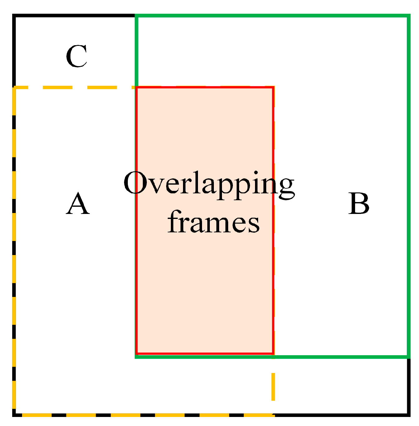
3.4. Optimization of Loss Function

The Generalized IoU (GIoU) Loss function is used in YOLOv5s. A schematic diagram of the IoU is shown in Figure 7. GIoU is based on IoU, and introduces the area of the smallest rectangular box enclosed by both $A$ and $B$ into the calculation of the loss function; the calculation formula is shown in Equation (9):

$$GIo{U}_{\mathrm{loss}}\left(A,B\right)=1-\left(IoU\left(A,B\right)\right)-\frac{\left|C-\left(A\cap B\right)\right|}{\left|C\right|}$$

(9)

where $A$ and $B$ denote the actual object frame and the predicted object frame, respectively, C denotes the minimum peripheral rectangle containing $A$ and $B$, and $A\cap B$ is the overlapping region of the actual and predicted frames. The object loss is represented by the binary cross-entropy loss, whose formula is shown in Equation (10). Here, 0 denotes no object and 1 denotes an object.

$$L_{\mathrm{obj}}=-\left[y\log x+(1-y)\log (1-x)\right]$$

(10)

where $L_{\mathrm{obj}}$ is the object loss, $y$ is the true label, which takes the value of 1, and $x$ is the predicted label, which takes the value of 0 or 1. The category loss $L_{\mathrm{cls}}$ has the same formula form as the object loss, but $x$ takes the value between [0, 1] for calculating the loss of the category to which the object belongs, and consists of a binary cross-entropy loss function. The total loss is shown in Equation (11).

$$L_{\mathrm{loss}}=GIo{U}_{\mathrm{loss}}+L_{\mathrm{obj}}+L_{\mathrm{cls}}$$

(11)

Since the loss function GIoU degenerates into IoU when the detection frame and the real frame contain the phenomenon, and the convergence speed is slow when the two frames intersect, the EIoU [29] loss function is used to replace the GIoU loss function. Its calculation formula is shown as follows:

$$L_{\mathrm{EIoU}}=1-IoU+\frac{{\rho }^2\left(b,b^{\mathrm{gt}}\right)}{c^2}+\frac{{\rho }^2\left(w,w^{\mathrm{gt}}\right)}{c_{\mathrm{w}}^2}+\frac{{\rho }^2\left(h,h^{\mathrm{gt}}\right)}{c_h^2}$$

(12)

where $b$, $w$, and $h$ denote the center point, width, and height of the prediction box, and $b^{\mathrm{gt}}$, $w^{\mathrm{gt}}$ and $h^{\mathrm{gt}}$ denote the center point, width, and height of the real box, respectively; $c_{\mathrm{w}}^{}$ and $c_h$ are the width and height of the minimum external box covering the prediction box and the real box.

The EIoU Loss is a loss function that addresses the limitations of traditional IoU calculation in bounding box regression. It considers factors such as relative position, scale, and aspect ratio between the predicted bounding box and the ground truth bounding box, leading to improved accuracy in bounding box positioning. By introducing penalty terms for factors such as position, scale, and aspect ratio into the IoU calculation, the EIoU Loss overcomes the issue of gradient vanishing during gradient regression, which can hinder model convergence. This enhanced loss function improves the IoU calculation by incorporating additional terms and effectively avoids the gradient vanishing problem, thereby accelerating model convergence. As a result, the EIoU Loss replaces the original loss function, offering better regression accuracy and faster training convergence in object detection tasks.

3.5. Optimisation of Anchor Frame Clustering

The YOLOv5 algorithm utilizes the K-means algorithm to cluster the anchor frames of the dataset and obtain the initial anchor frame parameters. However, the random assignment of initial clustering centers in the K-means algorithm can result in a significant gap between the initial centers and the optimal centers. This can lead to increased volatility in the coordinate prediction of the output anchor frames and can subsequently affect the positioning accuracy. To overcome the limitations of the K-means clustering algorithm, we propose using the K-means++ algorithm as a replacement in the original algorithm. The K-means++ algorithm improves the selection of random initial points in a more intuitive and effective manner. By redesigning the size of the pre-verification box through clustering analysis on the dataset, we can achieve a higher degree of matching between the pre-verification box and the target bounding box. This enhancement helps to improve the accuracy of the positioning process. The k-means++ algorithm works as shown below:

1.

Determine the number of clustering centers k and the set of heights and widths $M$ for the dataset in this paper.

2.

Randomly choose a point from the set $M$ to satisfy the initial clustering center $q_1$.

3.

Determine the distance between each remaining point x in the set M of $D\left(x\right)$ and its nearest clustering center $q_x$. The greater the distance between the previous box and the next clustering center, the greater the probability $P\left(x\right)$. This step should be repeated until k clustering centers are found.

$$D\left(x\right)=1-IoU\left(x,q_x\right)$$

(13)

$$P\left(x\right)=\frac{D{\left(x\right)}^2}{{{\displaystyle \sum }}_{x\in N}D{\left(x\right)}^2}$$

(14)

$IoU\left(x,q_x\right)$ denotes the intersection ratio between the clustering center and each labeled box.

4.

Determine the distance $D\left(x\right)$ between all points in the set $M$ and the $k$ cluster centers, and place the point in the category of cluster centers with the smallest distance. For the clustering results, recalculate each cluster category center $C_i$.

$$C_i=\frac{{{\displaystyle \sum }}_{x\in C_i}x}{\left|C_i\right|}$$

(15)

5.

When the cluster center $C_i$ of each clustering category no longer changes, repeat Step 2 and output $k$ cluster center results.

A comparison of the two clustering algorithms is shown in

Table 1. Comparison of clustering algorithms.

Clustering Algorithm	Recall	Fitness	Anchors
K-means	0.9952	0.74872	(13, 12) (26, 16) (17, 25)
			(36, 29) (120, 24) (71, 45)
			(37, 149) (187, 42) (409, 97)
K-means++	0.9981 (+0.29%)	0.77200 (+2.32%)	(13, 13) (25, 18) (17, 70)
			(43, 31) (117, 23) (115, 41)
			(45, 165) (364, 52) (421, 71)
			(402, 93) (427, 130) (365, 191)

, where Fitness indicates how well the a priori anchors match the target boxes to be detected in the dataset. Compared to k-means, the Recall metric of K-means++ improves by 0.29% and the fitness metric improves by 2.32%. Additionally, the number of preset anchor frames increases from 9 to 12 as a result of incorporating a new detection layer into the enhanced network. This improved clustering method successfully generates more precise anchor frames.

4. Experiment and Analysis

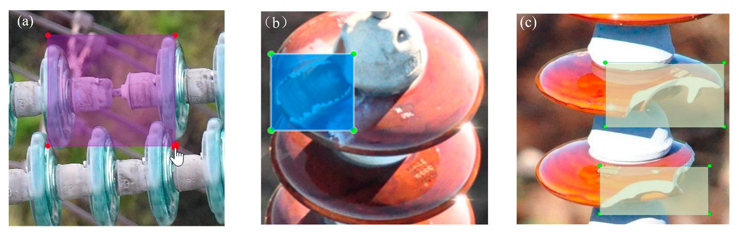
4.1. Data Acquisition and Pre-Processing

The dataset used in the experiment consists of two parts. One part comes from the public dataset CPLID provided by the National Grid, with an image size of 1152 × 864 px and a total of 848 images. The other part comes from the collection of inspection drones with image sizes of 6016 × 4016 px and 3216 × 2136 px, containing glass insulators and porcelain insulators, totaling 1642 images. The specific types of defects are shown in Figure 8. LabelImg was used to annotate the data. The data were labeled as ‘insulator’, ‘defect’, ‘flashover damage’, and ‘broken’, according to 4 types.

After filtering using data enhancement, a total of 4034 images containing normal insulators and images containing three types of defective insulators were obtained. The labeling of each image was performed one by one to obtain the labeled insulator dataset. Then, the training set, test set and validation set were randomly divided in the ratio of 8:1:1. Where Figure 9 shows the mosaic data enhancement method that increases the number of small target samples in the dataset.

4.2. Experiment Environment

This experiment was conducted within the Pytorch framework, running in the Window 10 environment. The specific hardware environment for the experiment was as follows: CPU model was 12th Gen Intel(R) Core (TM) i5-12500H, graphics card type was GeForce RTX 3050 Laptop GPU, video memory size was 4G, and memory size was 16 G. Initial learning rate was 0.001.

4.3. Evaluation Metrics of the Model

In this experiment, the detection evaluation metrics included Precision, Recall, AP, mAP, number of parameters and FPS. The specific calculation formula for each metric was calculated as follows:

$$Precision=\frac{T_P}{T_P+F_P}\times 100\%$$

(16)

$$Recall=\frac{T_P}{T_P+F_N}$$

(17)

$$AP={{\displaystyle \int }}_0^{1}P\left(R\right)\mathrm{d}R$$

(18)

$$mAP=\frac{{{\displaystyle \sum }}_{i=1}^{N}A{P}_i}{N}$$

(19)

where $T_p$ is the number of correctly predicted positive samples, $F_p$ is the number of incorrectly predicted positive samples, and $F_N$ is the number of incorrectly predicted negative samples. $AP$ is the P-R curve integral, and $mAP$ is the average accuracy over all categories, used to find the mean value.

4.4. Analysis of Experimental Results

In order to reflect how well the original YOLOv5s model classifies under the self-constructed dataset, and determine whether there are certain categories that are easily misclassified or missed by the model, we plotted the confusion matrix of the original YOLOv5s as shown in Figure 10 to provide guidance for us to improve the model, where the horizontal coordinates represent the predicted values and the vertical coordinates represent the true values; the background is also included as a category in the model evaluation in the confusion matrix.

From the data in Figure 10 of the confusion matrix of the original YOLOv5s, it can be observed that the model can achieve a high level of classification accuracy, but that there are still some missed detections; this is related to the self-built dataset containing more small objects and overlapping objects. The recognition rate of all kinds of objects in the insulator dataset reaches more than 89%, among which the recognition rate of insulators is as high as 98%. However, the misidentification rate of insulators is as high as 49%, and the misidentification rate of insulator flashover defects is as high as 41%. This indicates that the complex background and dense small objects interfere in the recognition rate.

Ablation experiments were used to verify the algorithm performance, and the effect of adding or modifying each part of the structure on each evaluation index was verified separately. In the initial A, B, and C experiments, Group A has an input scale of 320 × 320, Group B has a default input scale of 640 × 640, and Group C has an input scale of 1280 × 1280. The mAP variation curves at different scales are shown in Figure 11 below Our primary aim was to investigate the influence of varying input scales on the algorithm’s performance. The experimental results show that choosing different input scales has an effect on the accuracy of the model. Larger input scales contain more feature map details and have greater accuracy. However, there is some saturation as the scale expands, and the change in accuracy is not obvious when the scale already contains most of the feature map details. Moreover, considering that a larger input scale increases the computational consumption, in order to achieve a balance, this paper adopts the 640 × 640 scale.

The results of the Group D experiment in

Table 2. Results of ablation experiments.

Group	Model	Precision (%)	Recall (%)	mAP@0.5 (%)	Parameters (M)	FPS (f/s)
A	YOLOv5s (320 × 320)	89.1	80.3	83.9	7.03	32.89
B	YOLOv5s (640 × 640)	95.4	91.9	94.6	7.03	32.36
C	YOLOv5s (1280 × 1280)	96.3	94.2	96.2	7.03	31.84
D	YOLOv5s (640) + C3Ghost	93.4	89.1	92.2	3.69	35.21
E	YOLOv5s (640) + C3Ghost + 4Head	93.0	89.4	92.4	4.06	33.22
F	YOLOv5s (640) + C3Ghost + 4Head + ACmix	95.0	90.4	93.5	4.14	32.89
G	YOLOv5s (640) + C3Ghost + 4Head + ACmix + EIoU+K-means++	95.8	92.2	94.8	4.14	32.52

show that replacing lightweight modules C3Ghost and GhostConv resulted in a 47.5% reduction in model parameters and improved FPS metrics. However, this improvement came at the cost of decreased detection precision. To address this issue, we introduced a small target detection layer in Group E. The evaluation results in Figure 12 demonstrate that the AP values for the “flashover” and “broken” defects categories were improved by 1.8% and 1.5%, respectively.

In Group F, we further improved the detection performance of small targets by adding the ACmix attention mechanism. Moving on to Group G, we employed EIoU Loss and K-means++ techniques to optimize the calculation and matching of anchor frames. This approach resulted in a 0.8% increase in the inspection precision, a 2.2% increase in recall, and a 1.5% increase in mAP@0.5, with the same number of parameters as Group F. These findings indicate that incorporating these advanced techniques can significantly enhance the performance of object detection while maintaining the parameter constant.

The change in the loss values before and after replacing the loss function is shown in Figure 13; the horizontal coordinates in the figure are epoch and the vertical coordinates are loss values. After changing the original loss function to EIoU, its convergence speed is faster than the original algorithm and its loss value is lower than the original aorithm.

Using the experiment of group B as the control benchmark, the improved algorithm improves the AP values of “defect” and “flashover” by 4.1% and 1.8%, respectively, and slightly improves the precision, recall, and mAP@0.5 compared with group B. The number of parameters decreases by 41.1%.

To validate the performance superiority of our enhanced algorithm, we conducted a comparative evaluation of its defect detection capabilities against similar algorithms using an identical dataset.

Table 3. Comparison of detection results of other algorithms of the same type.

Model	Input Size	Precision (%)	Recall (%)	mAP@0.5 (%)	Parameters (M)
Faster R-CNN	640 × 640	96.8	93.2	95.5	108.9
SSD	640 × 640	88.7	85.2	88.6	26.93
Centernet	640 × 640	95.3	87.9	94.5	32.45
YOLOv3	640 × 640	95.6	91.7	93.8	61.7
YOLOv3-tiny	640 × 640	91.2	86.8	90.2	8.7
YOLOv5s	640 × 640	95.4	91.9	94.6	7.03
YOLOv7	640 × 640	94.7	90.9	93.7	37.2
YOLOv8s	640 × 640	96.9	93.8	96.4	11.14
Ours	640 × 640	96.2	92.9	94.8	4.14

summarizes the corresponding experimental outcomes. Our proposed algorithm outperformed SSD, YOLOv3, YOLOv3-tiny, and YOLOv7 [30] by reporting mAP@0.5 values that were 6.2%, 1%, 4.6%, and 1.1% higher than these algorithms, respectively. Additionally, the precision and recall rates of our algorithm were also superior to those of these algorithms, complemented by the smallest number of model parameters compared to the other tested models. Although the detection precision is slightly lower compared to YOLOv8s, the number of parameters of the improved algorithm is significantly lower than that of YOLOv8s. These empirical results confirm that our algorithm strikes a better balance between the number of parameters in the model and the detection precision, producing a smaller number of parameters while still maintaining a high detection precision.

In order to assess the effectiveness of the enhanced algorithm, we selected validation images showing insulators with diverse types of defects in various scenarios. Figure 14 shows the detection results of our algorithm for these selected images. Achieving better detection with a small number of defect types, Figure 15 presents our improved algorithm’s high detection accuracy, even under complex conditions in which multiple defective insulators coexist with small objects and diverse backgrounds. These results validate the efficacy of our algorithm in identifying small-object defects, with only a few missed detections observed. Moreover, as shown in Figure 16, our algorithm’s robust detection performance remains unaffected even when encountering fogged insulators, highlighting its exceptional anti-interference ability.

5. Conclusions

In this paper, we propose a novel lightweight approach to insulator defect detection based on the improved YOLOv5s algorithm. To meet the deployment needs of edge devices, we first incorporate the C3Ghost module, which offers similar feature extraction capabilities but with reduced network parameters. Additionally, we introduce a small-target detection layer and add the ACmix attention mechanism to enhance the ability to focus on small-target features and reduce the missing detection of small-target defects. Furthermore, we employ the K-means++ clustering algorithm using the dataset provided in this study to optimize the re-clustering of prior frames. Simultaneously, the computation of anchor frames is refined, utilizing the EIoU loss function to achieve superior localization accuracy and faster convergence. The experimental results demonstrate that the proposed algorithm exhibits a low parameter count while meeting the detection performance requirements outlined in the dataset for this study. However, it is worth noting that under foggy conditions, there were instances of missed detections, particularly for densely packed small objects. Future research efforts will target enhancing feature fusion across different scales to address this limitation and further improve the overall model performance.

References

1. Yang, L.; Fan, J.; Liu, Y. A review on state-of-the-art power line inspection techniques. IEEE Trans. Instrum. Meas. 2020, 69, 9350–9365. [Google Scholar] [CrossRef]
2. Liu, J.J.; Liu, C.A.Y.; Wu, Y.Q. An Improved Method Based on Deep Learning for Insulator Fault Detection in Diverse Aerial Images. Energies 2021, 14, 4365. [Google Scholar] [CrossRef]
3. Xiao, Y.Z.; Tian, Z.Q.; Yu, J.C. A review of object detection based on deep learning. Multim. Tools Appl. 2020, 79, 23729–23791. [Google Scholar] [CrossRef]
4. Girshick, R.; Donahue, J.; Darrell, T.; Malik, J. Rich feature hierarchies for accurate object detection and semantic segmentation. In Proceedings of the IEEE Conference on Computer Vision and Pattern Recognition, Columbus, OH, USA, 23–28 June 2014; pp. 580–587. [Google Scholar]
5. Girshick, R. Fast r-cnn. In Proceedings of the 2015 IEEE Conference on Computer Vision and Pattern Recognition (CVPR), Boston, MA, USA, 8–10 June 2015; pp. 1440–1448. [Google Scholar]
6. Ren, S.; He, K.; Girshick, R.; Sun, J. Faster R-CNN: Towards Real-Time Object Detection with Region Proposal Networks. IEEE Trans. Pattern Anal. Mach. Intell. 2017, 39, 1137–1149. [Google Scholar] [CrossRef]
7. Guo, Z.M.; Tian, Y.Y.; Mao, W.D. A Robust Faster R-CNN Model with Feature Enhancement for Rust Detection of Transmission Line Fitting. Sensors 2022, 22, 7961. [Google Scholar] [CrossRef]
8. Ou, J.H.; Wang, J.G.; Xue, J. Infrared Image Target Detection of Substation Electrical Equipment Using an Improved Faster R-CNN. IEEE Trans. Power Deliv. 2023, 38, 387–396. [Google Scholar] [CrossRef]
9. Liu, W.; Anguelov, D.; Erhan, D. SSD: Single shot multibox detector. In Proceedings of the 2016 European Conference on Computer Vision (ECCV), Amsterdam, The Netherlands, 8–16 October 2016; pp. 21–37. [Google Scholar]
10. Lin, T.-Y.; Goyal, P.; Girshick, R.; He, K.; Dollár, P. Focal loss for dense object detection. arXiv 2017, arXiv:1708.02002. [Google Scholar]
11. Redmon, J.; Divvala, S.; Girshick, R. You only look once: Unified, real-time object detection. In Proceedings of the 2016 IEEE Conference on Computer Vision and Pattern (CVPR), Las Vegas, NV, USA, 26 June–1 July 2016; pp. 779–788. [Google Scholar]
12. Wei, B.Q.; Xie, Z.X.; Liu, Y.D. Online Monitoring Method for Insulator Self-explosion Based on Edge Computing and Deep Learning. CSEE J. Power Energy Syst. 2022, 8, 1684–1696. [Google Scholar]
13. Liu, C.Y.; Wu, Y.Q.; Liu, J.J. Improved YOLOv3 Network for Insulator Detection in Aerial Images with Diverse Background Interference. Electronics 2021, 10, 771. [Google Scholar] [CrossRef]
14. Yang, Z.S.; Xu, Z.; Wang, Y.H. Bidirection-Fusion-YOLOv3: An Improved Method for Insulator Defect Detection Using UAV Image. IEEE Trans. Instrum. Meas. 2022, 71, 3521408. [Google Scholar] [CrossRef]
15. Han, G.J.; Zhao, L.; Li, Q. A Lightweight Algorithm for Insulator Target Detection and Defect Identification. Sensors 2023, 23, 1216. [Google Scholar] [CrossRef] [PubMed]
16. Bochkovskiy, A.; Wang, C.-Y.; Liao, H.-Y.M. Yolov4: Optimal speed and accuracy of object detection. arXiv 2020, arXiv:2004.10934. [Google Scholar]
17. Redmon, J.; Farhadi, A. Yolov3: An incremental improvement. arXiv 2018, arXiv:1804.02767. [Google Scholar]
18. Ding, J.; Cao, H.A.; Ding, X.L. High Accuracy Real-Time Insulator String Defect Detection Method Based on Improved YOLOv5. Front. Energy Res. 2022, 10, 928164. [Google Scholar] [CrossRef]
19. Li, Y.H.; Zou, G.P.; Zou, H.L. Insulators and Defect Detection Based on the Improved Focal Loss Function. Appl. Sci. 2022, 12, 10529. [Google Scholar] [CrossRef]
20. Zhang, Z.D.; Zhang, B.; Lan, Z.C. FINet: An Insulator Dataset and Detection Benchmark Based on Synthetic Fog and Improved YOLOv5. IEEE Trans. Instrum. Meas. 2022, 71, 6006508. [Google Scholar] [CrossRef]
21. Redmon, J.; Farhadi, A. YOLO9000: Better, faster, stronger. In Proceedings of the 30th IEEE Conference on Computer Vision and Pattern Recognition, Honolulu, HI, USA, 21–26 July 2017; pp. 7263–7271. [Google Scholar]
22. Lin, T.-Y.; Dollár, P.; Girshick, R.; He, K.; Hariharan, B.; Belongie, S. Feature pyramid networks for object detection. In Proceedings of the 30th IEEE Conference on Computer Vision and Pattern Recognition, Honolulu, HI, USA, 21–26 July 2017; pp. 2117–2125. [Google Scholar]
23. Liu, S.; Qi, L.; Qin, H.; Shi, J.; Jia, J. Path aggregation network for instance segmentation. In Proceedings of the IEEE Conference on Computer Vision and Pattern Recognition, Salt Lake City, UT, USA, 18–23 June 2018; pp. 8759–8768. [Google Scholar]
24. Howard, A.G.; Zhu, M.; Chen, B.; Kalenichenko, D.; Wang, W.; Weyand, T.; Andreetto, M.; Adam, H. Mobilenets: Efficient convolutional neural networks for mobile vision applications. arXiv 2017, arXiv:1704.04861. [Google Scholar]
25. Zhang, X.; Zhou, X.; Lin, M.; Sun, J. Shufflenet: An extremely efficient convolutional neural network for mobile devices. In Proceedings of the 2018 IEEE/CVF Conference on Computer Vision and Pattern Recognition, Salt Lake City, UT, USA, 18–23 June 2018; pp. 6848–6856. [Google Scholar]
26. Han, K.; Wang, Y.; Tian, Q.; Guo, J.; Xu, C.; Xu, C. Ghostnet: More features from cheap operations. In Proceedings of the IEEE/CVF Conference on Computer Vision and Pattern Recognition, Seattle, WA, USA, 14–19 June 2020; pp. 1580–1589. [Google Scholar]
27. Wang, C.-Y.; Liao, H.-Y.M.; Wu, Y.-H.; Chen, P.-Y.; Hsieh, J.-W.; Yeh, I.-H. CSPNet: A new backbone that can enhance learning capability of CNN. In Proceedings of the IEEE/CVF Conference on Computer Vision and Pattern Recognition Workshops, Seattle, WA, USA, 14–19 June 2020; pp. 390–391. [Google Scholar]
28. Pan, X.; Ge, C.; Lu, R.; Song, S.; Chen, G.; Huang, Z.; Huang, G. On the integration of self-attention and convolution. In Proceedings of the IEEE/CVF Conference on Computer Vision and Pattern Recognition, New Orleans, LA, USA, 19–20 June 2022; pp. 815–825. [Google Scholar]
29. Zhang, Y.-F.; Ren, W.; Zhang, Z.; Jia, Z.; Wang, L.; Tan, T.J.N. Focal and efficient IOU loss for accurate bounding box regression. arXiv 2022, arXiv:2101.08158. [Google Scholar] [CrossRef]
30. Wang, C.Y.; Bochkovskiy, A.; Liao, H. YOLOv7: Trainable bag-of-freebies sets new state-of-the-art for real-time object detectors. arXiv 2022, arXiv:2207.02696. [Google Scholar]
Figure 1. YOLOv5 network structure.
Electronics 12 04292 g001
Figure 2. Improved YOLOv5s structure diagram.
Electronics 12 04292 g002
Figure 3. Standard convolution and Ghost module.
Electronics 12 04292 g003
Figure 4. C3Ghost structure diagram.
Electronics 12 04292 g004
Figure 5. Structural diagram of the four detection scales.
Electronics 12 04292 g005
Figure 6. ACmix structure diagram.
Electronics 12 04292 g006
Figure 7. IoU diagram.
Electronics 12 04292 g007
Figure 8. Examples of defect types for insulator. (a) Self-explosion. (b) Flashover. (c) Broken.
Electronics 12 04292 g008
Figure 9. Mosaic data enhancement method.
Electronics 12 04292 g009
Figure 10. Confusion matrix of the original YOLOv5s.
Electronics 12 04292 g010
Figure 11. Variation curves of mAP for different input scales. (a) mAP@0.5; (b) mAP@0.5:0.95.
Electronics 12 04292 g011
Figure 12. AP value for each type of defect.
Electronics 12 04292 g012
Figure 13. Loss value curve of GIoU and EIoU.
Electronics 12 04292 g013
Figure 14. Detection effect of various defects.
Electronics 12 04292 g014
Figure 15. Detection effect of dense small objects.
Electronics 12 04292 g015
Figure 16. Detection effect under foggy conditions.
Electronics 12 04292 g016