Research on Automatic Vertical Parking Path-Planning Algorithms for Narrow Parking Spaces

Abstract

Narrow parking spaces pose difficulties in path planning and spot turning caused by sudden changes and discontinuities in path curvature. To address these problems, this paper investigates the performance of three path-planning algorithms and proposes a path-optimization algorithm. First, a narrow parking space is defined based on single-step parking using the arc-line combination parking algorithm. Second, to compare the arc-line combination algorithm, Hybrid A* algorithm, and particle swarm optimization parking algorithm with respect to different narrow parking spaces, a multi-objective evaluation function is proposed, including three evaluation indicators, namely, the path length, the number of positive and negative conversions of vehicle speed, and the smoothness of the path. Their performance is compared using a simulation conducted in MATLAB. With the same starting point and different parking space widths, the three algorithms are simulated to generate different planned paths. Then, the evaluation indices are obtained to compare the performance of the algorithms based on the multi-objective function, the values of which indicate the fitness of the algorithm in a narrow parking environment. The results show that the Hybrid A* algorithm is better than the others for narrow parking spaces. Third, to smooth the planning path, a path optimization algorithm based on the cubic B-spline curve and gradient descent is proposed. Finally, the results of a simulation conducted on the proposed algorithm and the Hybrid A* algorithm are provided: the average minimum curvature of the path was reduced by 0.005 m⁻¹, and the path meets the requirements of the minimum turning radius constraint of the analyzed vehicle. The results show that the proposed algorithm can effectively eliminate the curvature mutation point and constrain the path curvature to meet the requirements of a smooth path.

1. Introduction

With the continuous rise in car ownership, the availability of parking spaces is decreasing, leading to increasingly narrow parking areas and thus rendering parking difficult and inefficient for drivers, even resulting in collisions between a vehicle and surrounding objects. Additionally, this can also cause traffic jams and even traffic accidents. Therefore, automatic parking technology for narrow parking spaces has gradually become a research focus [1].

Automatic parking systems use vehicle sensors to measure the relative distance, speed, and angle between a vehicle and surrounding objects. These measurements are processed either on-board or on a cloud-computing platform. Based on this information, the system controls the vehicle’s steering, acceleration, and deceleration to achieve automatic parking. The parking process can be divided into four steps, namely, environmental perception, parking space detection and recognition, parking path planning, and parking path following control. Among them, path planning consists of planning a path avoiding collision under vehicle dynamics constraints based on environment and location information, and it is executed on the vehicle [2,3].

At present, there are three kinds of vertical parking path-planning algorithms commonly used for traditional standard parking spaces [4]. One is the geometric algorithm. Zhao, B et al. [5] used arc lines as transition paths in local path planning to park a vehicle, including arcs and line segments based on the optimal parking starting point node. Although the parking path was shortened, this method is only suitable for single-step parking. Jiang, M et al. [6] proposed a vertical parking path-planning algorithm based on polynomial curve optimization to improve the safety and success rate of automatic vertical parking in complex environments. Although it can solve the problem of not being able to perform single-step parking, this algorithm requires a wider parking space. Zhang, J et al. [7] proposed a vertical parking trajectory-planning algorithm based on a cycloid curve, decoupling the vertical parking trajectory-planning problem into a path-planning problem and a velocity-planning problem, but it can only be used in slightly narrow parking spaces. The arc–line combination algorithm in the geometric algorithm has accurate characteristics, allowing it to accurately calculate the driving trajectory of a vehicle in the parking process so that the vehicle can accurately park in a specified parking space.

The second is a random search algorithm. Yu, L et al. [8] used a particle swarm optimization algorithm to solve equality constraints based on parking boundaries and inequality constraints based on curvature, collision avoidance, and parking space reduction. It yielded optimized, smooth, and curvature-continuous programmed path curve expressions by taking the weighted sum of the maximum curvature and the absolute value of the horizontal coordinate of the starting position of parking as the objective function. However, due to the large number of parameters involved, its path search efficiency is low. Kim, M et al. [9] proposed a Target Tree RRT* algorithm for complex environments that uses the clothoid path to design a target tree to deal with curvature discontinuity. To further reduce the planning time, a cost function was defined to initialize an appropriate target tree considering obstacles. Combining the optimal variable RRT and searching for the shortest path, the Target Tree RRT* algorithm obtains an approximately optimal path as the sampling time increases. Although the path search time is shortened, the smoothness of the path cannot be guaranteed. Zhang, J et al. [10] proposed a parallel parking path-planning algorithm based on improved particle swarm optimization; comprehensively considered the non-holonomic kinematic constraints of a 4 WS by-wire vehicle, the process constraints and boundary constraints of the power and steering subsystems, obstacle avoidance constraints, the initial parking posture, and target parking posture constraints; and established a parallel parking path-planning constraint optimization problem to minimize the total duration of the parking process. The particle swarm optimization algorithm, which can deal with equality constraints and inequality constraints, was used to solve the problem and determine the optimal parallel parking path. Although it can solve the problem of non-smooth paths, it is not suitable for narrow parking spaces. The search process of the particle swarm optimization algorithm in the random search algorithm is a parallel search. Its computational efficiency is high, and the parking path that meets the conditions can be found in a short time. The principle of the particle swarm optimization algorithm is simple, and the parameter adjustment procedure is relatively simple. For different parking scenarios, only a few parameters need to be adjusted.

The third type is the graph search algorithm. Sedighi, S et al. [11] proposed an efficient computational algorithm that combines the Hybrid A* search algorithm with visibility graph planning to find the shortest non-holonomic path in a mixed (continuous–discrete) environment for automatic parking; although it allows for a relatively short path to be searched for, the search time is increased. Bai, J et al. [12] proposed a directed Hybrid A* global path-planning algorithm based on the generalized Vinor map for the path-planning problem of autonomous valet parking systems. It accurately and effectively generates a collision-free path from the entrance of a parking lot to the starting point of parking. Xiong, L et al. [13] improved the Hybrid A* by adding a penalty term for obstacle distance on the Reeds–Shepp (RS) curve, which ameliorated the problem of the RS curve being too close to obstacles and improved the effectiveness of parking. The Hybrid A* algorithm in the graph search algorithm conducts a heuristic search in a continuous coordinate system, which can ensure that the generated trajectory satisfies a vehicle’s non-integrity constraint (kinematic constraint). It can deal with non-smooth obstacles and find the optimal global solution. By combining the discrete node network with the exploration of continuous space, the calculation amount and search time can be reduced.

These three algorithms can improve parking efficiency, reduce searching time, and adapt to conventional standard parking spaces. However, their applications in automatic vertical parking in narrow spaces are rare, and their performance is uncertain. In addition, there are no standards for narrow parking spaces and no evaluation index for automatic parking in narrow spaces.

For the reasons mentioned above, the contributions of this study are summarized as follows.

1.

A narrow parking space is defined based on the single-step parking limitation of the arc–line combination parking algorithm. A narrow parking space is defined as having a width between 1.25 and 1.35 times the vehicle width.

2.

A multi-objective evaluation function for narrow parking spaces is proposed. The parking path-planning algorithms of three various types (arc–line combination, particle swarm optimization, and Hybrid A*) are simulated and examined using the function under different narrow degrees. The simulated parking path curve and curvature are evaluated, and the advantages and disadvantages of the three algorithms in narrow parking space parking planning are analyzed.

3.

A path optimization algorithm based on a cubic B-spline curve and gradient descent is proposed to optimize the path planned by the parking algorithm.

The remainder of this paper is organized as follows. The vehicle kinematics model is established in Section 2. Section 3 introduces the principle of three parking algorithms and proposes the multi-objective function for parking path planning. In Section 4, the simulation of three algorithms in different narrow parking spaces is conducted and their performances are compared. In Section 5, a parking path optimization algorithm based on a cubic B-spline curve and gradient descent is proposed, and the results of a simulation conducted on the proposed algorithm are provided. The conclusion is drawn in the last section.

2. Vehicle Kinematics Model

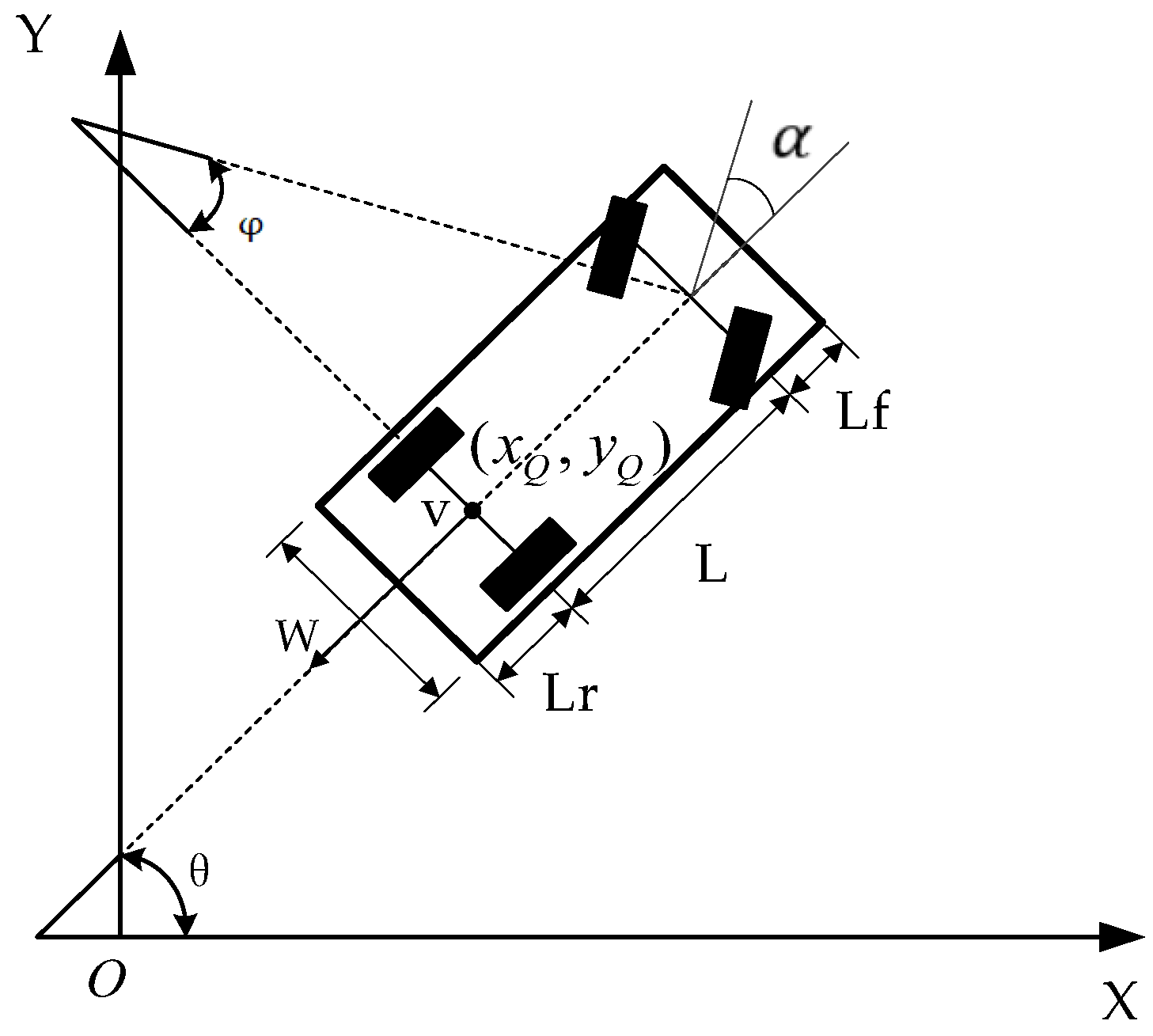
During the automatic parking process, a vehicle maintains a relatively low speed, typically around 2 km/h, and the lateral sliding generated during the parking process can be ignored [14]. The center of the vehicle’s rear axle is the base point, and the vehicle kinematics is modeled as shown in Figure 1.

By selecting the center of the equivalent vehicle rear axle as the reference point, because the speed of the whole parking process is less than 5 km/h, it can be assumed that the vehicle’s tires do not slide sideways during the parking process. The following differential equation can be obtained according to Figure 1.

$${\dot{x}}_{Q}sin\theta -{\dot{y}}_{Q}cos\theta =0$$

(1)

The kinematics equation of the center point of the equivalent rear axle can be obtained from Equation (1) and expressed as follows.

$$\left[\begin{array}{c}{\dot{x}}_Q\\ {\dot{y}}_Q\\ \dot{\theta }\end{array}\right]=\left[\begin{array}{c}cos\theta \\ sin\theta \\ tan\phi /L\end{array}\right]v$$

(2)

where $\theta$ represents the heading angle of the vehicle, $\alpha$ represents the Ackermann angle of the vehicle, which corresponds to the front wheel steering angle of the vehicle, $L$ represents the wheelbase of the vehicle, and $v$ represents the speed at the center point of the rear axle of the vehicle.

3. Automatic Parking Path-Planning Method

3.1. Narrow Parking Spaces

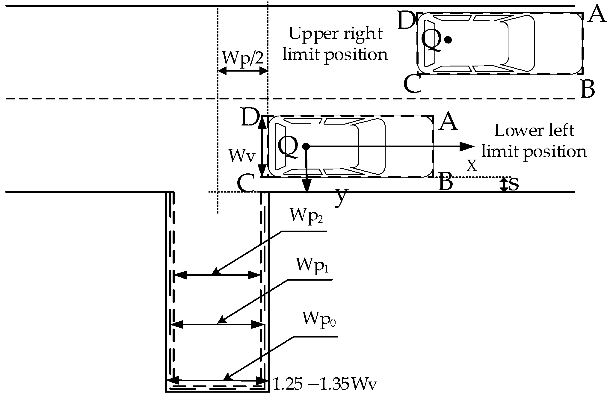
The size of a standard parking space is regulated by considering factors such as the width of the vehicle, the minimum turning radius of the vehicle, and parking safety. Let the width of the standard parking space be ${\mathrm{W}}_{{\mathrm{P}}_0}$. Generally, any parking space narrower than ${\mathrm{W}}_{{\mathrm{P}}_0}$ can be classified as a narrow parking space. However, the degrees of narrowness affect parking path planning. If the width of the parking space, denoted as ${\mathrm{W}}_{\mathrm{P}}$, is slightly narrower than ${\mathrm{W}}_{{\mathrm{P}}_0}$, specifically within the range of ${\mathrm{W}}_{{\mathrm{P}}_1}\le {\mathrm{W}}_{\mathrm{P}}\le {\mathrm{W}}_{{\mathrm{P}}_0}$, as shown in Figure 2, the vehicle can be parked in one step using the arc–line combination parking algorithm. When the width of the parking space falls within the range of ${\mathrm{W}}_{{\mathrm{P}}_2}\le {\mathrm{W}}_{\mathrm{P}}\le {\mathrm{W}}_{{\mathrm{P}}_1}$, the vehicle cannot be parked in one step, and if ${\mathrm{W}}_{\mathrm{P}}\le {\mathrm{W}}_{{\mathrm{P}}_2}$, the vehicle cannot be parked at all. In this study, we only consider multi-step parking, where a narrow parking space is defined as ${\mathrm{W}}_{{\mathrm{P}}_2}\le {\mathrm{W}}_{\mathrm{P}}\le {\mathrm{W}}_{{\mathrm{P}}_1}$, which is approximately 1.25–1.35 times the width of the vehicle body, denoted as ${\mathrm{W}}_V$, namely, ${\mathrm{W}}_{{\mathrm{P}}_1}\approx 1.35{\mathrm{W}}_{\mathrm{V}}$ and ${\mathrm{W}}_{{\mathrm{P}}_2}\approx 1.25{\mathrm{W}}_{\mathrm{V}}$.

3.2. Principles of the Arc–Line Combination Planning Algorithm

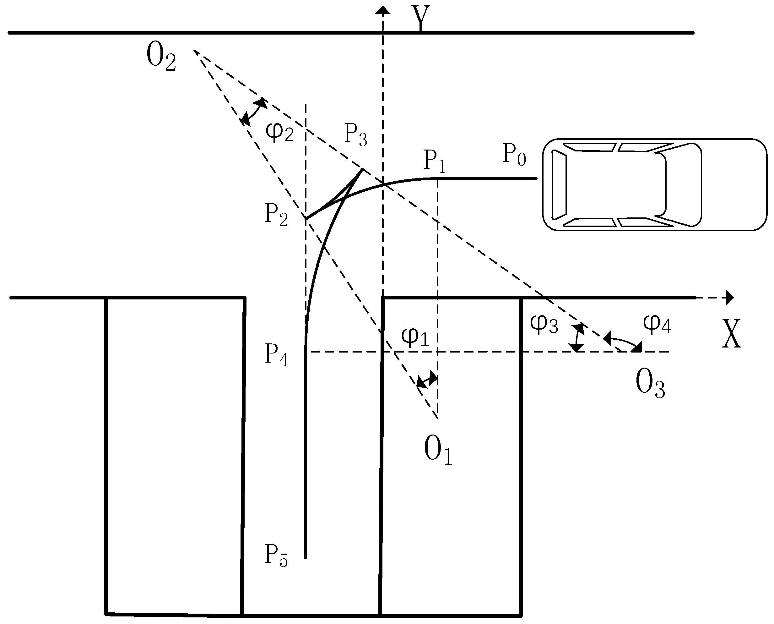
The arc–line combination vertical parking algorithm is a geometric algorithm, which is composed of multiple straight lines and arcs [15]. The radius of the arc corresponds to the minimum turning radius of the vehicle. An arc–line combination multi-step vertical parking path-planning diagram is shown in Figure 3. The parking path is composed of straight lines P₀P₁ and P₄P₅ as well as arcs P₁P₂, P₂P₃, and P₃P₄. The initial parking position is denoted as point P₀, while the final parking position is denoted as point P₅.

The first arc path is P₁P₂.

The vehicle reaches the initial parking position P₀ and starts parking within a safety threshold ψ; when the left rear of the vehicle and the left side of the parking space reach the safety threshold, the first arc P₁P₂ parking is completed.

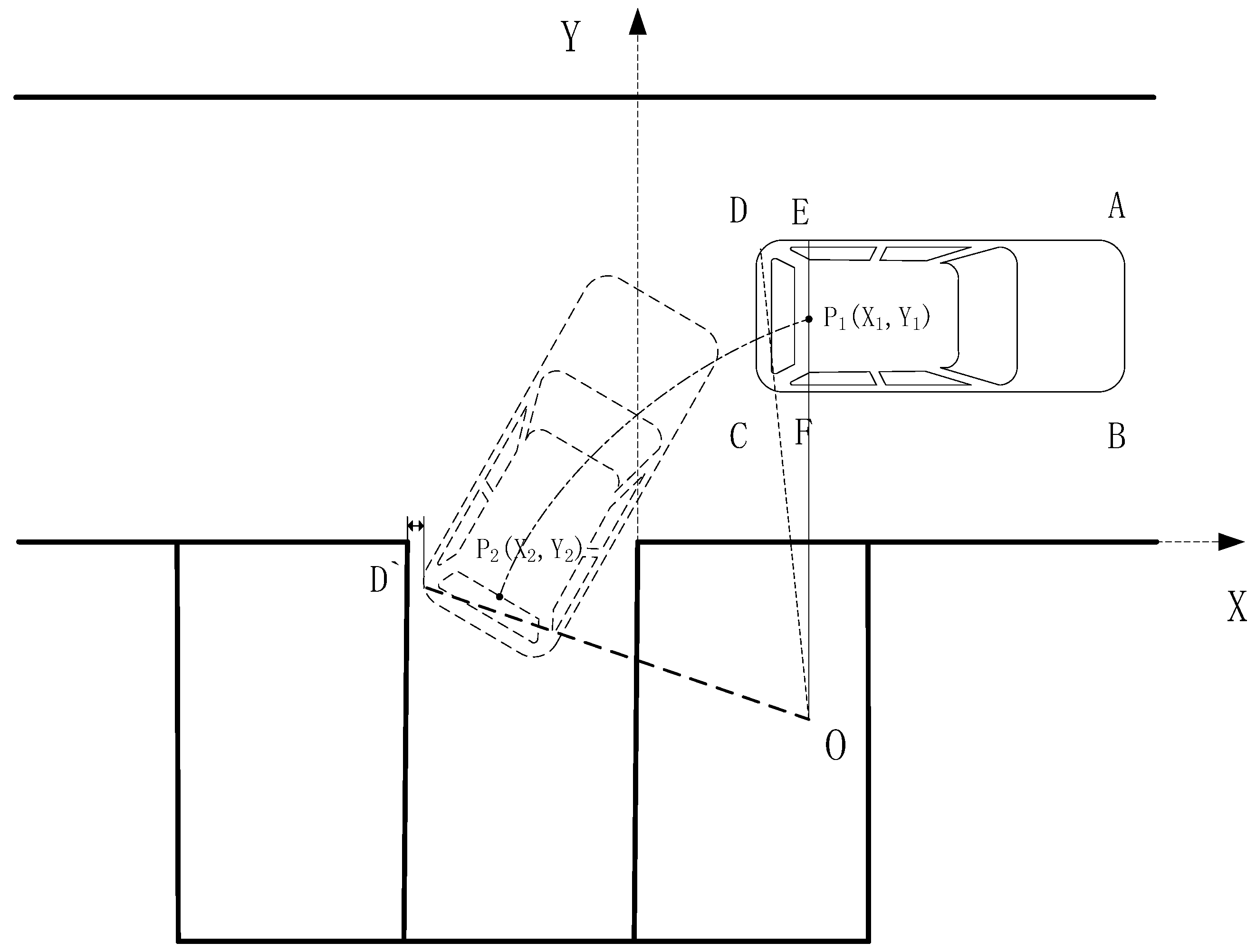
The arcs are obtained using their parameters. The angle parameter ${\phi }_0$, which represents the angle between the straight line OE and the straight line OD is obtained from Equation (3) and is shown in Figure 4.

$${\phi }_0=arctan\left(\frac{DE}{OE}\right)$$

(3)

The parameter corresponding to the first arc P₁P₂ is ${\phi }_1$. When the vehicle starts reversing from the initial parking position P₀, the left rear of the vehicle and the left side of the parking space reach the safety threshold. At this point, the left parking space vertex coordinates are denoted as D′ (X_D′, Y_D′). Based on the horizontal coordinate value of D’ and the rear axle center coordinate, the angle of the first arc (${\phi }_1$) can be determined.

$${\phi }_1=arcsin\left(\frac{X_1-X_{D\prime }}{OD}\right)-{\phi }_0$$

(4)

The second arc path is P₂P₃.

The parameters corresponding to the second arc path P₂P₃ are O₂ and ${\phi }_2$. The coordinates of the circle’s center O₂ (x_o2, y_o2) can be determined using the coordinates of the rear axle center Q₂ of the vehicle and the vehicle’s heading angle. The relationship between the center O₂ and center O₃ can be obtained from the geometric relationship between the tangent of the second and third arcs.

$${\left(x_{o3}-x_{o2}\right)}^2+{\left(y_{o3}-y_{o2}\right)}^2={\left(2R_{min}\right)}^2$$

(5)

The parameters corresponding to the third arc, P₃P₄, are O₃ and ${\phi }_3$. As the arc P₃P₄ is tangent to the straight line P₄P₅, the coordinates of O₃ (x_o3, y_o3) can be determined.

Based on the above analysis, the angle ${\phi }_2$ corresponding to the second arc path, P₂P₃, can be obtained.

$${\phi }_3=arctan\left(\frac{y_{o2}-y_{o3}}{x_{o3}-x_{o2}}\right)$$

(6)

$${\phi }_2=\frac{\pi }{2}-{\phi }_3-{\phi }_1$$

(7)

3.3. Principles of the Particle Swarm Optimization Planning Algorithm

The particle swarm optimization (PSO) algorithm is a random search algorithm known for its high precision, fast convergence speed, few parameters, and ease of implementation. With cooperation, the population is optimized. Each potential solution of an optimization problem is considered a bird in the search space, called a “particle” [16,17]. Each particle possesses a position determined with an objective function and a velocity that determines the flight distance and direction. All particles follow the current optimal particle to search in the solution space, aiming to find the optimal solution with multiple iterations.

Assuming an optimization problem is defined in a d-dimensional space, the number of particles in the population is $S_k$, and the position, velocity, and cost function values of the particles are ${X }_i=(x_{i1},x_{i2},\dots , x_{iD})$,$V_i=(v_{i1}, v_{i2},\dots , v_{iD})$, $f\left(X_i\right)$, respectively. The optimal particle within the population is denoted as $P_i$, which refers to the particle with the smallest cost function value of the current particle in all iterations. The global optimum is represented as $P_g$, which refers to the particle with the smallest cost function value among all optimal particles.

The velocity and position update formulas for the particles are as follows.

$$v_{id}\left(k+1\right)={\eta v}_{id}\left(k\right)+c_1{r}_1[P_{id}-x_{id}\left(k\right)]+c_2{r}_2[P_{gd}-x_{id}\left(k\right)]$$

(8)

$$x_{id}\left(k+1\right)=x_{id}\left(k\right)+v_{id}\left(k+1\right),1\le k\le k_{max},1\le i\le N_P,1\le d\le D$$

(9)

$$\eta \left(k\right)=\frac{\left({\eta }_{ini}-{\omega }_{end}\right)\left(k_{max}-k\right)}{k_{max}}+{\eta }_{end}$$

(10)

Among these formulas, $N_P$ represents the number of particles. Generally, a larger particle swarm size makes it easier to find the global optimal solution. $k_{max}$ denotes the maximum number of iterations. $v_{id}\left(k\right)$ represents the d-dimensional velocity component of the i-th particle in the k-th iteration, while $x_{id}\left(k\right)$ represents the d-dimensional position component of the i-th particle in the k-th iteration. $P_{id}$ represents the d-dimensional position component of the optimal particle $i$, and $P_{gd}$ represents the d-dimensional position component of the global optimum. The variables $r_1$ and $r_2$ are random functions that generate random numbers between 0 and 1. The parameter $\eta$ represents the inertia weight. Introducing an inertia weight provides the particle swarm with a more vital global search ability in the early stages and a more focused local optimization ability in the later stages. Increasing $\eta$ can improve the global search ability, while reducing $\eta$ can enhance the local search ability. Finding a reasonable value for $\eta$ is the key to achieving an efficient search and avoiding falling into local optima. The parameters $c_1$ and $c_2$ are acceleration coefficients that determine the weights for particle and global optimization guidance. $c_1$ affects the optimal local value, while $c_2$ affects the optimal global value.

PSO stop criterion: the end of the particle swarm optimization algorithm is either when the number of iterations reaches the maximum value or when the optimization result reaches the error threshold.

The PSO algorithm must find an optimal parking position and angle in vertical parking. Therefore, the position and angle of the vehicle are used as parameters of the objective function; specifically, the position and angle of the vehicle are used as the state vectors of the particles, and the objective function is the path function of arc straight line planning. By determining the independent variable that minimizes the objective function and the starting point of parking, the parking point position information of the parking point can obtained based on the vehicle’s minimum turning radius and the objective function’s minimum value. The objective function is used to evaluate the position, and with continuous attempts and adjustments, the algorithm searches for the optimal solution, resulting in a fast and efficient vertical parking process.

3.4. Principles of the Hybrid A* Planning Algorithm

The Hybrid A* algorithm differs from the traditional A* algorithm in several ways. It is a state-space heuristic algorithm that incorporates heuristic information during the search process. This algorithm is specifically designed for vehicle kinematics and is suitable for gridded parking environments. In the Hybrid A* algorithm, each location in the gridded state space is evaluated to determine the best position. From this position, a subsequent search is performed toward the destination. This approach ensures that the search path adheres to the vehicle’s kinematics and allows for efficient navigation in the parking environment [18,19,20].

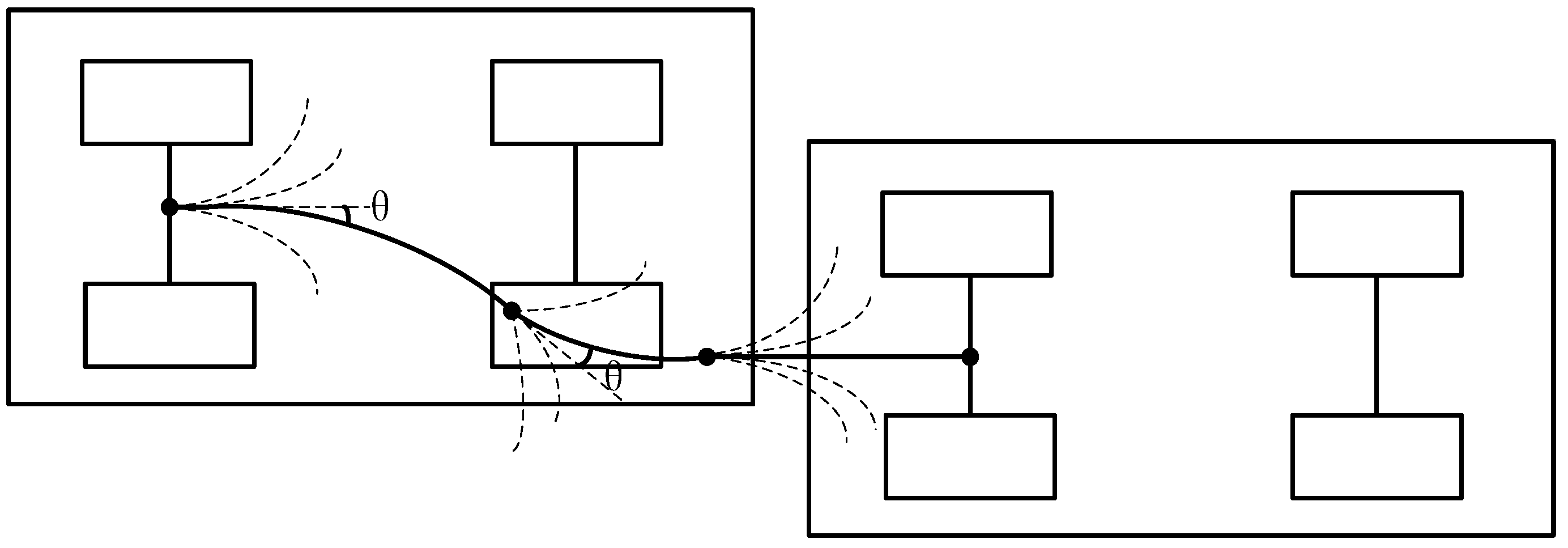
The Hybrid A* algorithm is commonly used in various path-planning applications, including automatic parking path planning [21]. It extends from the parent node with various steering operations (left turn, right turn, or no turn), and combines the vehicle kinematics model to determine new nodes, ensuring the continuity of motion between the child node and the parent node. As a result, the path generated using the Hybrid A* algorithm satisfies the requirements of vehicle driving, as shown in Figure 5.

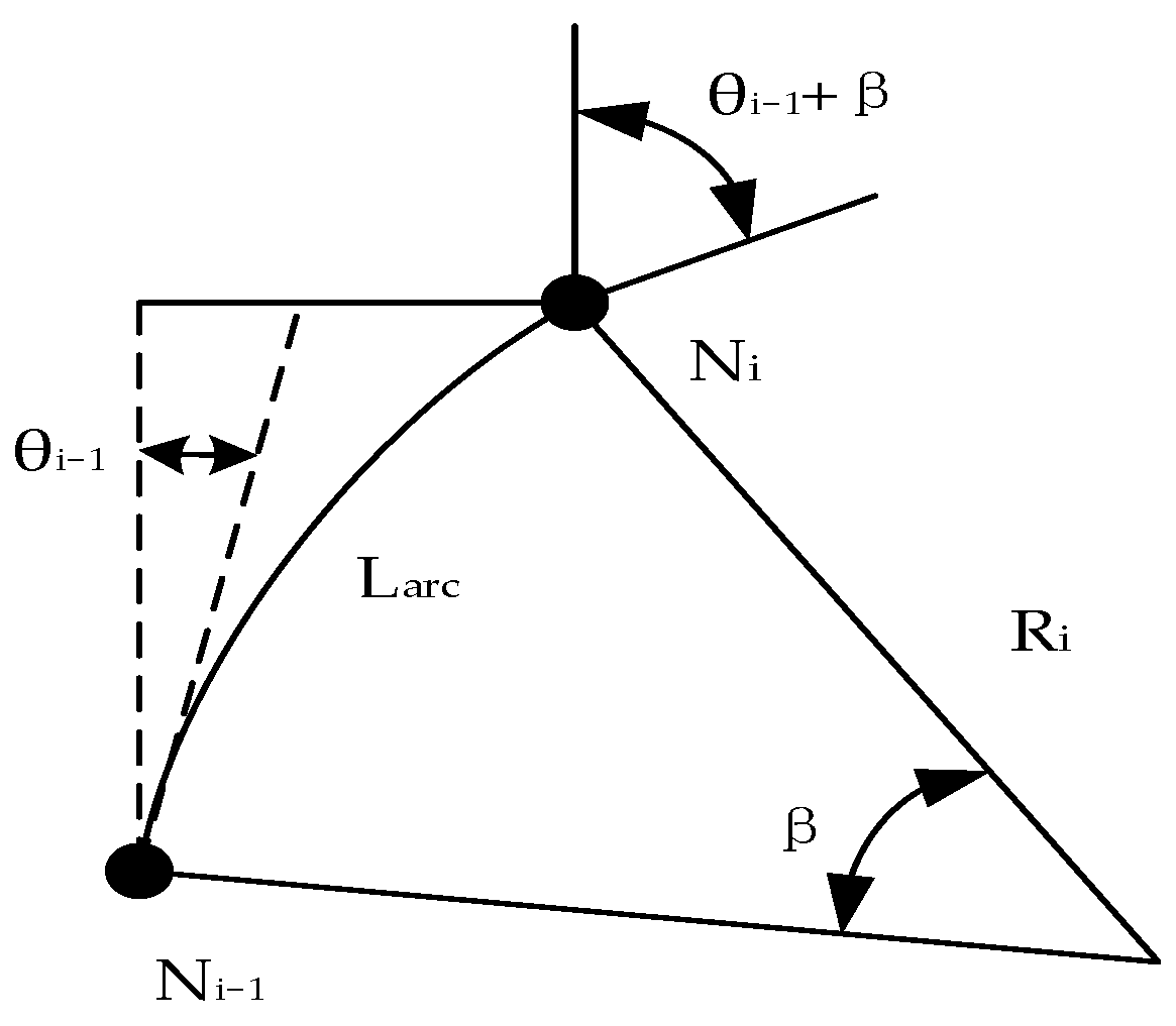
In path planning, three-dimensional coordinates $(x, y, \theta )$ describe the vehicle’s posture. Where $x$ represents the horizontal coordinate, $y$ represents the vertical coordinate, and $\theta$ represents the heading angle of the vehicle. The node expansion process of the Hybrid A* algorithm is shown in Figure 6. In this process, $N_{i-1}$ and $N_i$ represent the previous node and the current node, respectively. The basic principles of the algorithm are shown in Equations (11)–(15).

$$\beta =\left(\frac{L_{arc}}{W_v}\right)\times tan\alpha$$

(11)

$$R_i=\frac{L_{arc}}{\beta }$$

(12)

$$x_i=x_{i-1}+R_i\left[sin\right({\theta }_{i-1}+\beta )-sin({\theta }_{i-1}\left)\right]$$

(13)

$$y_i=y_{i-1}-R_i\left[cos\right({\theta }_{i-1}+\beta )+cos({\theta }_{i-1}\left)\right]$$

(14)

$${\theta }_i={\theta }_{i-1}+\beta$$

(15)

where $L_{arc}$ represents the step size of each extension of the Hybrid A* algorithm, $\alpha$ represents the steering angle of the vehicle, and $W_v$ represents the track width. The angle of $\beta ,$ corresponding to the arc between the $N_{i-1}$ and $N_i$ nodes, can also be directly set as the minimum turning radius of the vehicle during the expansion process.

The Hybrid A* algorithm considers the influence of the front wheel angle on node expansion, resulting in a three-dimensional coordinate representation $(x, y, \theta )$. At the same time, two heuristic functions are considered: the unconstrained heuristic function and the constrained heuristic function. Among them, the unconstrained heuristic function ignores the non-holonomic constraints of the vehicle and considers the environmental obstacles. Therefore, it is not necessary to consider the kinematic constraints of the vehicle, such as the heading angle. On the other hand, the constrained heuristic function ignores environmental obstacles and considers vehicle non-integrity constraints. The unconstrained heuristic function value is used to calculate the constrained heuristic function value, and the Reeds–Shepp curve is used to calculate the size of the heuristic function value.

3.5. The Parking Path Evaluation Function

The planned path length is commonly used as an indicator to measure the performance of standard spaces parking. However, it is not suitable for evaluating narrow-space parking due to the frequent changes in speed and direction. In this paper, we propose a multi-objective evaluation function for narrow parking space paths to evaluate the comprehensive performance of parking algorithms.

1.

The number of positive and negative transitions in vehicle speed, denoted as R, can be determined by examining the speed direction at previous and subsequent moments. Positive transitions occur when the vehicle speed changes from a lower value to a higher value, while negative transitions occur when the vehicle speed changes from a higher value to a lower value. By analyzing these transitions, we can gain insights into the dynamics and changes in the vehicle’s speed during the parking process.

2.

The total length of the path.

$$L={\sum }_{i=1}^N{\left({\left(x\left(i+1\right)-x\left(i\right)\right)}^2+{\left(y\left(i+1\right)-y\left(i\right)\right)}^2\right)}^{\frac{1}{2}}$$

(16)

3.

Path Smoothness.

The minimum curvature of the path curve can represent the smoothness of the path curve. The smaller the minimum curvature, the better the smoothness of the path curve. The average minimum curvature of the entire parking path curve can be compared.

$$\overline{\rho }=mean\left({\rho }_{i1min},{\rho }_{i2min},{\rho }_{i3min}\right)$$

(17)

where ${\rho }_{i1min}$ represents the minimum curvature of the first path curve of the i-th path point; ${\rho }_{i2min}$ represents the minimum curvature of the second segment of the curve at the i-th path point; and ${\rho }_{i3min}$ represents the minimum curvature of the third segment of the curve at the i-th path point.

The multi-objective evaluation function value, denoted as S, for the planning path of these three planning algorithms is obtained by separately calculating the values of the above three evaluation indicators and then performing a weighted summation. The specific calculation of S depends on the weights assigned to each evaluation indicator. By combining the individual indicator values with their respective weights, the multi-objective evaluation function provides a comprehensive assessment of the planning path, as follows.

$$S={\omega }_{l}L+{\omega }_{r}R+{\omega }_{\rho }\overline{\rho }$$

(18)

where ${\omega }_l$ represents the weighted coefficient of the total path length; ${\omega }_r$ represents the weighted coefficient of the number of positive and negative conversions of vehicle speed; and ${\omega }_{\rho }$ represents the weighted coefficient of the planned path curvature.

4. Path-Planning Simulation

4.1. Parking Scene Settings

According to the “Specification for the Setting of Parking Spaces on Urban Roads,” (GA/T 850—2021 of China) the width of vertical parking spaces for small cars is 2.5–2.7 m. The width of the single-lane turning lane is not less than 3.5 m, while the width of the double lane is not less than 5 m. The turning section should meet the needs of one vehicle turning at a time. This paper selects a small sedan as the research object, with a width of 1.737 m, a length of 4.579 m, a minimum turning radius of 5.6 m, and a safety threshold between vehicle and parking space, ψ, ψ = 0.1 m. According to the above definition of narrow parking spaces, this paper sets the parameters for narrow parking spaces as shown in

Table 1. Parameters of narrow parking scenarios.

Scene Parameters	Parking Space Width SW/m	Parking Space Length SL/m	Length of Driving Passage L/m	Width of Driving Passage W/m	Vehicle’s Initial Heading Angle θmin/(°)
Value	2.3~2.1	5.0	9.0	5.0	−10~10

.

4.2. Simulation

To select a more suitable parking planning algorithm for narrow parking spaces, the arc–line combination, Hybrid A*, and particle swarm optimization algorithms are modeled and a narrow parking scene is established in MATLAB. Then, with the given starting point and different parking space widths, the three algorithms are used to generate different planned paths. The path length, the number of positive and negative conversions of vehicle speed, and the curvature are obtained to compare the performance of the algorithms based on the multi-objective function. The values obtained from the multi-objective function indicate the fitness of each algorithm in the narrow parking environment.

The following is a comparison of the paths planned with the three algorithms when the parking space width is a standard size of 2.5 m, as shown in Figure 7.

It can be seen that the path planned using the Hybrid A* algorithm consists of two arcs and a straight line, whereas the path planned with the arc–line combination and particle swarm optimization includes three arcs and a straight line. Moreover, the first arc in the Hybrid A* planning is significantly smaller compared with the arc–line combination and particle swarm optimization. As a result, to complete the parking operation, the path of the Hybrid A* planning needs to be adjusted once outside the parking space to enter it, while the arc straight line and the particle swarm optimization paths need to be adjusted twice outside the parking space. In the following simulation, we will compare the widths of different parking spaces.

The path curve can be discretized into numerous path points, each containing $(x, y)$ coordinate values. Subsequently, according to the path length calculation formula in the parking path evaluation indicator in Section 3.5, the arc–line combination, Hybrid A*, and particle swarm optimization path lengths can be calculated. Based on each coordinate point, the curvature calculation formula can be used to obtain the curvature value corresponding to each arc segment.

4.2.1. The Arc–Line Combination

The path length and curvature for the arc–line combination planning algorithm were simulated using MATLAB for various parking space widths. The results of the simulation are presented below.

The curvature diagram below illustrates the simulated path using the arc–line planning algorithm in three narrow parking spaces with varying widths. Although the parking spaces have different widths, the curvature mutations remain consistent. From Figure 8, the curvature of the first arc has two mutation points, the second arc has two mutation points, and the third arc has two mutation points. The comparison information of path length and reverse times simulated using MATLAB for different parking space widths can be seen in

Table 2. Planned paths of the arc–line combination algorithm for different parking spaces.

Evaluation Indicators	Values
	${\mathbf{W}}_{\mathbf{p}}$ = 2.3	${\mathbf{W}}_{\mathbf{p}}$ = 2.2	${\mathbf{W}}_{\mathbf{p}}$ = 2.1
Total path length/m	11.39	11.37	11.21
Positive and negative speed conversion times/time	2	2	2
Distance between vehicle and parking space/m	0.2	0.1	0.09
Planned path

.

4.2.2. Hybrid A*

The path length and curvature of the Hybrid A* planning algorithm were simulated using MATLAB for various parking space widths. The results of the simulation are presented below.

The diagram below illustrates the curvature map of the simulated path using the Hybrid A* planning algorithm in three narrow parking spaces with varying widths. Although the parking spaces have varying widths, the curvature mutations remain consistent. From Figure 9, the curvature of the first arc has two mutation points, the second arc has two mutation points, and the third arc has two mutation points. The comparison information of path length and reverse times simulated using MATLAB for different parking space widths can be seen in

Table 3. Planned paths of the Hybrid A* algorithm for different parking spaces.

Evaluation Indicators	Values
	${\mathit{W}}_{\mathit{p}}$ = 2.3	${\mathit{W}}_{\mathit{p}}$ = 2.2	${\mathit{W}}_{\mathit{p}}$ = 2.1
Total path length/m	9.48	9.50	9.53
Positive and negative speed conversion times/time	2	2	2
Distance between vehicle and parking space/m	0.2	0.1	0.09
Planned path

.

4.2.3. Particle Swarm Optimization

The particle swarm parameters are set based on practical engineering experience to ensure reasonable optimization. The path length and curvature of the particle swarm optimization algorithm were simulated using MATLAB for different parking space widths. The results are presented below.

The diagram below illustrates the curvature of the simulation path using the particle swarm optimization algorithm in narrow parking spaces. From Figure 10, the curvature of the first arc has two mutation points, the second arc has two mutation points, and the third arc has two mutation points. The curvature map planned with the particle swarm optimization algorithm is similar to the arc–line planning algorithm. However, the segmented arcs in Figure 10 exhibit faster changes in curvature compared with the arc–line combination algorithm, resulting in a less smooth curvature profile. Additionally, the second mutation in the third arc appears to be more severe than the mutation in the straight arc. The comparison information of path length and reverse times simulated using MATLAB for different parking space widths can be seen in

Table 4. Planned paths of the particle swarm optimization algorithm for different parking spaces.

Evaluation Indicators	Values
	${\mathbf{W}}_{\mathbf{p}}$ = 2.3	${\mathbf{W}}_{\mathbf{p}}$ = 2.2	${\mathbf{W}}_{\mathbf{p}}$ = 2.1
Total path length/m	9.47	9.48	9.50
Positive and negative speed conversion times/time	2	2	2
Distance between vehicle and parking space/m	0.1	0.09	0.08
Planned path

.

Based on the above simulation results, it can be found that the path needs to be adjusted multiple times to park smoothly due to the narrow space, regardless of whether the arc–line combination, Hybrid A*, or particle swarm optimization algorithms are used. From the three tables, it can be observed that the path planned with the arc–line combination algorithm has the longest length. Additionally, the three planning algorithms exhibit the same number of positive and negative vehicle speed conversions, indicating an equal number of reverse times. Analyzing the path length, the number of positive and negative vehicle speed transitions, and the number of vehicle position adjustments outside the depot in Figure 7, it can be concluded that the parking operation time of the path planned with the geometric algorithm is relatively long, and the efficiency is relatively low.

By analyzing the paths in Figure 7 and the information provided in the tables, it can be found that the Y values of the adjusted coordinates for the arc–line combination and particle swarm optimization planning paths outside the garage are relatively large. This indicates that the vehicle’s position is farther away from the garage compared with the Hybrid A* algorithm. Considering that the width of the driving lane is 5 m, being further away from the garage increases the risk of a vehicle coming into contact with the curb, opposite vehicles, or walls, which can result in parking failure.

The simulation results demonstrate that the Hybrid A* algorithm is particularly suitable for narrow parking spaces. It successfully parks a vehicle in a parking space with a width of 2.1 m, while both the arc–line combination and Hybrid A* algorithms achieve parking successfully at a width of 2.2 m. Furthermore, all three algorithms successfully park the vehicle in parking spaces with a width of 2.3 m. This indicates that the Hybrid A* algorithm is most suitable when dealing with a relatively narrow parking environment.

Based on the multi-objective evaluation function, a comparison of the results from three parking planning algorithms is presented in

Table 5. Performance of the three algorithms.

Algorithm	Total Path Length/m	Positive and Negative Speed Conversion Times/Time	$\overline{\mathit{\rho }}$	S
Arc–line combination	11.39	2	0.159	79.84
Hybrid A*	9.48	2	0.151	74.25
PSO	9.47	2	0.161	78.24

.

Based on comprehensive analysis, it can be observed that the arc–line combination planning algorithm has the longest path among the three evaluation indicators, while the particle swarm optimization has the shortest path. The number of positive and negative vehicle speed transitions is the same for all three algorithms. In terms of curvature, the Hybrid A* algorithm exhibits the smallest average minimum curvature among the three arcs, while the particle swarm optimization algorithm has the largest curvature. When considering the final evaluation function S, the Hybrid A* algorithm has the lowest score, indicating its suitability for narrow parking spaces. On the other hand, the arc–line combination algorithm has the highest score, significantly differing from the other two other planning algorithms. This suggests that the arc–line combination algorithm is not suitable for narrow parking spaces. Although the particle swarm optimization algorithm has the same evaluation score as Hybrid A* for a 2.3 m wide parking space and the shortest path, it is important to note that the path is not as smooth as the Hybrid A* algorithm and exhibits more significant curvature mutations. Therefore, the Hybrid A * algorithm is considered more suitable for narrow parking spaces.

Although the Hybrid A* algorithm is better overall, it also has the issue of curvature discontinuity in the path curve, leading to a spot turn. In order to solve the problem of curvature discontinuity of the planned path, it is necessary to incorporate path-smoothing techniques into the optimization process to ensure a more continuous and smoother path.

5. Path-Smoothing Optimization of the B-Spline Curve and Gradient Descent Algorithm

Gradient descent is a numerical optimization algorithm known for its small storage capacity and high stability. The gradient of the function (the tangent slope of the function at this point) can effectively determine the direction in which the function value decreases the fastest; this iterative process allows the algorithm to approach the optimal solution step by step [22,23]. The gradient descent algorithm can optimize the curvature of the smoother curve and adjust the curvature of the curve to meet the kinematic requirements of vehicle driving. However, it is important to note that if the curve is not smooth in certain areas, there may be no gradient available, rendering the gradient descent algorithm unable to optimize in those specific places.

The optimization of parking paths in narrow spaces involves selecting a series of control points, including the starting and ending points of the curve. To address the limitations of the gradient descent algorithm in handling non-smooth paths, the B-spline curve is utilized for path smoothing. The B-spline curve is known for its multi-order derivative continuity, which ensures a smooth and continuous path. In the case of narrow parking spaces, the parking paths consist of multiple segments of arcs and straight lines. To optimize each arc in the multi-step parking process, B-spline curves are used. By utilizing the optimized smooth curve, the gradient descent algorithm can effectively optimize the path curvature and ensure a smoother parking path.

5.1. Path Smoothing Optimization Based on the B-Spline Curve

The B-spline curve is an improved curve based on the Bézier curve [24]. It can not only change the order of the curve but also realize the local change in the curve. Assuming that there are $n$ control vertices, the k-order B-spline curve function is expressed as follows.

$$P\left(u\right)={\sum }_{i=0}^n{P}_i{N}_{i,k}\left(u\right)$$

(19)

In the above formula, $k=\{ 0, 1, 2,\dots , n \}$ and $U=\{ u_0,{ u}_1, \cdots , u_{(n+k+1)} \}$ represents the node vector sequence. $P_i$ denotes the ith curve equation corresponding to the i-th point, and $N_{(i, k)}\left(u\right)$ is the k-th B-spline basis function. The recurrence formula is as follows.

$$\left\{\begin{array}{c}define\frac{0}{0}=0 \\ N_{i,0}\left(u\right)=\left\{\begin{array}{c}1, u_i\ll u\ll u_{i+1}\\ 0, other \end{array}\right. \\ N_{i,k}\left(u\right)=\frac{(u-u_i)N_{i,k-1}\left(u\right)}{u_{i+k}-u_i}+\frac{{(u}_{i+k+1}-u)N_{i+1,k-1}\left(u\right)}{u_{i+k+1}-u_{i+1}}, u_k\le u\le u_{n+1}\end{array}\right.$$

(20)

According to the structure of the B-spline curve, its shape is determined by the node vector and the control point of the piecewise mixed function. Then, according to the distribution of the midpoint of the node vector sequence U, the B-spline curve can be classified into four types [25]: uniform B-spline curve, quasi-uniform B-spline curve, piecewise Bézier curve, and non-uniform B-spline curve.

When optimizing the parking path, the starting point and the endpoint of parking cannot be ignored. The quasi-uniform B-spline curve is selected in this paper as it satisfies the requirements of passing through the starting points and endpoints. This curve closely resembles the original trajectory, allowing for the preservation of the original path’s shape to the maximum extent. Therefore, this paper chooses this curve to optimize the parking path. In the case where the value of $k$ in Equation (21) is 3, the expression for the cubic quasi-uniform B-spline can be obtained.

$$P\left(u\right)={\sum }_{i=0}^3{P}_i{N}_{i,k}\left(u\right)$$

(21)

Then, this paper uses the B-spline curve to fit each path arc to obtain a smooth path. The specific algorithm process is as follows: first, path planning is carried out to obtain the path point set, and the opposite change position of the vehicle movement direction is judged. Then, multiple arc path curves are obtained by segmenting the complete path, and B-spline curves are used to optimize each path curve. Finally, the final smooth path is obtained by stitching the optimized path curves.

5.2. Path Curvature Optimization Based on Gradient Descent

To ensure that the curvature of the optimized path, denoted as $X_i=(x_i,{ y}_i)$, $i\in [ i, N ]$, satisfies the minimum turning radius constraint of the vehicle, an objective function is designed for re-optimization. The goal is to control the planned path curvature so that it does not exceed the maximum turning curvature of the vehicle.

$$F={\omega }_c{\sum }_{i=1}^{N-1}{\sigma }_c\left(\frac{∆{\varnothing }_i}{\left|∆X_i\right|}-k_{max}\right)$$

(22)

where ${\varnothing }_i$ represents the change in tangential angle at the vertex, ${\omega }_c$ represents the weight of the curvature term, ${\sigma }_c$ is the penalty function, $∆X_i=X_i-X_{i-1}$ is the displacement at point $X_i$, and $∆{\varnothing }_i$ represents the angle change in the path at the point $X_i$. Additionally, $k_{max}$ represents the maximum curvature of the vehicle during turning; among them,

$$∆{\varnothing }_i=\left|{tan}^{-1}\left(\frac{∆y_{i+1}}{∆x_{i+1}}\right)+{tan}^{-1}\left(\frac{∆y_i}{∆x_i}\right)\right|$$

(23)

The curvature is affected by the derivative of the three points $X_i$, $X_{i+1}$, and $X_{i-1}$ and the curvature $k_i=\frac{∆{\varnothing }_i}{\left|∆X_i\right|}$; therefore,

$$∆{\varnothing }_i={cos}^{-1}\left(\frac{∆X_i^T∆X_{i+1}}{\left|X_i^T\right|\left|∆X_{i+1}\right|}\right)$$

(24)

The partial derivatives of curvature to $X_i$, $X_{i+1}$, and $X_{i-1}$ are calculated, respectively, and the following results are obtained.

$$\frac{\partial k_i}{\partial X_i}=-\frac{1}{\left|∆X_i\right|}\frac{\partial ∆{\varnothing }_i}{\partial cos\left(∆{\varnothing }_i\right)}\frac{\partial cos\left(∆{\varnothing }_i\right)}{\partial X_i}-\frac{\partial ∆{\varnothing }_i}{∆X_i^2}\frac{\partial ∆X_i}{\partial X_i}$$

(25)

$$\frac{\partial k_i}{\partial X_{i+1}}=-\frac{1}{\left|∆X_i\right|}\frac{\partial ∆{\varnothing }_i}{\partial cos\left(∆{\varnothing }_i\right)}\frac{\partial cos\left(∆{\varnothing }_i\right)}{\partial X_{i+1}}$$

(26)

$$\frac{\partial k_i}{\partial X_{i-1}}=-\frac{1}{\left|∆X_i\right|}\frac{\partial ∆{\varnothing }_i}{\partial cos\left(∆{\varnothing }_i\right)}\frac{\partial cos\left(∆{\varnothing }_i\right)}{\partial X_{i-1}}-\frac{\partial ∆{\varnothing }_i}{∆X_i^2}\frac{\partial ∆X_i}{\partial X_{i-1}}$$

(27)

The gradient formula of curvature is

$$\frac{\partial F}{\partial X_i}={\omega }_c\left({\omega }_{i-1}\frac{\partial k_i}{\partial X_{i-1}}+{\omega }_i\frac{\partial k_i}{\partial X_i}+{\omega }_{i+1}\frac{\partial k_i}{\partial X_{i+1}}\right)$$

(28)

For Equations (25)–(27), according to the curvature gradient formula, the following can be obtained

$$\frac{\partial ∆{\varnothing }_i}{\partial cos}=\frac{\partial {cos}^{-1}\left(cos\left(∆{\varnothing }_i\right)\right)}{\partial cos\left(∆{\varnothing }_i\right)}=\frac{-1}{{\left(1-{cos}^2\left(∆{\varnothing }_i\right)\right)}^{1/2}}$$

(29)

In summary, the algorithm calculates curvature penalty term for each path point based on the current path sequence. These curvature terms are weighted and summed to form the overall objective function. In each iteration, the coordinate correction value for each point on the path is obtained using gradient derivation of the objective function. Then, the original coordinate values of each point are adjusted by adding the correction value, resulting in a new path optimized through one iteration of gradient descent. The algorithm continues this process for a set total number of iterations, M, until convergence to the final optimized path is achieved.

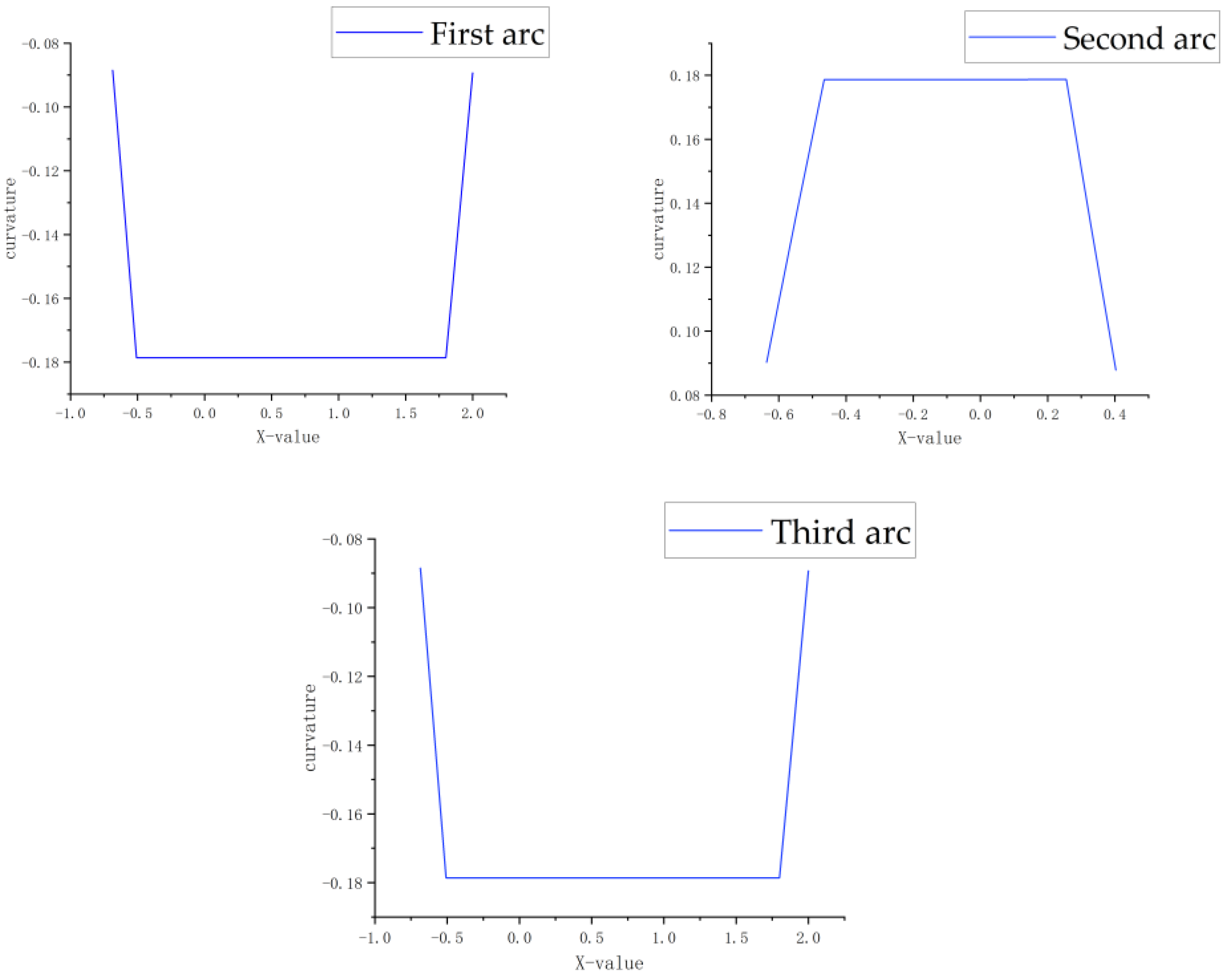
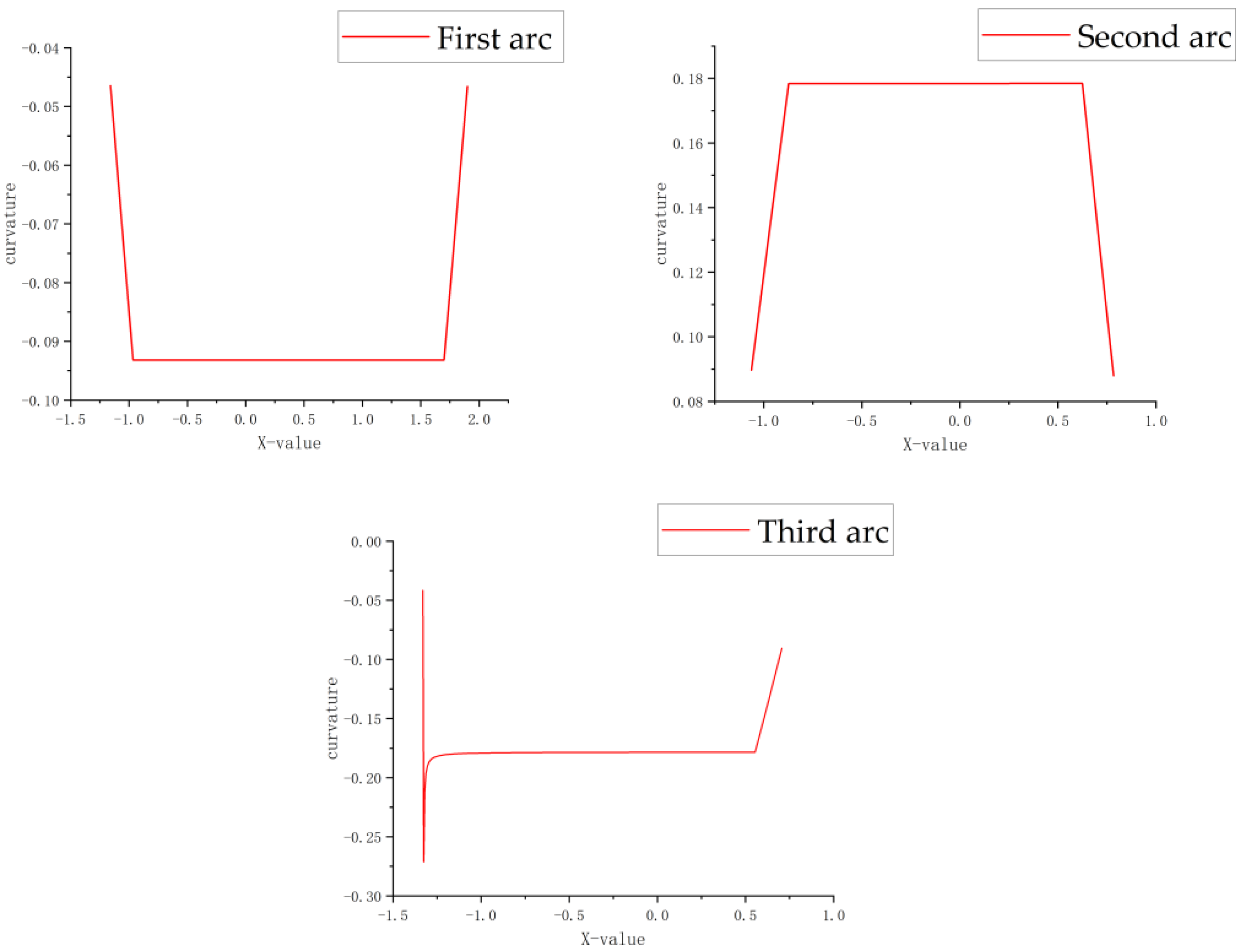
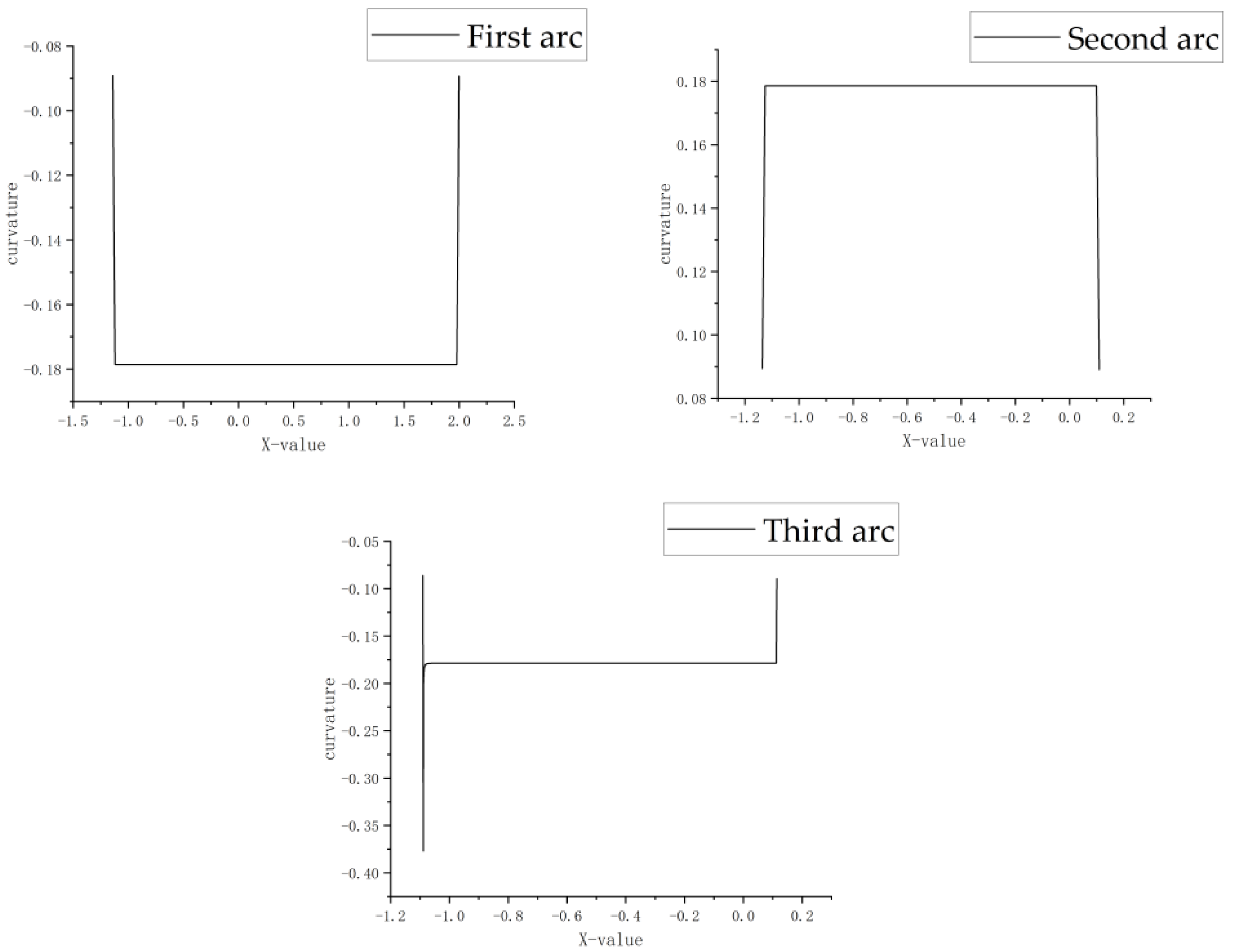
According to the same path information of the Hybrid A* algorithm in Section 4.2 and the MATLAB simulation, the following figure shows the curvature comparison after Hybrid A* path optimization.

Figure 11a shows a comparison of the curvature for the first arc parking path of the Hybrid A* algorithm before and after applying the B-spline curve and the gradient descent algorithm. Similarly, Figure 11b compares the curvature for the second arc parking path, and Figure 11c compares the curvature for the third arc parking path. In Figure 11a,b, the mean curvature becomes smaller after applying the B-spline curve and the gradient descent algorithm. Although the curvature in Figure 11c becomes more significant, the curvature of all three path curves remains continuous without mutation. This ensures that the curvature change in parking path planning is continuous and satisfies the minimum turning radius constraint of the vehicle.

The Hybrid A* path curve with a width of 2.3 m and the optimized path curve of 3.2 parking spaces are selected. The multi-objective evaluation function compares the multi-objective function S values before and after optimization. The simulation results can be seen in

Table 6. Performance comparison between optimized Hybrid A* algorithm and the other algorithms.

Algorithm	Total Path Length/m	Positive and Negative Speed Conversion Times/Time	$\overline{{\mathit{\rho }}_{\mathit{i}}}$	S
Hybrid A* (without optimization)	9.48	2	0.151	74.25
Hybrid A* (optimization)	10.02	2	0.146	74.18
PSO	9.47	2	0.161	78.24
Arc–line combination	11.39	2	0.159	79.84

.

For a narrow space parking, the vehicle needs frequent small steering, which results in large path curvature and impacts the parking safety significantly; therefore, it should be given the maximum weight. It can be seen from the simulation results that the number of positive and negative conversions of the vehicle speed is the same in the narrow parking environment. Therefore, the path curvature, the path length, and the number of positive and negative conversions are weighted as 70%, 20%, and 10%, respectively. The three evaluation indicator values are normalized using the scale transformation method shown in (30).

$$X_L=\frac{X_{L_{min}}}{X_{L_i}}, X_R=\frac{X_{R_{min}}}{X_{R_i}}, X_{\rho }=\frac{X_{{\rho }_{min}}}{X_{{\rho }_i}}$$

(30)

Based on the comprehensive analysis, the curvature of the Hybrid A* path is effectively optimized using the B-spline curve and the gradient descent algorithm. The average value of the minimum curvature was reduced by 0.005 m⁻¹ compared with the curvature before optimization. This value is also lower than the curvature of the arc–line combination and the particle swarm optimization algorithm. Although the optimized Hybrid A* algorithm results in a slightly longer path length, with an increase of 1.54 m, the function value after optimization is reduced by 0.07. As shown in

Table 7. Normalized performance comparison between the optimized Hybrid A* algorithm and the other algorithms.

Algorithm	${\mathit{X}}_{\mathit{L}}$/m	${\mathit{X}}_{\mathit{R}}$/Time	${\mathit{X}}_{\mathit{\rho }}$	S
Hybrid A* (without optimization)	0.999	1	0.967	0.887
Hybrid A* (optimization)	0.945	1	1	0.899
PSO	1	1	0.907	0.845
Arc–line combination	0.831	1	0.918	0.819

, after the three evaluation indicator values are normalized, the multi-objective evaluation function value of the Hybrid A* algorithm is the largest. This finding indicates that the optimized Hybrid A* algorithm is more suitable for a narrow parking environment, aligning with the results presented in Table 6.

The simulation results show that in the narrow parking environment, the path of the Hybrid A* algorithm optimized with the B-spline curve and the gradient descent algorithm proposed in this paper is better overall. Compared with the Hybrid A* algorithm, the proposed algorithm can further improve the smoothness of the planned path. Compared with the arc–line combination, it can generate a trajectory with a smooth path and speed. Compared with the particle swarm optimization algorithm, the actual motion constraints of the object are considered, which makes it generate a more realistic path. However, the Reed–Shepp curve is used in the proposed algorithm for path generation, which leads to a higher calculation load.

6. Conclusions

This paper introduces the concept of a narrow parking space and provides a definition based on the standard when the arc–line combination parking algorithm fails to park the vehicle in a single step. The parking space is defined as a narrow parking space when the width of the parking space is approximately 1.25–1.35 times the width of the vehicle body, denoted as ${\mathrm{W}}_{{\mathrm{P}}_1}\approx 1.35{\mathrm{W}}_{\mathrm{P}}$ and ${\mathrm{W}}_{{\mathrm{P}}_2}\approx 1.25{\mathrm{W}}_{\mathrm{P}}$. Aiming at the narrow parking space and narrow parking environment, a multi-objective function is proposed to evaluate the applicability of three planning algorithms, namely, the arc straight–line, Hybrid A*, and particle swarm optimization algorithms, in a narrow parking space.

The curvature of the parking path curve is discontinuous, and severe mutations result in spot turns according to the simulation results and the analysis of narrow parking environments. This paper proposes an algorithm based on the B-spline curve and gradient descent algorithm to optimize the path to solve the problem of discontinuous and abrupt curvature of the path curve. The optimized path curvature is smooth and satisfies the minimum turning radius constraint of the vehicle.

However, certain aspects such as speed planning, parking space detection and recognition, and parking path following control are not considered in this paper. In the future, variable speed planning and the recognition of narrow parking spaces by vehicles and the following control of vehicles will be considered.