RepRCNN: A Structural Reparameterisation Convolutional Neural Network Object Detection Algorithm Based on Branch Matching

Abstract

A CNN object detection method based on the structural reparameterisation technique using branch matching is proposed to address the problem of balancing accuracy and speed in object detection techniques. By the structural reparameterisation of the convolutional layer in the object detection network, the amount of computation and the number of parameters in the network inference are reduced, the memory overhead is lowered, and the use of the branch-matching method to improve the structural reparameterisation model improves the computational efficiency and speed of the network while maintaining the detection accuracy. Optimisation is also carried out in terms of target screening and loss function, and a new CPC NMS screening strategy was introduced to further improve the performance of the model. The experimental results show that the proposed method achieves competitive results on the PASCAL VOC2012 and MS COCO2017 datasets compared to the traditional object detection methods and the current mainstream models, achieving a better balance between the detection accuracy and detection speed.

1. Introduction

Object detection is an important branch in the field of computer vision, and its main task is to identify the location and category of the target from the image. In recent years, with the rapid development of deep learning technology in the field of computer vision, the field of object detection has also made great progress, and deep learning-based object detection algorithms have become the mainstream method. Object detection can currently be divided into one-stage detection and two-stage detection methods. One-stage detection models such as YOLO [1] and SSD [2] have a fast detection speed but slightly lower accuracy, and the models in the YOLO series [1,3,4] have achieved the recognition of researchers; two-stage detection methods such as the faster R-CNN [5] model have a clear advantage in terms of their accuracy in object detection, but it is to their disadvantage that the detection speed is slower and less efficient. In addition, cascade detector models such as Cascade R-CNN [6] are gradually gaining attention. In addition to the improvements in the algorithm itself, many new research directions have emerged in the field of object detection. For example, to solve the problems of small object detection and multi-scale detection, methods such as MS-CNN [7] and FPN [8] are proposed; for the problem of long-tailed data distribution, methods such as focal-loss [9] are proposed; and to improve the detection accuracy and anti-jamming ability, attention mechanisms, including the spatial attention mechanism and channel attention mechanism, are proposed [10]. At the same time, the application of deep learning in the field of object detection also faces some challenges, such as how to balance detection accuracy and speed, algorithm interpretability, computational resource limitations, and other issues.

With the increasing application of deep learning in the field of object detection, researchers continue to propose a variety of new models, which usually have deeper and wider network structures, and the number of parameters in the network model has dramatically increased. Too many model parameters lead to models consuming a large amount of computational time and storage space, especially when training on large-scale datasets, which makes the time cost is huge. Currently, the use of Transformer for detection is also a hot topic of research, as is the DETR family that emerged with it [11]; although this brings an additional computational cost, we are concerned that the DETR family of models [11,12] has a good performance on the detection task. Models that utilise image noise to tune up the detection performance have also emerged [13]. To solve the problem of the excessive number of parameters, researchers proposed various structure compression techniques such as pruning, quantisation, and distillation in recent years.

Pruning methods [14] reduce the number of network model parameters by removing redundant network structures but require a complex pruning strategy design as well as network reconfiguration, which remains a challenge in terms of the training time and computational resource consumption. Quantisation methods [15] reduce the overhead of network models in terms of storage and computation by reducing the number of bits in floating point numbers but require a trade-off between accuracy and speed, where the cost of loss of accuracy is exchanged for an increase in speed. Distillation methods [16], on the other hand, reduce computational and storage overheads by transferring knowledge from large networks to smaller ones. Although a lot of progress has been made in object detection research, too many network model parameters and excessively long training times are still some of the difficulties in the current research to achieve a good balance between accuracy and speed.

To address the shortcomings of object detection algorithms in the detection task, this paper proposes a structural reparameterisation-based object detection algorithm RepRCNN using branch matching from a structural reparameterisation perspective and achieves competitive results on two datasets, namely PASCAL VOC2012 and MS COCO2017. The main research work of RepRCNN is summarised into three points:

(1) Network architecture reparameterisation design. Through mathematical derivation in the structural reparameterisation stage, we merge the three branching structures of 3 × 3 branching, 1 × 1 branching, and residual branching into a single convolutional branching structure, which reduces the number of parametric quantities of the model and improves the detection speed at the same time. By using the structural reparameterisation technique, the computational overhead and storage consumption can be reduced and lowered, and a better balance of model speed and accuracy can be achieved, which is of great value for the research and application of visual object detection.

(2) Unique branch-matching strategy. In the process of merging the 3 × 3 branch, 1 × 1 branch, and residual branch into a single branch structure, we design different gating units to control the importance of the three branches, using global gating to adapt to the 3 × 3 branch and residual branch, and using local gating to adapt to the 1 × 1 branch. The simple add-and-merge method is cancelled, and the feature merging is performed by making full use of the image feature information extracted from the three branches, which improves the detection performance on two datasets, PASCAL VOC2012 and MS COCO2017.

(3) CPC NMS strategy. We adopted a new CPC NMS strategy on the heavily parameterised model, which can effectively reduce redundant detection results and improve the accuracy of object detection. The speed performance of the model is improved by eliminating the time-consuming and complex processing.

2. Related Work

2.1. Structural Re-Parameterisation Method

In recent years, structural reparameterisation has become an effective means for convolutional neural network compression and acceleration, and its main idea is to reduce the number of model parameters and computation by adjusting the network structure and through a reasonable pruning strategy, to achieve the model’s high efficiency, and it has been widely used in a variety of visual tasks, including image classification, object detection, and semantic segmentation.

The earliest structural reparameterisation approach to object detection was YOLOv2 [17], which used a convolutional neural network called “Darknet-19” as the backbone of the detector. In Darknet, 3 × 3 convolutional kernels are replaced with 1 × 1 convolutional kernels, which reduces the number of model parameters. This approach greatly reduces the number of model parameters while maintaining the detection accuracy of the model. However, the reparameterisation algorithm of the YOLOv2 model only considered the shapes of the convolutional kernels without considering their positional relationships, which resulted in some adjacent convolutional kernels being incorrectly merged, reducing the detection accuracy of the model.

The RepLKNet [18] algorithm uses an oversized convolutional kernel, and with the addition of structural reparameterisation, depth-wise convolution, and other design elements, the oversized convolution is strong and fast, surpassing the Swin Transformer [19] in tasks such as object detection and semantic segmentation, and far surpassing the traditional small convolutional model. The RepLKNet algorithm is proposed for industrial applications with low FLOPs and fast real-world operation. RepMLP [20] cleverly bridges the heavy parameter convolution with the fully connected layer, while exploiting the global modelling and location-aware properties of the fully connected layer with the local structure extraction capability of the convolution.

DBB and OREPA [21,22] are deep neural network optimisation methods based on structural reparameterisation that have emerged in the last two years. The main goal of the DBB method is to improve the computational efficiency and model accuracy of deep neural networks. The core part of the DBB algorithm is the residual block-based design of the dense block, as well as the structural reparameterisation of the dense block. This design allows the information of the feature map to be more fully conveyed and utilised, thus improving the performance of the network. The main goal of OREPA [22] is to improve the performance of object detection. OREPA achieves the goal of reducing the amount of computation during inference by dynamically adjusting the weights of the convolutional layers. The OREPA method dramatically reduces the network parameters and computation while maintaining a relatively high level of accuracy. It can be widely used in resource-constrained scenarios such as mobile devices. The method combines the ideas of structural reparameterisation and relational parsing to improve the accuracy and robustness of object detection by learning the interrelationships between many different objects.

For the network to have a better quantisation performance, both the distribution of weights and the arbitrary distribution of processed data should be “quantisation-friendly”. Both are essential to ensure a better quantisation performance. More importantly, these principles have led to the design of a novel architecture, called QARepVGG [23], which does not suffer from severe quantisation crashes and whose quantisation performance has been significantly improved. The structural reparameterisation technique was also applied in the recently released YOLOv7 [1] model, which drastically improves the network detection performance by merging multiple branches into a single-branch structure, outperforming all previous models in terms of FPS.

A comprehensive analysis of the literature shows that structural reparameterisation methods are all used to improve the computational efficiency and model accuracy of deep neural networks, and have been widely used in several visual tasks.

2.2. NMS Design Methodology

Non-maximal suppression (NMS) is a commonly used technique in the field of target detection for selecting the best detection results among overlapping candidate frames. The goal of NMS methods is to improve detection accuracy and efficiency by filtering and merging candidate frames to reduce redundant detection results. Traditional NMS methods usually perform candidate frame rejection based on the intersection and merger ratio of overlapping regions, which is simple, intuitive, and easy to implement, but in some cases, may reject some candidate frames that overlap with the target but with lower confidence, resulting in the omission of some real targets. To solve this problem, a series of improved NMS methods were proposed.

Soft-NMS is a common improvement method [24] which retains some low-confidence but somewhat overlapping frames by reducing the confidence of overlapping frames, and it introduces a decay function that reduces the scores of candidate frames according to the degree of overlap. This method can improve the recall of the object, but it may not be able to effectively reject the overlapping candidate boxes in some cases. Weighted NMS is another improved method [25], which introduces the weights of the candidate boxes, integrates the confidence and the degree of overlap, and the calculation of the weights can more accurately select the best detection results. However, the calculation of the weights may be affected by the training data and the model, which needs to be appropriately adjusted and optimised. In recent years, some other improved NMS methods have emerged. For example, Softer NMS employs a variance-weighted average operation similar to Weighted NMS by inducing the setting of its extreme value, which is weighted by a scoring penalty mechanism similar to Soft NMS [26]. Adaptive NMS applies a dynamic suppression strategy by designing a density-subnet network to predicting the target perimeter’s denseness and sparseness, and introducing density supervisory information so that the threshold value shows a rise or decay correspondingly with the sparseness of the target perimeter.

NMS methods play an important role in the field of object detection, and the accuracy and efficiency of the detection can be improved by the reasonable screening and merging of candidate frames. Researchers have continued to propose improved methods to address the problems of NMS and made significant progress in object detection tasks. Different NMS methods have different advantages and disadvantages in terms of recall, accuracy, the handling of redundant detection results, etc. The selection of an appropriate NMS method should be weighed against specific task requirements and algorithm performance.

3. Design of Algorithms

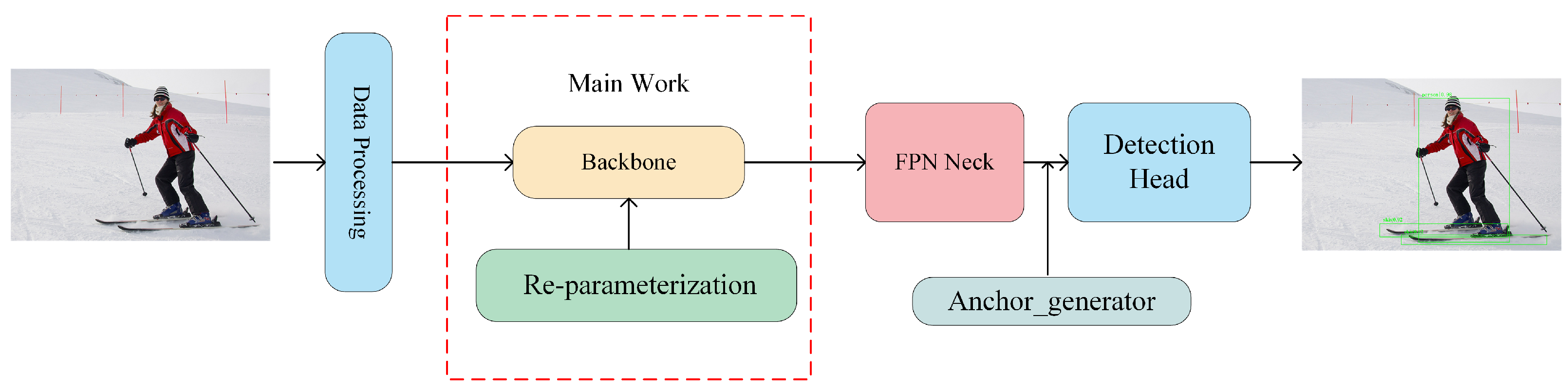
3.1. Design Ideas

Structural reparameterisation is a network compression technique that reduces the number of network parameters by clustering the convolutional kernels in a convolutional neural network and merging similar convolutional kernels into a new one. To demonstrate that the structural reparameterisation technique can improve the accuracy and speed of the object detection task, we propose a novel algorithmic framework for the object detection task, as shown in Figure 1.

The network model uses a structural reparameterisation-based backbone network, where the backbone network is a structural reparameterised VGG [27] network. Firstly, the images fed into the model are preprocessed, mainly by cropping and normalising them. Secondly, features are extracted from different stages of the backbone network, and the feature pyramid network is used to process multi-scale features and enhance the network’s ability to detect objects at different scales. The bottom–up FPN [8] network approach is used and the multi-scale feature maps are obtained by up-sampling and merging. In our network model, the FPN structure adopts the standard FPN structure and is fine-tuned in terms of the number of channels to better match the backbone network, with multiple-resolution feature map outputs. The network model then feeds the feature maps at all scales into the detection header, where a large number of prediction frames are generated on the feature maps at different scales to predict the class and location of the object. The output of the network results in a multi-scale detection result, for each of which the corresponding confidence scores and bounding box locations are calculated for filtering and merging. Finally, we used a novel NMS screening strategy in the screening phase to output the final detection results.

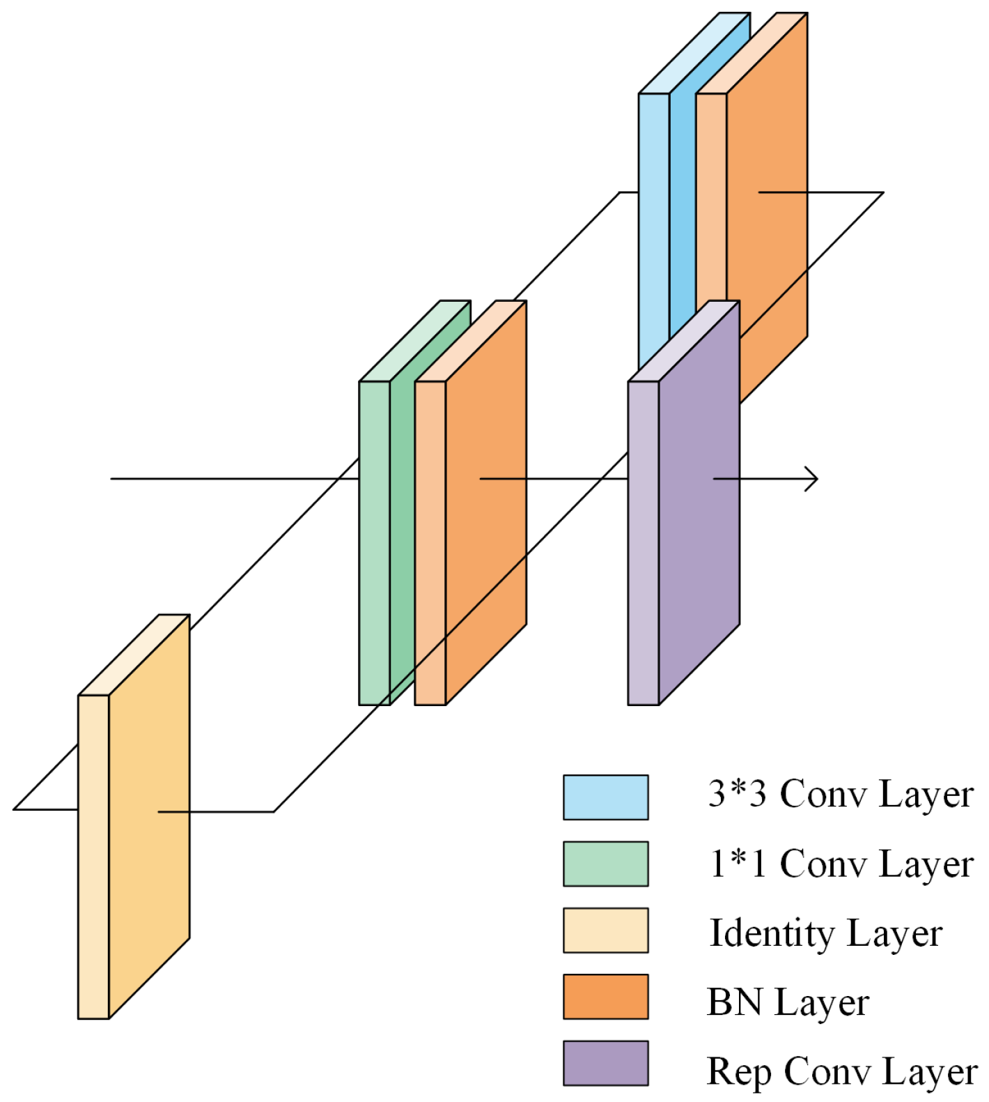
3.2. Structure Reparameterisation of the Backbone Network

The backbone network after structural reparameterisation is used as the backbone network of the whole model for extracting the basic image features. The reparameterised RepVGG [28] network has five stages, and each stage consists of a variable number of RepVGG blocks as [$n_1$, $n_2$, $n_3$, $n_4$, $n_5$], where $n_i$ denotes the number of RepVGG blocks in each stage. We designed two quantitative network models for detection, called the light-weight model RepRCNN-T and the medium-weight model RepRCNN-S. The number of RepVGG blocks in each stage of the light-weight model is set to [1, 2, 4, 14, 1], and the number of RepVGG blocks in each stage of the medium-weight model is set to [1, 4, 6, 16, 1] for each stage of the medium-weight model. In the reparameterisation phase, we merge the multi-branch structure into a single-branch structure, as shown in Figure 2. The multi-branch structure of the network is used in the training phase, and the merged single-branch structure is used in the inference phase. In the training phase, we use a three-branch structure for training the network, including the identity branch, 3 × 3 convolutional layers, and 1 × 1 convolutional layers, where BN layers are set after the convolutional layers for normalisation, but in the inference phase, we merge the three branches into one branch.

The fused convolutional layers are converted to Conv3×3, i.e., the convolution of specific different convolutional kernels are all converted to convolution with convolutional kernels of size 3 × 3. Since the whole residual block may contain both the Conv1×1 branch and identity branch, for the Conv1×1 branch, the whole conversion process is to replace the 1 × 1 convolution kernel with the 3 × 3 kernel, i.e., the value in the 1 × 1 kernel is moved to the centre of the 3 × 3 kernel, as shown in Figure 3. For the identity branch, this branch does not change the value of the input feature mapping, so we can set a 3 × 3 convolution kernel, and set the weight value at all 9 positions to 1. Then, it keeps the original value after multiplying with the input feature mapping. Merge the Conv3×3 in the residual branches and superimpose the weights W and bias B of all branches to obtain a fused Conv3×3 network layer after fusion.

For the merged convolutional layers, we fuse the convolutional and BN layers to perform accelerated computation operations in the training and inference phases. The strategy of fusing the convolutional and BN layers in a RepVGG block is mainly implemented by merging the convolutional and BN layers into a basic block. Each RepVGG block inside the module consists of two parts: one reparameterised convolutional layer and one nonlinear activation function, where the reparameterised convolutional layer consists of one 3 × 3 basic convolutional block and one BN layer, and after the nonlinear activation function in each block, we use the ReLU function. Specifically, as shown in Figure 4, each basic block consists of one normal convolutional layer, one BN layer, and one ReLU activation function, where the convolutional and BN layers are fused into a single learnable convolutional operation. During the training of the network, the gradient of the fused convolutional and BN parameters is simultaneously calculated and updated by the backpropagation algorithm of the network, thus enabling the end-to-end training of the network.

For the merging of 3 × 3 convolutional layers and BN layers, we generally ignored the bias b parameter in the convolutional layer of Equation (2) to achieve reparameterisation. Where W in Equation (2) denotes the parameters of the convolutional layer before conversion, the mean denotes the mean of the BN layer, Var denotes the variance of the BN layer, and gramma and beta denote the scale factor and offset factor of the BN layer, respectively. The convolution layer Equation (1) and BN layer Equation (2) in the residual block are fused by Equation (3). And, W′ and b′ in Equations (4) and (5) denote the weight and bias of the convolution after fusion, respectively.

$$Conv\left(x\right)=Wx+b$$

(1)

$$BN\left(x\right)=\gamma \ast \frac{x-Mean}{\sqrt{Var}}+\beta$$

(2)

$$BN(Com\left(x\right))=\frac{{\gamma }^{*}W}{\sqrt{Var}}\ast x+\beta -\frac{{\gamma }^{*}Mean}{\sqrt{Var}}$$

(3)

$$W^{\prime }=\frac{{\gamma }^{*}W}{\sqrt{Var}}$$

(4)

$$b^{\prime }=\frac{{\gamma }^{*}Mean}{\sqrt{Var}}-\beta$$

(5)

3.3. Attention Matching Strategies for Structural Branches

3.3.1. Characteristics of Different Branches

In traditional object detection networks, multiple branches are often used to extract different levels of feature information from the input image. These branches can capture low-level to high-level semantic information at different layers of the network, resulting in a multi-scale feature representation. In our approach, we use three branches to extract image information, called the 3 × 3 convolutional branch, the 1 × 1 convolutional branch, and the residual branch. These three branches focus on the global detail information, local feature information, and global context information of the image, respectively, and therefore can better acquire different levels and types of features.

When performing branch merging for structural reparameterisation, we consider that the three branches have their importance for image features. Among the three branches, the branch with 3 × 3 convolution has the global semantic information of the image features obtained in each stage, and the obtained features have a stronger representation ability on the whole; the branch with 1 × 1 convolution retains the main semantic information of the image features in the local context, which is helpful for us to obtain more accurate detection results; the residual branch mainly contains the original image feature information before convolution, which reflects the contextual semantic information. Based on the above reasons, if we simply weight the three branches to improve the speed, we will lose some valuable feature information, which will have an impact on the detection accuracy.

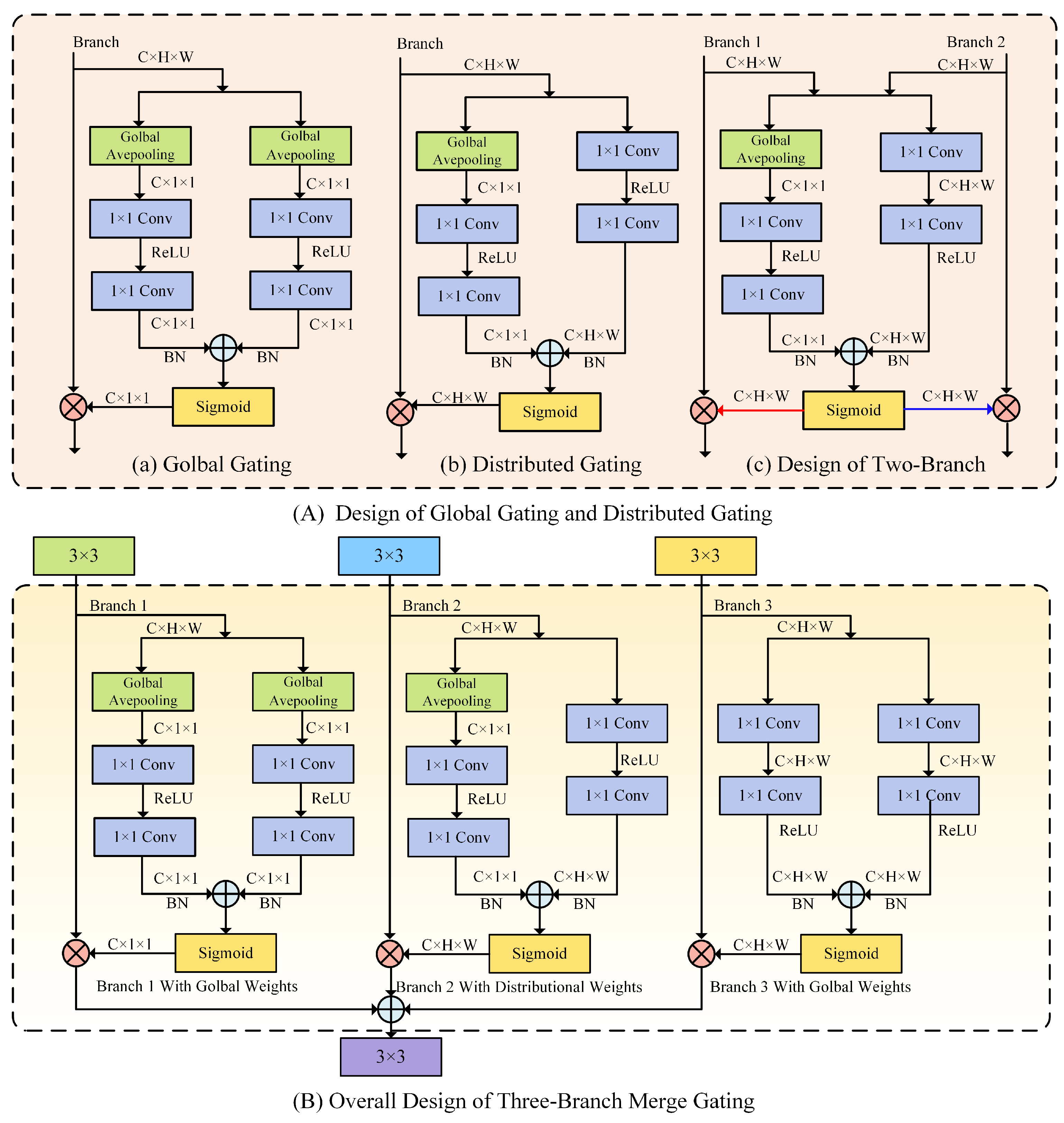
3.3.2. Three-Branch Merge Strategy

To improve the performance of the model, we explore two different branch merging strategies in the branch merging stage: direct branch merging and adaptive weight branch merging. The strategy of direct branch merging can save computational resources, but the default importance of all branches is equal, which cannot improve the effectiveness of important branches. The design of adaptive weight branch merging can effectively improve the weight of each branch and increase the importance of important branch weights to achieve the effect of improving accuracy. In order to illustrate the effects of the two strategies on the model, we design multiple sets of ablation experiments to analyse them in Section 4.4. According to the results of the ablation experiments in Section 4.4, after using adaptive weight branch merging, the adaptive weight branch merging strategy is more helpful to improve the detection performance compared to the base model.

3.3.3. Implementation of Control Branch-Matching Attention

In direct branch merging, we directly splice the features of the 3 × 3 convolutional branch, the 1 × 1 convolutional branch, and the residual branch, and merge them into a uniform-sized feature map, as shown in Figure 5A. However, this strategy, although simple, is prone to the problems of information redundancy and excessive dimensionality. In contrast, the adaptive weighted branch merging strategy allows us to introduce an “attention-like mechanism” to dynamically adjust the contribution of each branch. By introducing attention weights to determine the weight of each branch in the feature merging, the model can adaptively learn to efficiently combine the feature information from different branches, as shown in Figure 5B. This strategy avoids information redundancy while effectively exploiting the advantages of different branches, which improves the performance of the model.

To dynamically adjust the attention weights of each branch, we design different gating units to adjust and control the contributions of each branch concerning the characteristics of each branch. In Figure 6A, part(a) shows a single-branch global attention adaptive gating, part(b) shows a single-branch local attention adaptive gating, and part(c) shows a schematic of the application of two branches.

Specifically, we generate the attention weights using a lightweight gating unit that takes the branch features as input before fusion and undergoes convolution and global average pooling to obtain the attention weights. These weights are applied to the feature maps of each branch by matrix multiplication, enabling the adaptive weighting of different branch features. We apply this method to three branches, as shown in Figure 6B.

Firstly, the image features obtained in the 3 × 3 convolution branch in each stage have global semantic information, and we use global adaptive weighting on this branch. After the image features C × H × W are input into the global gating control after 3 × 3 convolution, in the two branches, they go through a global average pooling layer, a 1 × 1 convolutional layer, and a ReLU layer, respectively, to obtain the global adaptive weights with the size of C × 1 × 1, and after the sigmoid operation, the final result is obtained as a result of the size of C × 1 × 1 multiplied with the original input, to achieve the global adaptive control on the 3 × 3 convolutional branch.

Then, the 1 × 1 convolution branch locally retains the main semantic information of the image features, and we use local adaptive weighting on this branch. After the image feature C × H × W after 1 × 1 convolution is input into the local gating control, the global adaptive weights of size C × 1 × 1 are obtained in the first of the two branches by going through the global average pooling layer, 1 × 1 convolutional layer, and ReLU layer, and the local adaptive weights of size C × H × W are obtained in the second branch by going through the 1 × 1 convolutional layer and ReLU layer only. We sum up the results obtained from the two branches, and after the Sigmoid operation, the final result of size C × H × W is obtained by multiplying with the original input to achieve the local adaptive control of the 1 × 1 convolutional branch.

Finally, the residual branch mainly contains the original, pre-convolution image feature information, reflecting the contextual semantic information. We want to retain as much original contextual information as possible in this branch. After the image features C × H × W obtained from the residual branch are input into the third gating control, the same operation is performed in the two branches, which only passes through the 1 × 1 convolutional layer and the ReLU layer the adaptive weights with the size of C × H × W are obtained, and we believe that such an operation can retain contextual information in the residual branch. We sum the results obtained from the two results obtained from the branches are summed, and after the Sigmoid operation, the final result of size C × H × W is obtained by multiplying it with the original input to achieve the adaptive control of the residual branch.

We add the results of three gating and three branch multiplications as the final output, thus achieving attentional control over the three branches. Our strategy effectively learns the relationship between different branches and adjusts the contribution between the branches according to the needs of the task to achieve a better performance.

3.4. FPN Combined with Reparameterised Backbone Network

We divided the overall network into five stages after reparameterisation, and the image P1 input into the backbone network to extract features will gradually reduce the feature map size, and the final feature map used for detection tends to lose the detailed information of the large-scale feature maps due to the small scale. To be able to play a better role in general-purpose object detection, we add the FPN structure to the backbone network, which performs feature extraction on images of each scale and can produce multi-scale feature representations and feature maps of all levels with strong semantic information, even including some high-resolution feature maps. The structure of the backbone network combined with FPN is shown in Figure 7.

The fusion of the large-scale feature information P2, P3, P4, and the small-scale feature information P5 and P6 increases the low-level receptive field, enabling more contextual information to be obtained when performing the detection. Since the size of the feature map produced by each stage is adjustable, it is possible to combine the feature outputs from the FPN structure and each stage layer of the backbone network, and feed the fused feature map into the RPN [29] detection head for detection. Based on the feature pyramid, the RPN head is used to generate candidate frames for target classification and bounding box regression, and finally obtain the object detection results.

In the process of designing the algorithm, we also tried to reparameterise the FPN structure together with the backbone network to achieve a more concise structure and make the detection accelerate further. However, in practice, we only compared the model with the parameterised backbone network and the model with the parameterised backbone network and neck, and we found that the detection performance of the latter had a slight degradation, so the focus of our detection algorithm design is still on the backbone network.

3.5. Head Achieves Detection

In our network model, the FPN structure is used to extract feature maps at multiple scales from the input image, which have different scales and semantic information. These feature maps will be fed into head for object detection to produce detection results, as shown in Figure 8, which consists of two main parts, the RPN network and the classifier network.

In Figure 8, after receiving the feature map, the feature map is fed to the anchor generator to generate the feature map with the anchor box. Firstly, the generator generates H × W anchor points centred at each pixel on the H × W feature map. Then, anchor boxes are generated by applying different aspect ratios on the feature map for better target coverage. The sizes and ratios of these anchor frames are calculated from the datum frame, which has three main sizes, namely 512 × 512, 256 × 256, and 128 × 128. Nine anchor frames are generated on each anchor point according to the 1:1, 1:2, and 2:1 of the datum frame’s length and width.

The RPN section in Figure 8 performs classification and regression operations on the multiple anchor frames generated at each anchor point. Specifically, after generating the anchor box, the feature map is fed into the RPN part, which first performs one 3 × 3 convolutional layer to keep the feature map size, and then performs the computation of two 1 × 1 convolutional layers to achieve the binary classification task and the border regression task, respectively. For each anchor frame, it is determined whether the anchor frame is a target object (foreground) or background. Then, a regression operation is performed to adjust the position and size of the anchor frame to better match the real position of the target object. We generate proposals based on the results of classification and regression. We employ the NMS algorithm to filter the proposals. Each box containing the target is sorted from highest to lowest according to the classification score. After sorting each box, we calculate the IoU value for each box and for each box, when its value is above a certain threshold, it is removed from the box. Finally, the result is fed into the classifier. IoU is a commonly used value in detection tasks, and is the result of dividing the overlapping part of two regions by the aggregated part of the two regions, and comparing the result of this IoU calculation by a set threshold value. Generally, we consider that an object detection is recognised when the IoU is greater than the threshold value.

The classifier part in Figure 8 performs a second classification and regression operation on the filtered candidate boxes. The NMS screened candidate boxes are fed into RoIAlign, which corresponds to the feature map to obtain the corresponding features, providing input for subsequent tasks such as target classification and regression. The features on the grid of fixed-size feature maps generated by RoIAlign are fed into a classification network, which passes through the fully connected layer, and the classification score is used using a SoftMax activation function to convert to a probability distribution. Eventually, for each candidate box, a probability vector is obtained, indicating the probability that the candidate box belongs to different target categories. The regression operation is used to predict the bounding box offset values after going through the fully connected layer. These offset values are used to correct the position, width, and height of the candidate boxes to better match the true position of the target object.

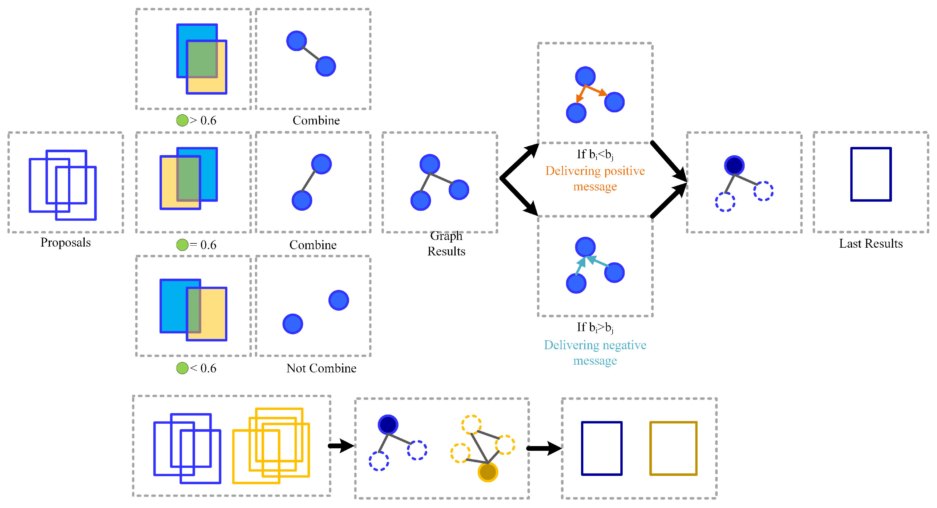
3.6. CPC NMS Strategy Application

A new graph-model-based bounding box clustering framework CP-Cluster is used in our detection model, which is fully parallelizable and can be used as a post-processing step of the object detector instead of the traditional soft-NMS method [30], called CPC NMS strategy [31]. Based on the CP-Cluster framework, we first convert all candidate frames into a collection of undirected graphs, where all frames with IoU less than a certain threshold belong to a graph. Then, in each graph, the nodes pass a positive message and negative message to each other simultaneously. Finally, while the duplicate boxes are eliminated, the confidence level of those selected boxes is enhanced. The strategy is shown in Figure 9.

For the CPC NMS strategy of Figure 9 [31], we first transform the multiple candidate boxes generated by the RPN into the form of a set of undirected graphs by defining each anchor box as a node and B = [$b_1$, $b_2$, $b_3$, …] is the original set of boxes output from the model before processing. For two boxes $b_i$, $b_j$ ($b_i$, $b_j$$\in B$), if their IoU is greater than the set threshold, we draw an undirected edge between them to generate a set of graphs G = [$g_1$, $g_2$, …]. In addition to the need to suppress redundant frames, it is also necessary to improve the confidence level of the real candidate frames. Specifically, we design positive messages $M_p$ to reward those true positive messages and negative messages $M_n$ [31], to penalise those redundant boxes. Both Mp and Mn only update the confidence values of the object boxes by default. As described in the previous section, positive messages are passed from the weaker object box to the stronger object box. Conversely, negative information flows from stronger object frames to weaker object frames. Candidate frames after filtering have higher confidence levels. Since each candidate box is affected by only one neighbour within a certain range, k threads can be created to process each box in parallel, where k is the number of candidate boxes.

3.7. Loss Function

For the loss function of the whole RepRCNN network, we combine the two losses in the RPN network therein, which consists of two parts, i.e., the category prediction loss and the target frame loss, and the two losses are linearly combined as shown in Equation (6):

$$L_{totall}\{(p_i,p_i^{*}),(b_i,{\widehat{b}}_{\widehat{\sigma }})\}=\sum _{i=1}^N[-\frac{1}{N}log[p{i}^{*}pi+(1-p{i}^{*})(1-pi)+{}_{\{c_i\ne ⌀\}}{\mathcal{L}}_{box}(b_i,{\widehat{b}}_{\widehat{\sigma }}\left(i\right))]$$

(6)

where y is the predicted value of the model, $\widehat{y}$ is the true value, and ${\mathbb{I}}_{\left\{c_i\ne ⌀\right\}}$ is a Boolean function that is 1 when $c_i\ne ⌀$. $c_i$ is the category label of the i object. ${\widehat{p}}_{\widehat{\sigma }\left(i\right)}\left(c_i\right)$ denotes the probability that the predicted $\sigma \left(i\right)$ prediction box has a category $c_i$. $b_i$ and ${\widehat{b}}_i$ are the true and predicted coordinates of the i object, respectively. ${\mathcal{L}}_{\mathrm{box}}$ is the distance between the two rectangular boxes.

For the classification task, we used cross entropy to calculate the loss between the result and the true target. $p_i$ denotes the probability that the output result is the target, and $p_i^{*}$ is a numerical value for the cross-concatenation ratio of the predicted result to the true value, which is greater than 0.5, $p_i^{*}$ = 1 and less than 0.5, $p_i^{*}$ = 0. We summed and averaged the entropy values to make a value of the loss for the classification task.

For the regression task, we use ${\mathcal{L}}_{\mathrm{box}}\left(·,·\right)$ for the calculation. Since the algorithm directly generates prediction frames for all scales, if the $l_1$ loss is used directly, the difference in the size of the loss value due to the different scales for small and large target frames makes the model more biased towards optimising the large-scale target frames. To alleviate this problem, a linear combination of $l_1$ loss and GIoU loss ${\mathcal{L}}_{\mathrm{iou}}\left(·,·\right)$ is used, which is scale-invariant, i.e., the effect on the loss function is the same regardless of whether it is for a large-scale prediction frame or a small-scale object frame. In total, the box loss is ${\mathcal{L}}_{\mathrm{box}}\left(b_i,{\widehat{b}}_{\widehat{\sigma }}\left(i\right)\right)$, as defined in Equation (7):

$${\mathcal{L}}_{\mathrm{box}}\left(b_i,{\widehat{b}}_{\widehat{\sigma }}\left(i\right)\right)={\lambda }_{\mathrm{iou}}{\mathcal{L}}_{\mathrm{iou}}\left(b_i,{\widehat{b}}_{\sigma \left(i\right)}\right)+{\lambda }_{\mathrm{L}1}{∥b_i-{\widehat{b}}_{\sigma \left(i\right)}∥}_1$$

(7)

where ${\lambda }_{\mathrm{iou}}$, ${\lambda }_{\mathrm{L}1}\in \mathrm{R}$, ${\mathcal{L}}_{\mathrm{iou}}\left(·,·\right)$ is the GIoU loss, as expressed as Equation (8):

$${\mathcal{L}}_{\mathrm{iou}}\left(b_{\sigma \left(i\right)},{\widehat{b}}_i\right)=1-\left(\frac{\left|b_{\sigma \left(i\right)}\bigcap {\widehat{b}}_i\right|}{\left|b_{\sigma \left(i\right)}\bigcup {\widehat{b}}_i\right|}-\frac{\left|B\left(b_{\sigma \left(i\right)},{\widehat{b}}_i\right)/b_{\sigma \left(i\right)}\bigcap {\widehat{b}}_i\right|}{\left|B\left(b_{\sigma \left(i\right)}{\widehat{b}}_i\right)\right|}\right)$$

(8)

3.8. Inference Process

We use a multi-branch structure to train our model, transforming the model into a single-branch structure in the inference phase. We take the network structure in the inference phase and build a structure similar to ResNet [32] by stacking multiple reparameterisation modules.

In the inference process, the test images are first preprocessed and then fed into the five stages of the parameterised backbone network to obtain the feature maps. A multi-scale feature pyramid is generated after the FPN network. Then, the feature map is input into RPN head, and after generating anchor points and anchor frames on the feature map, proposals are generated through the RPN section. Then, the improved NMS algorithm is used to filter the candidate frames that may contain the target. After the RoI align operation, the feature map region corresponding to each candidate box is divided into fixed-size sub-regions, and the features in the sub-regions are average-pooled to obtain the feature vector of each candidate box. These feature vectors are passed through the detection header and fed into multiple fully connected layers for predicting the class and location of the object. The final detection result includes the category, confidence, and location information for each detection frame.

4. Experiments

To verify the feasibility of the algorithm and the corresponding improvement effect, we conducted several experiments on the PASCAL VOC2012 dataset and MS COCO2017 dataset. The Nvidia RTX3090 GPU (NVIDIA Corporation, Santa Clara, CA, USA) environment was chosen, and all experiments were conducted under the system Ubuntu18.04 using the MMDetection framework. MMDetection is a PyTorch-based library of object detection tools, which currently contains dozens of models and methods.

4.1. Dataset

PASCAL VOC2012 is a classical computer vision dataset widely used for object detection, semantic segmentation, and image classification tasks. The dataset includes images from 20 different categories and contains a total of 17,125 images covering common object categories such as people, cars, planes, and animals.

MS COCO2017 is a large-scale dataset for tasks such as object detection, semantic segmentation, and image description. The dataset contains more than 330,000 images, including 328,000 training images and 41,000 validation images. These images are collected from a variety of scenarios, including scenes from daily life, natural landscapes, and industry. The MS COCO2017 dataset contains 80 common object categories, including people, animals, vehicles, electronic devices, furniture, and food. In addition, the dataset contains annotation information such as object bounding boxes, semantic segmentation masks, and instance segmentation masks associated with each image.

4.2. Baseline Criteria and Evaluation Metrics

Under the MMDetection framework, we chose the performance of two models, the classical faster R-CNN and cascade R-CNN, on the PASCAL VOC2012 and MS COCO2017 datasets as the baseline criteria. We also refer to the performance of current popular models such as DETR, DETR variants, and YOLO series on the two datasets. We also compare the experimental results with the OREPA model, which also employs the structural reparameterisation technique, and use this as a baseline for comparison as well.

The experimental evaluation metrics are mAP and AR, which are commonly used in object detection. mAP is an evaluation metric on the MS COCO2017 dataset commonly used to measure the accuracy of the object detection model, and the value of mAP ranges from 0 to 1, with a larger value indicating a more accurate detection result. AP50 and AP75 represent the detection accuracy at the IoU thresholds of 0.5 and 0.75, respectively. AR is the calculated detection recall for different categories of objects at all IoU thresholds, while the AR1000 metric represents the average detection recall for selecting the best 1000 candidate frames on each image to be evaluated at the time of testing.

4.3. Experimental Setup

We use RepRCNN-T and RepRCNN-S as representatives of the lightweight and mediumweight models, respectively. We vary the number of reparameterisation modules in each stage and set them to [1, 2, 4, 14, 1] and [1, 4, 6, 16, 1], respectively, with the lightweight model being suitable for tasks that require a high detection speed and the middleweight model being suitable for tasks that require a high detection accuracy.

Following the official PyTorch example, we use a global batch of size 8, initialised to a learning rate of 0.001, with a weight recession set to 1.0 $\times {10}^{-4}$ and a standard SGD optimiser (momentum factor of 0.9) on a single GPU. The model was trained using a cross-entropy loss function and a regression loss function. The maximum basic clipping size of the dataset was kept as (1333, 800), an image inversion probability of 0.5 was used for both, the same image normalisation operation as in the baseline, and the minimum unit for Resize of the image was set to 32. We used 32-bit floating point numbers (single precision) on our device, the NVIDIA 3090, to represent the weights and activation values of the network, which provided sufficient numerical precision to handle the object detection task and maintain model performance.

Different ablation experiments were also designed by continuously adjusting the hyperparameters during the experiment to achieve optimal experimental results. The model performance metrics are evaluated separately in the experimental part in a cycle of 24 rounds. To illustrate the enhancement of network performance by branch-matching reparameterisation, a before-and-after comparison of the model testing results is performed.

4.4. Ablation Experiments

We first investigated the changes in performance before and after the model of the reparameterisation approach and made adjustments accordingly based on the results. The effectiveness of the combination of the reparameterisation strategy and the new NMS strategy on the model is demonstrated by improving the lightweight Base model. For the CPC NMS strategy, since CPC does not require retraining the model, we download popular models from MMDetection and evaluated them by CPC. The results of the ablation experiments on the MS COCO2017 dataset are reported in

Table 1. Ablation experimental performance.

Method	NMS	CPC	Rep	mAP	Parameter	Inf Time	Round
Base	N	N	N	37.6	45 M	12.1	1×
Base+NMS	Y	N	N	37.7	45 M	11.9	1×
Base+CPC	N	Y	N	38.1	45 M	12.5	1×
Base+Rep	N	N	Y	38.7	38 M	13.9	1×
Base+Rep+NMS	Y	N	Y	39.1	38 M	14.2	1×
Base+Rep+CPC	N	Y	Y	39.5	38 M	14.1	1×

The meaning of Y in the table is that the method of the column was used, i.e., yes. The meaning of N in the table is that the method of the column was not used, i.e., no. The meaning of 1× is after one training cycle and each training cycle is 12 epochs.

and Figure 10.

As can be seen from Table 1 and Figure 9, after using CPC NMS, the mAP of the model is improved compared to standard NMS. Compared with the standard NMS, after using CPC, it can improve the mAP while maintaining a certain FPS, which proves that our method is effective. Meanwhile, from the presentation of experimental data about reparameterisation, we can conclude that the network model with reparameterisation has reduced in terms of the number of parameters during the training period, which meets our expected criteria. In terms of mAP metrics and FPS metrics, it can be seen that the new model maintains better results. In particular, the model performance is significantly improved by the use of the reparameterisation approach and the CPS NMS strategy.

For the branch-matching reparameterisation strategy,

Table 2. Experimental performance of branch-matched ablation.

Method	3 × 3 Branch	1 × 1 Branch	Residual	mAP
Base	None	None	None	51.7
Base+ Branch Matching	Global	Global	Global	53.0
	Global	Distributions	Global	53.2
	Distributions	Global	Global	52.2
	Distributions	Distributions	Global	51.5

shows the performance change of our model on the PASCAL VOC2012 dataset before and after using the branch-matching strategy, and we actively explored the use of different gating for the three branches.

As can be seen in Table 2, the mAP of the model changes after using the adaptive weight branch-merging strategy. Compared to the base model without branch matching, the model performance improves when the appropriate gating type is selected on all three branches. When using global gating units on all three branches, the mAP improves by 1.3. The greatest performance improvement is achieved when using global gating on the 3 × 3 branch and the residual branch, and local gating only on the 1 × 1 branch, with an increase in mAP of 1.5. The performance of the model decreases when we try to use local gating on a larger number of branches. Based on the ablation experiments described above, we chose to apply global gating on the 3 × 3 branch, local gating on the 1 × 1 branch, and global gating on the residual branch.

4.5. Experimental Results and Analyses

4.5.1. PASCAL VOC2012 Performance

In pursuit of better the accuracy performance in the detection process, we discard the training speed to see the extreme performance of each baseline model and our model in terms of accuracy on the PASCAL VOC2012 dataset. The training period is set to 24 epochs to explore the best performance of the model in terms of detection accuracy. Eventually, the location where our model converges is explored and compared with the baseline model, and the experimental results are shown in

Table 3. Model performance on PASCAL VOC2012.

Method	Backbone	Train Data	mAP	AP50	AP75
Faster RCNN [5]	VGG-16	VOC2012	–	67	–
		VOC2007+2012	–	70.4	–
		COCO+VOC2007+2012	–	75.9	–
Ca.RCNN [6]	AlexNet	VOC2007	38.9	66.5	40.5
	VGG-16		51.2	79.1	56.3
	ResNet-50		51.8	78.5	57.1
KL loss [24]	ResNet-50	VOC2007	–	75.8	–
Co-teaching [33]	ResNet-50	VOC2007	–	75.4	–
SD-LocNet [34]	ResNet-50	VOC2007	–	75.7	–
FreeAnchor [35]	ResNet-50	VOC2007	–	73.0	–
OA-MIL [13]	ResNet-50	VOC2007	–	77.4	–
SSD-Det [36]	ResNet-50	VOC2007	–	77.1	–
DETR/150 [11]	ResNet-50	VOC2007	49.9	74.5	53.4
DETR/300 [11]	ResNet-50	VOC2007	54.1	78.0	58.3
YOLOX-T [37]	ResNet-50	VOC2012	35.4	57.9	–
YOLOX-S [37]	ResNet-50	VOC2012	42.6	64.5	–
RepModel	RepRCNN-S	VOC2012	51.6	75.8	56.2
	RepRCNN-S	COCO+VOC2012	53.2	78.4	58.1

.

With the experimental data in Table 3, we can see that the models using the branch-and-merge reparameterisation models all have performance gains compared to the baseline model. After training 24 epochs on PASCAL VOC2012 using RepRCNN-S, we achieved accuracies of 51.6, 75.8, and 56.2 for mAP, AP50, and AP75, respectively, which further confirms the effectiveness of the branch-merging strategy.

To further improve the performance of the model on the PASCAL VOC2012 dataset, we adopt a training strategy similar to that of faster RCNN, We first expand the training set of the model to the training concatenation of MS COCO2017 and PASCAL VOC2012, and then use the model to test it on PASCAL VOC2012, and the experimental results are similar to that of only training on PASCAL VOC2012. The experimental results are competitive with mainstream models. RepRCNN-S outperforms faster R-CNN with the same training method by 2.5. RepRCNN-S and DETCNN with only 150 epochs are more competitive than DETCNN with only 150 epochs. RepRCNN-S has 3.3, 3.9, and 4.7 higher mAP, AP50, and AP75, respectively, compared with DETR trained with only 150 epochs. We note, however, that the accuracy of DETR after 300 epochs is also substantially improved, but DETR is much more computationally intensive than our model, so from the computational cost point of view, RepModel has a better speed–accuracy balance.

4.5.2. MS COCO2017 Performance

We similarly view the limiting performance of each baseline model and our model in terms of accuracy on the MS COCO2017 dataset.

Table 4. Model performance on MS COCO2017.

Method	Backbone	mAP	AP50	AP75	Parameters	Inf Time
KL loss [24]	ResNet-50	31.0	54.3	30.3	–	–
Co-teaching [33]	ResNet-50	30.5	54.9	30.5	–	–
SD-LocNet [34]	ResNet-50	30.0	54.5	30.3	–	–
FreeAnchor [35]	ResNet-50	28.6	53.1	28.5	–	–
OA-MIL [13]	ResNet-50	32.1	55.3	33.2	–	–
OREPA [22]	ResNet-50	37.4	–	–	–	–
DETR [11]	ResNet-50	42.0	62.4	44.2	–	–
UP-DETR [12]	ResNet-50	42.8	63.0	45.3	–	–
YOLOV3 [3]	Darknet-53	36.2	60.6	38.2	–	–
Faster RCNN [5]	ResNet-50	37.7	59.2	40.9	25 M	13.6
	ResNet-101	40.0	61.8	43.7	45 M	11.9
Ca.RCNN [6]	ResNet-50	41.3	59.4	45.3	25 M	11.9
	ResNet-101	43.3	61.7	47.2	45 M	10.3
YOLOX-T [37]	PANet	32.8	50.3	–	5.1 M	7.1
YOLOX-S [37]	PANet	40.5	59.3	–	9 M	15.0
YOLOv6-T [4]	EfficientRep	40.3	56.6	–	15 M	11.1
YOLOv6-S [4]	EfficientRep	43.2	60.4	–	17.2 M	12.9
YOLOv7-T [1]	EfficientRep	37.4	55.2	–	6.2 M	11.8
RepModel	RepRCNN-T	41.2	59.7	43.5	14 M	14.1
	RepRCNN-S	42.0	61.4	44.1	38 M	12.3
New RepModel	RepRCNN-T	41.8	60.2	43.7	14 M	14.1
	RepRCNN-S	43.3	62.1	45.6	38 M	12.3

and

Table 5. AR1000 performance of the model on 24 epochs training.

Model	Backbone	AR1000	Parameter	Training Time	Inf Time	Round
RPN	Resnet-50	57.6	25M	–	17.7	2×
	Resnet-101	59.1	45M	–	14.4	2×
RepRCNN	RepRCNN-T	58.6	14M	0.449	18.2	2×
	RepRCNN-S	59.9	38M	0.512	15.6	2×

The meaning of 2× is after one training cycle and each training cycle is 24 epochs.

show the mAP and AR1000 performances of the models on the MS COCO2017 dataset, respectively.

From the experimental data in Table 4, we can see that, except for the training time and inference speed, the parameterised models have improved performance compared to the baseline model. RepRCNN-T and RepRCNN-S still maintained an advantage in FPS metrics, which are 14.1 FPS and 12.3 FPS, respectively. Compared with the similar reparameterised models, OREPA RepRCNN-T and RepRCNN-S both have excellent performances. In terms of detection accuracy, we achieved 41.8, 60.2, and 43.7 for mAP, AP50, and AP75, respectively, after 24 epochs of training on the MS COCO2017 dataset using RepRCNN-T, and 43.3, 62.1, and 45.6 for mAP, AP50, and AP75, respectively, using RepRCNN-S. After using branch matching before and after use, the model performance improves at mAP, AP50, and AP75 by 1.3, 0.7, and 1.5, respectively.

With a similar number of parameters, the model with a branch-matching strategy is more competitive compared to the lightweight networks of YOLOv6 and YOLOv7. RepRCNN-T improves mAP, AP50 by 1.5, 3.6 compared to YOLOv6-T; RepRCNN-S improves mAP, AP50 by 0.1 compared to YOLOv6-S, 1.7; mAP improves by 1.3 compared to the mainstream model DETR, and mAP improves by 0.5 compared to the variant UP-DETR. In terms of detection speed, our model ranks second with an FPS of 14.1 but has a higher detection accuracy than the fastest YOLOX-S, considering that the computational overheads and training time of DETR and the variant UP-DETR are much higher than the RepModel, which maintains a better accuracy and achieves a better speed–accuracy balance.

With the data in Table 5, we can see that, with the gradual deepening of the network and the increase in the number of training rounds, our model significantly improved the metrics in AR1000 compared to the RPN network, and in terms of accuracy performance, RepRCNN-T and RepRCNN-S are higher by 1 and 0.8, respectively.

Different IoU thresholds were also used to compute the P–R curves in our object detection task, as shown in Figure 11.

From Figure 11, we can see that, at high thresholds, our model has higher accuracy, while at low thresholds, our model has higher recall. This indicates that our model can capture more targets when detecting them. Therefore, our model has better performance and adaptability.

4.5.3. Visualisation of Detection Results

We visualised the detection results for the MS COCO2017 dataset. The four photos in Figure 12 show the results when the scene is more homogeneous and has less object detection, and the four photos in Figure 13 show the results when the scene is complex and has more object detection.

From the demonstrated results in Figure 12, in the case of a simpler scene situation with fewer targets, and with sufficient light and unobstructed targets, our model can detect the objects contained in the picture to be detected and gives a high level of confidence that the detection results are very accurate.

From the demonstration effect in Figure 13, in the case of a more complex scene with a larger number of objects to be detected and the presence of occlusion between multiple objects, our model is still able to maintain the detection of the main objects in the picture to be detected and give a reasonable confidence level. For most of the occluded targets, the model is also able to detect and classify the corresponding objects, showing a good detection performance.

5. Conclusions

With the rapid development of deep learning technology applications in the field of computer vision, deep learning-based object detection algorithms have become mainstream methods. However, the application of deep learning in the field of object detection also faces some challenges, such as how to better balance detection accuracy and speed, algorithm interpretability, and computational resource limitations. Aiming to resolve the problem of balancing accuracy and speed in object detection techniques, a CNN object detection method based on a structural reparameterisation technique using branch matching is proposed. We use a neural network after structural reparameterisation with branch matching for the detection task, by which the technique reduces the number of parameters in the network and saves the storage overhead and computational overhead in the inference process. For real-time detection, the structural reparameterisation technique can significantly improve the detection speed of the model, which is advantageous in terms of FPS. Structural reparameterisation techniques have good performance in detection tasks that require speed aspects but lose some accuracy. As a result, reparameterisation techniques tend to be less suitable for applications in tasks that require higher accuracy.

References

1. Wang, C.Y.; Bochkovskiy, A.; Liao, H.Y.M. YOLOv7: Trainable bag-of-freebies sets new state-of-the-art for real-time object detectors. In Proceedings of the IEEE/CVF Conference on Computer Vision and Pattern Recognition, Vancouver, BC, Canada, 18–22 June 2023; pp. 7464–7475. [Google Scholar]
2. Liu, W.; Anguelov, D.; Erhan, D.; Szegedy, C.; Reed, S.; Fu, C.Y.; Berg, A.C. Ssd: Single shot multibox detector. In Proceedings of the Computer Vision–ECCV 2016: 14th European Conference, Amsterdam, The Netherlands, 11–14 October 2016; Proceedings Part I 14. Springer: Berlin, Germany, 2016; pp. 21–37. [Google Scholar]
3. Redmon, J.; Farhadi, A. Yolov3: An incremental improvement. arXiv 2018, arXiv:1804.02767. [Google Scholar]
4. Li, C.; Li, L.; Jiang, H.; Weng, K.; Geng, Y.; Li, L.; Ke, Z.; Li, Q.; Cheng, M.; Nie, W.; et al. YOLOv6: A single-stage object detection framework for industrial applications. arXiv 2022, arXiv:2209.02976. [Google Scholar]
5. Ren, S.; He, K.; Girshick, R.; Sun, J. Faster r-cnn: Towards real-time object detection with region proposal networks. arXiv 2015, arXiv:1506.01497. [Google Scholar] [CrossRef] [PubMed]
6. Cai, Z.; Vasconcelos, N. Cascade r-cnn: Delving into high quality object detection. In Proceedings of the IEEE Conference on Computer Vision and Pattern Recognition, Salt Lake City, UT, USA, 18–22 June 2018; pp. 6154–6162. [Google Scholar]
7. Cai, Z.; Fan, Q.; Feris, R.S.; Vasconcelos, N. A unified multi-scale deep convolutional neural network for fast object detection. In Proceedings of the Computer Vision–ECCV 2016: 14th European Conference, Amsterdam, The Netherlands, 11–14 October 2016; Proceedings, Part IV 14. Springer: Berlin, Germany, 2016; pp. 354–370. [Google Scholar]
8. Lin, T.Y.; Dollár, P.; Girshick, R.; He, K.; Hariharan, B.; Belongie, S. Feature pyramid networks for object detection. In Proceedings of the IEEE Conference on Computer Vision and Pattern Recognition, Honolulu, HI, USA, 21–26 July 2017; pp. 2117–2125. [Google Scholar]
9. Lin, T.Y.; Goyal, P.; Girshick, R.; He, K.; Dollár, P. Focal loss for dense object detection. In Proceedings of the IEEE International Conference on Computer Vision, Venice, Italy, 22–29 October 2017; pp. 2980–2988. [Google Scholar]
10. Woo, S.; Park, J.; Lee, J.Y.; Kweon, I.S. Cbam: Convolutional block attention module. In Proceedings of the European Conference on Computer Vision (ECCV), Munich, Germany, 8–14 September 2018; pp. 3–19. [Google Scholar]
11. Carion, N.; Massa, F.; Synnaeve, G.; Usunier, N.; Kirillov, A.; Zagoruyko, S. End-to-end object detection with transformers. In Proceedings of the European Conference on Computer Vision, Glasgow, UK, 23–28 August 2020; pp. 213–229. [Google Scholar]
12. Dai, Z.; Cai, B.; Lin, Y.; Chen, J. Up-detr: Unsupervised pre-training for object detection with transformers. In Proceedings of the IEEE/CVF Conference on Computer Vision and Pattern Recognition, Nashville, TN, USA, 20–25 June 2021; pp. 1601–1610. [Google Scholar]
13. Liu, C.; Wang, K.; Lu, H.; Cao, Z.; Zhang, Z. Robust Object Detection with Inaccurate Bounding Boxes. In Proceedings of the European Conference on Computer Vision, Tel Aviv, Israel, 23–27 October 2022; pp. 53–69. [Google Scholar]
14. Han, S.; Mao, H.; Dally, W.J. Deep compression: Compressing deep neural networks with pruning, trained quantization and huffman coding. arXiv 2015, arXiv:1510.00149. [Google Scholar]
15. Malsagov, M.Y.; Khayrov, E.M.; Pushkareva, M.M.; Karandashev, I.M. Exponential discretization of weights of neural network connections in pre-trained neural networks. Opt. Mem. Neural Netw. 2019, 28, 262–270. [Google Scholar] [CrossRef]
16. Hinton, G.; Vinyals, O.; Dean, J. Distilling the knowledge in a neural network. arXiv 2015, arXiv:1503.02531. [Google Scholar]
17. Redmon, J.; Farhadi, A. YOLO9000: Better, faster, stronger. In Proceedings of the IEEE Conference on Computer Vision and Pattern Recognition, Honolulu, HI, USA, 21–26 July 2017; pp. 7263–7271. [Google Scholar]
18. Ding, X.; Zhang, X.; Han, J.; Ding, G. Scaling up your kernels to 31x31: Revisiting large kernel design in cnns. In Proceedings of the IEEE/CVF Conference on Computer Vision and Pattern Recognition, New Orleans, LA, USA, 18–24 June 2022; pp. 11963–11975. [Google Scholar]
19. Liu, Z.; Lin, Y.; Cao, Y.; Hu, H.; Wei, Y.; Zhang, Z.; Lin, S.; Guo, B. Swin transformer: Hierarchical vision transformer using shifted windows. In Proceedings of the IEEE/CVF International Conference on Computer Vision, Montreal, BC, Canada, 11–17 October 2021; pp. 10012–10022. [Google Scholar]
20. Ding, X.; Xia, C.; Zhang, X.; Chu, X.; Han, J.; Ding, G. Repmlp: Re-parameterizing convolutions into fully-connected layers for image recognition. arXiv 2021, arXiv:2105.01883. [Google Scholar]
21. Ding, X.; Zhang, X.; Han, J.; Ding, G. Diverse branch block: Building a convolution as an inception-like unit. In Proceedings of the IEEE/CVF Conference on Computer Vision and Pattern Recognition, Nashville, TN, USA, 20–25 June 2021; pp. 10886–10895. [Google Scholar]
22. Hu, M.; Feng, J.; Hua, J.; Lai, B.; Huang, J.; Gong, X.; Hua, X.S. Online convolutional re-parameterization. In Proceedings of the IEEE/CVF Conference on Computer Vision and Pattern Recognition, New Orleans, LA, USA, 18–24 June 2022; pp. 568–577. [Google Scholar]
23. Chu, X.; Li, L.; Zhang, B. Make RepVGG Greater Again: A Quantization-aware Approach. arXiv 2022, arXiv:2212.01593. [Google Scholar]
24. He, Y.; Zhu, C.; Wang, J.; Savvides, M.; Zhang, X. Bounding box regression with uncertainty for accurate object detection. In Proceedings of the IEEE/CVF Conference on Computer Vision and Pattern Recognition, Long Beach, CA, USA, 15–20 June 2019; pp. 2888–2897. [Google Scholar]
25. Ning, C.; Zhou, H.; Song, Y.; Tang, J. Inception single shot multibox detector for object detection. In Proceedings of the 2017 IEEE International Conference on Multimedia & Expo Workshops (ICMEW), Hong Kong, China, 10–14 July 2017; pp. 549–554. [Google Scholar]
26. He, Y.; Zhang, X.; Savvides, M.; Kitani, K. Softer-nms: Rethinking bounding box regression for accurate object detection. arXiv 2018, arXiv:1809.08545. [Google Scholar]
27. Simonyan, K.; Zisserman, A. Very deep convolutional networks for large-scale image recognition. arXiv 2014, arXiv:1409.1556. [Google Scholar]
28. Ding, X.; Zhang, X.; Ma, N.; Han, J.; Ding, G.; Sun, J. Repvgg: Making vgg-style convnets great again. In Proceedings of the IEEE/CVF Conference on Computer Vision and Pattern Recognition, Nashville, TN, USA, 20–25 June 2021; pp. 13733–13742. [Google Scholar]
29. Brazil, G.; Liu, X. M3d-rpn: Monocular 3d region proposal network for object detection. In Proceedings of the IEEE/CVF International Conference on Computer Vision, Seoul, Republic of Korea, 27 October–2 November 2019; pp. 9287–9296. [Google Scholar]
30. Bodla, N.; Singh, B.; Chellappa, R.; Davis, L.S. Soft-NMS–improving object detection with one line of code. In Proceedings of the IEEE International Conference on Computer Vision, Venice, Italy, 22–29 October 2017; pp. 5561–5569. [Google Scholar]
31. Shen, Y.; Jiang, W.; Xu, Z.; Li, R.; Kwon, J.; Li, S. Confidence propagation cluster: Unleash full potential of object detectors. In Proceedings of the IEEE/CVF Conference on Computer Vision and Pattern Recognition, New Orleans, LA, USA, 18–24 June 2022; pp. 1151–1161. [Google Scholar]
32. He, K.; Zhang, X.; Ren, S.; Sun, J. Deep residual learning for image recognition. In Proceedings of the IEEE Conference on Computer Vision and Pattern Recognition, Las Vegas, NV, USA, 26 June–1 July 2016; pp. 770–778. [Google Scholar]
33. Han, B.; Yao, Q.; Yu, X.; Niu, G.; Xu, M.; Hu, W.; Tsang, I.; Sugiyama, M. Co-teaching: Robust training of deep neural networks with extremely noisy labels. arXiv 2018, arXiv:1804.06872. [Google Scholar]
34. Zhang, X.; Yang, Y.; Feng, J. Learning to localize objects with noisy labeled instances. In Proceedings of the AAAI Conference on Artificial Intelligence, Honolulu, HI, USA, 27 January–1 February 2019; Volume 33, pp. 9219–9226. [Google Scholar]
35. Zhang, X.; Wan, F.; Liu, C.; Ji, R.; Ye, Q. Freeanchor: Learning to match anchors for visual object detection. arXiv 2019, arXiv:1909.02466. [Google Scholar]
36. Wu, D.; Chen, P.; Yu, X.; Li, G.; Han, Z.; Jiao, J. Spatial Self-Distillation for Object Detection with Inaccurate Bounding Boxes. arXiv 2023, arXiv:2307.12101. [Google Scholar]
37. Zhou, W.; Min, X.; Hu, R.; Long, Y.; Luo, H. FasterX: Real-Time Object Detection Based on Edge GPUs for UAV Applications. arXiv 2022, arXiv:2209.03157. [Google Scholar]
Figure 1. Schematic diagram of the algorithm framework.
Electronics 12 04180 g001
Figure 2. Schematic diagram of merging three branches into a single branch.
Electronics 12 04180 g002
Figure 3. Illustration of heavy parameter merging.
Electronics 12 04180 g003
Figure 4. Schematic diagram of the merged structure.
Electronics 12 04180 g004
Figure 5. Schematic diagram of branch-matching merge.
Electronics 12 04180 g005
Figure 6. Detailed structural diagram of the three-branch-matching design.
Electronics 12 04180 g006
Figure 7. Combination schematic.
Electronics 12 04180 g007
Figure 8. Head structure diagram.
Electronics 12 04180 g008
Figure 9. CPC NMS strategy diagram.
Electronics 12 04180 g009
Figure 10. Histogram of ablation experiment results.
Electronics 12 04180 g010
Figure 11. P–R curves at different thresholds.
Electronics 12 04180 g011
Figure 12. The effect of simple scene detection.
Electronics 12 04180 g012
Figure 13. The effect of complex scene detection.
Electronics 12 04180 g013