Article

Global Individual Interaction Network Based on Consistency for Group Activity Recognition

1
School of Electronics and Information Technology, Sun Yat-sen University, Guangzhou 510006, China
2
Department of Electrical and Computer Engineering, Brigham Young University, Provo, UT 84602, USA
*
Author to whom correspondence should be addressed.
Electronics 2023, 12(19), 4104; https://doi.org/10.3390/electronics12194104
Submission received: 12 September 2023 / Revised: 29 September 2023 / Accepted: 29 September 2023 / Published: 30 September 2023
(This article belongs to the Special Issue Advances of Artificial Intelligence and Vision Applications)

Abstract

:
Modeling the interactions among individuals in a group is essential for group activity recognition (GAR). Various graph neural networks (GNNs) are regarded as popular modeling methods for GAR, as they can characterize the interaction among individuals at a low computational cost. The performance of the current GNN-based modeling methods is affected by two factors. Firstly, their local receptive field in the mapping layer limits their ability to characterize the global interactions among individuals in spatial–temporal dimensions. Secondly, GNN-based GAR methods do not have an efficient mechanism to use global activity consistency and individual action consistency. In this paper, we argue that the global interactions among individuals, as well as the constraints of global activity and individual action consistencies, are critical to group activity recognition. We propose new convolutional operations to capture the interactions among individuals from a global perspective. We use contrastive learning to maximize the global activity consistency and individual action consistency for more efficient recognition. Comprehensive experiments show that our method achieved better GAR performance than the state-of-the-art methods on two popular GAR benchmark datasets.

1. Introduction

Group activity recognition (GAR) classifies the collective behavior of a group of people in a short video clip of a specific event based on the individual actions of the group members and their interactions with each other [1]. Different from deep learning tasks, such as human activity recognition [2], people tracking [3], and occupancy counting [4], GAR is unique in its potential to explore critical semantic information from interactions among individuals and thus widely used in security surveillance, social role understanding, and sports video analysis.
A big challenge for GAR is to characterize the distinctive property of interactions among individuals in a group. Almost all early GAR methods [5,6,7] used hand-crafted features to describe the interactions among individuals. The performance of these methods was limited due to their inability to extract semantic features from the video frames. Machine learning-based, especially deep learning, methods are capable of learning features at various levels of abstraction from the training data to obtain better performance than those using hand-crafted features. Among the recent deep learning methods, multi-head self-attention networks (MHSA)-based methods [8,9,10] achieved the best performance with a global receptive field, although not being computationally efficient. Graphs have shown great success in characterizing the structure of a group and the interactions existing in a group in recent years. Some state-of-the-art deep learning-based GAR methods used graphs to learn meaningful features through innovations in interaction modeling and achieved promising results.
To characterize the interactions among individuals in the group, many state-of-the-art deep learning-based GAR methods learn the features of interactions of each person with others in the neighborhood in each frame and characterize the interactions among them with graphs. Early graph neural networks (GNNs)-based methods [11,12] are well suited to model these interactions, but their predefined connectivity is not flexible for every individual’s interactions with others [13]. The dynamic inference network (DIN) [13] takes advantage of the deformable convolutional network (DCN) [14] to generate dynamic convolutional sampling positions and provide a description of group activity that can suit every individual’s interactions with others in the group. A significant challenge for the existing GAR methods is that their models only consider the interactions of each person with their neighbors to characterize their influence on group activity. They do not consider the influence from other individuals.
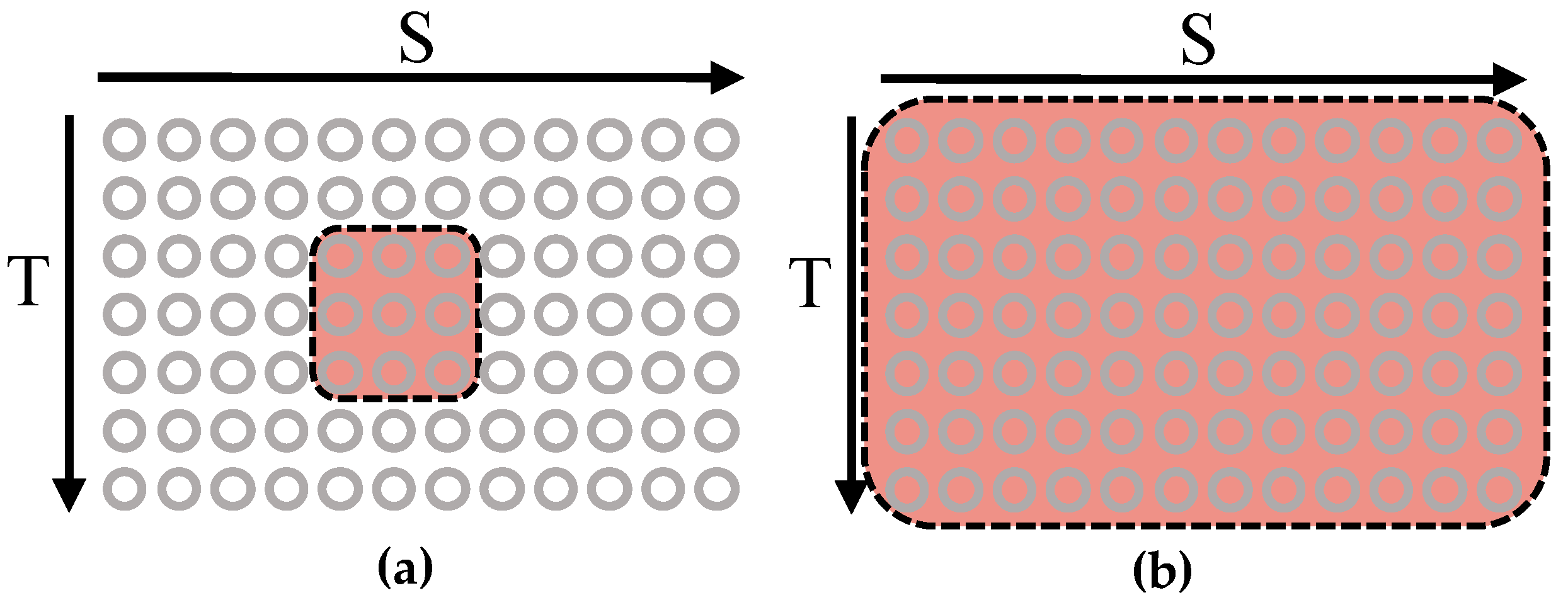
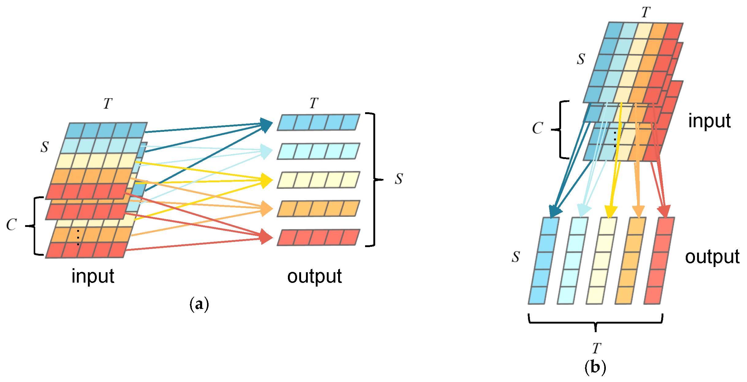
Current GNN-based methods usually use mapping layers [11,12,13], i.e., normal convolutional layers with a receptive field of 3 × 3 as shown in Figure 1a, or fully connected layers with a receptive field of 1 × 1 in both spatial and temporal dimensions to describe the interactions of each individual with their neighbors. Each circle in Figure 1 represents the feature of the state of an individual action in one frame. The horizontal (S) axis represents the indexes of individuals in the group according to their locations in the x-axis of the image. The vertical (T) axis represents the indexes of the image frames in the group action video clip. The red-shaded area represents the local receptive field centered around an individual for the mapping layer used in the existing methods [11,12,13]. Although these approaches [11,12,13] simplify the computation and reduce the computation cost, they fail to catch the features of global interaction patterns or the influence from all other individuals involved in the group activity.
To obtain better GAR performance, the distinctive pattern of group activity should consider the global interactions among individuals, i.e., the interactions among all group members throughout the video of the entire event. Learning the interaction pattern of a group activity from a global viewpoint is critical to improving GAR performance. Using mapping layers with a global receptive field in the spatial–temporal dimensions helps the network to capture the interactions among all individuals [8,9,10]. The mapping layer with the global receptive field (shown in Figure 1b) involves the locations of all members in the group and all image frames in the event video when computing, and it is computationally expensive. Characterizing global interactions involved in group activity efficiently remains an open challenge.
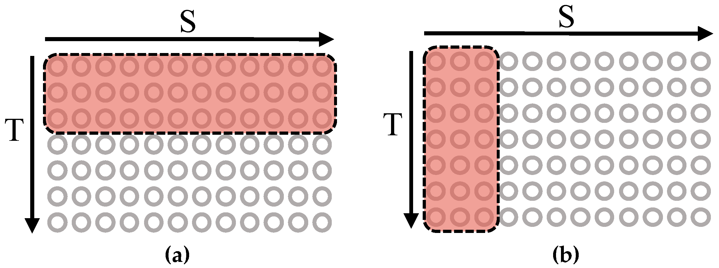
In this paper, we propose a new GNN-based network to recognize group activity in videos. This new network contains two new convolution layers that focus on characterizing the global interactions of group activity efficiently while maintaining reasonable computational requirements. One convolution layer, as shown in Figure 2a, is designed with a global receptive field in the spatial dimension (S) and a local receptive field in the temporal dimension (T). The second convolutional layer, as shown in Figure 2b, has a local receptive field in the spatial dimension (S) and a global receptive field in the temporal dimension (T). These two designed convolutional layers allow our new network to use two kinds of global receptive fields in the spatial and temporal dimensions separately to provide an improved ability to capture the spatial–temporal individual interactions from a global perspective. We use these two kinds of convolutional layers in parallel to capture the features of the group activity in a global sense without significantly increasing the computation cost.
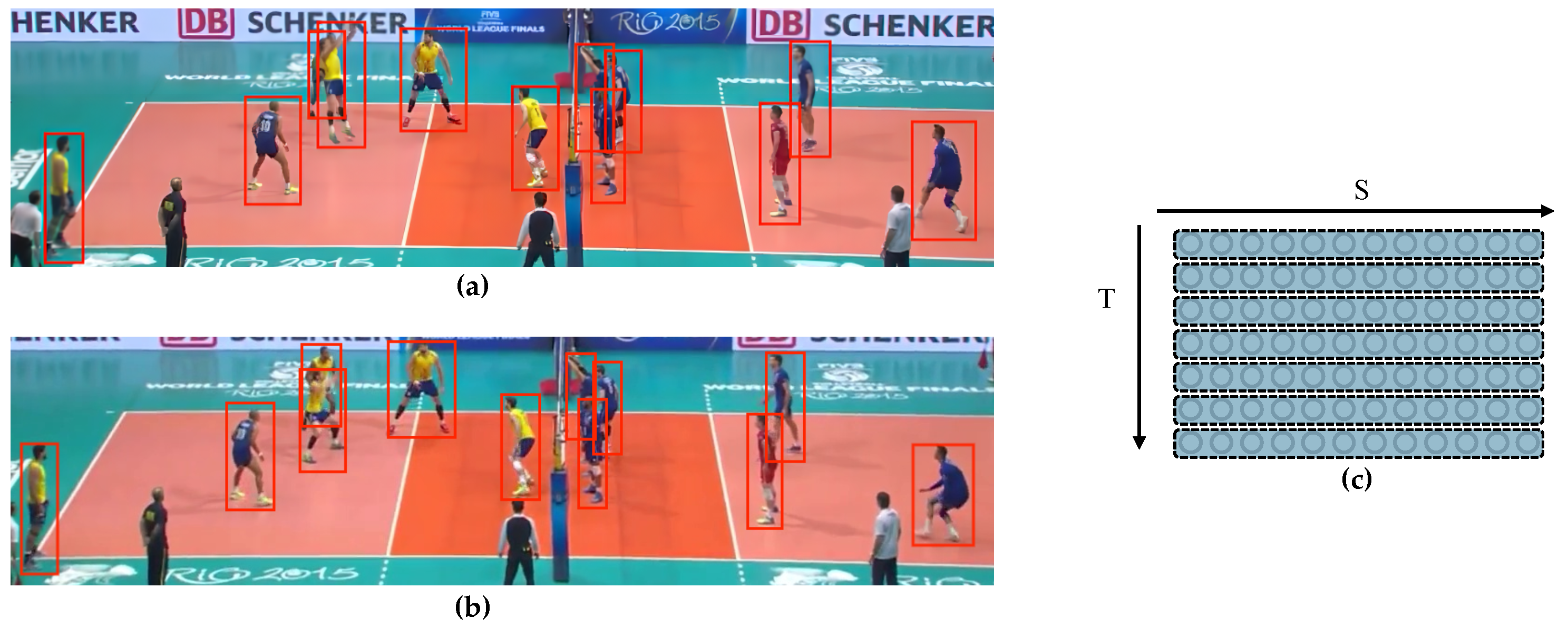
We also introduce constraints to further improve the performance of our network, i.e., global activity consistency and individual action consistency. First, the states of group activity in each frames should be similar to the states in other frames and have similar contribution to the recognition of the group activity. In other words, the features of the states of group activity in each frame in the same event video clip should be similar. The states of the same “set” (or set the ball) group activity in two frames are shown in Figure 3a,b. Since the states of the group activity in each frame should not change too much over time, the features of the states of group activity in each frame should have similar contributions to the recognition of the group activity. As shown in Figure 3c, each row or each grayed area represents a feature of the state of group activity in one frame, and all seven grayed areas should have similar features of the states of the group activity. We call this global activity consistency. Second, each individual action in the video clip should have similar contributions to the recognition of the group activity. Two individual actions in the same “set” group activity are shown in Figure 4a,b. Each corresponding player (each column or grayed area in Figure 4c) in the same video clip should have similar actions or features of individual actions. We call this individual action consistency. The consistency of individual actions also contributes to the recognition of the group activity.
We use contrastive learning to constrain the semantic contributions from the features of the states of group activity in each frame and the features of each individual action. This unique design of combining two one-dimensional global receptive fields allows our network to obtain global interactions more efficiently.
Our network was evaluated on two widely used datasets, the Volleyball dataset (VD) [14] and the Collective Activity dataset (CAD) [15]. Experimental results demonstrate that our network obtained superior classification accuracy with the lowest model complexity compared with the state-of-the-art networks.
Our contributions are summarized as follows:
(1) We propose a new global individual interaction network (GIIN) to model the interactions of all people in a group in the spatial–temporal domain. We design new convolution kernels to characterize the interactions of all people in a group activity from a global perspective.
(2) To avoid heavy computation when modeling global interactions, our proposed convolution kernels have two global receptive fields with one in the spatial dimension and another in the temporal dimension. They are connected in parallel to capture features of the group activity in a global sense without significantly increasing the computation cost.
(3) We employ the technique of contrastive learning to refine the features of the states of group activity in each frame and the features of each individual action.
(4) Experimental results show that the proposed network obtained comparable or better performance in terms of recognition accuracy with the lowest model complexity compared to the state-of-the-art networks.
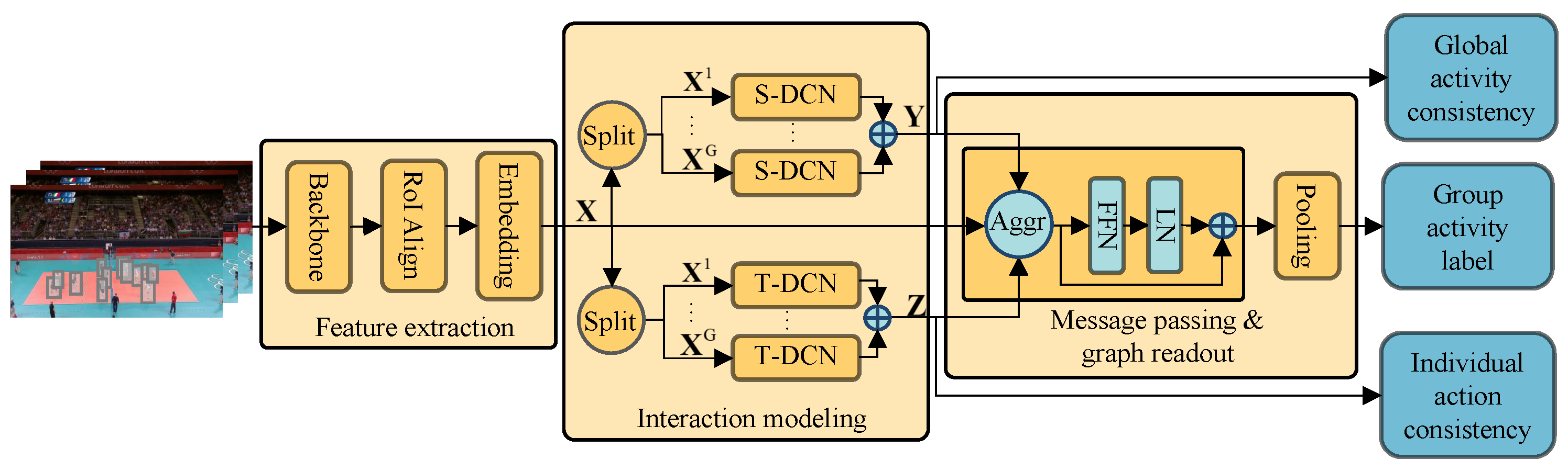
2. Related Work

2.1. Group Activity Recognition

Traditional GAR approaches only extract features at low abstract levels and are unable to represent the interactions among all people within a group activity. Early deep learning methods for GAR used the hierarchical temporal model to characterize the actions of individuals. However, it is a big task to accurately identify group activity by focusing only on the individual actions over time. Interactions among individuals in the entire group are important for GAR [1]. Recent research in this field attempts to improve the GAR performance by modeling the interactions in a group more efficiently.
Recent deep learning-based GAR methods [8,10,11,12,16,17,18,19,20] recognize the activity of a group in three steps. First, they encode the features of the states of each individual action in each frame in a video of a specific activity to obtain a feature map [21]. They then use a graph to describe the interactions among members within the group. The edges of the graph are obtained based on pre-defined or learnable interactions, and the attributes of each node are learned from the obtained feature map. Finally, they aggregate the features at the group level by pooling operations to recognize the group activity. Of these three steps, characterizing the interactions with an efficient model is important and has not been addressed successfully. While it has not been explicitly stated, MHSA-based methods [8,12] construct a fully connected graph with a spatial–temporal feature map, and then use self-attention as the weights of edges between pairs of nodes. The biggest challenge of MHSA-based methods is the high computational cost.
Graph neural networks (GNNs) have shown the ability to model interactions between nodes. GNN-based methods have attracted the attention of researchers in group activity recognition in recent years. Interactions among individuals are represented with predefined node connectivity (e.g., node distances) [11,12]. Computational cost for using predefined node connectivity is lower than using a fully connected graph, but it cannot be applied to node-specific interactions on the spatial–temporal feature map [13]. Inspired by the work of DCN [21,22], Yuan et al. designed a dynamic inference network (DIN) to effectively generate individual-specific dynamic interaction patterns on spatial–temporal graphs using random wandering to improve the recognition accuracy with a lower computational cost [13].
Since the GNN-based approaches use receptive field-confined convolutional or fully connected layers to characterize the local interactions that exist in a group activity video, they are not ideal for modeling the global interactions among individuals.

2.2. Contrastive Learning

Contrastive learning has been successively used for unsupervised learning in the domain of multi-view learning, which captures task-relevant information by maximizing the mutual information between features from different views [23]. The assumption in contrastive learning is that task-related information exists mainly in shared information between different views [24]. Contrastive learning learns the feature representation of a sample by comparing the data with positive and negative sample pairs in the feature space. The difficulty in contrastive learning lies in forming positive and negative sample pairs.
Motivated by its success in the field of multi-view learning, we use contrastive learning for GAR in this paper. Specifically, for the extracted features of the states of group activity in each frame and the features of each individual action, we learn the global activity consistency and individual action consistency respectively with contrastive learning to enable them to capture GAR-related information more efficiently.

3. Method

The framework of our proposed global individual interaction network (GIIN) consists of three main modules—the feature extraction module, the interaction modeling module, and the message passing and graph readout module—as shown in Figure 5.
We use the feature extraction module to extract the features of states of each individual action in each frame in the input video and construct a spatial–temporal feature map with the extracted features. In the interaction modeling module, we arrange the obtained feature map into a spatial–temporal graph and use our proposed convolutional kernels to extract the feature from a global perspective and update the interactions among individuals. We aggregate these features in the message passing and graph readout module and use them for GAR. We learn the global activity consistency and individual action consistency from the above features during training to capture more activity-relevant information.

3.1. Feature Extraction Module

In the feature extraction module as shown in Figure 5, we use ResNet-18 [25] as our backbone network to extract the features of each frame from the input video first. We crop the region features of individuals by RoIAlign [26]. We then reduce the channel dimension of the region features through an embedding layer to obtain the features of the states of each individual action in each frame. Here, we implement the embedding layer with a 1 × 1 convolution layer. To construct a spatial–temporal feature map X R C × S × T for the video, we stack the features of the states of each individual action in one frame from left to right according to the positions of the individuals in the x-axis of the image. We denote S as the number of people in each frame, T as the number of frames in the video, and C as the length of the feature of the state of an individual action in one frame. For frames that have fewer people than S, we follow the method used in [9,12,13] by replicating the available features of the states of individual actions along the spatial dimension until the entire row has features of the states of S individual actions. We repeat the same process for each frame in the temporal dimension.

3.2. Interaction Modeling

In this module, we first initialize a directed spatial–temporal graph with the feature map X , and then learn the spatial and temporal interactions in the spatial–temporal graph by using our proposed convolutional kernels in the T-DCN and S-DCN branches.
To construct a directed spatial–temporal graph based on the feature map of X , we regard each person in each frame as a node and treat the features of the states of each individual action in each frame as the attribute of the node. Thus, the constructed spatial–temporal graph contains S × T nodes, and the size of the attribute of each node is C. The edges of the graph represent the interaction between two people or nodes. For each node, we consider it a target node and initialize the corresponding source nodes according to the index difference in the spatial and temporal terms. We denote the nearest K nodes in the spatial dimension to each target node as its source nodes and the nearest K nodes in the temporal dimension as its source nodes so that each node is connected to 2 K source nodes through 2 K edges. Thus, the initialized spatial–temporal graph has S × T target nodes with K × S × T temporal edges and K × S × T spatial edges.
We use the weight of the edge to denote the importance of interaction between a source node and a target node, and use offset to denote the difference of positions between the updated source node and the initial source node. We learn the weights and offsets of spatial edges with the T-DCN branch and the weights and offsets of temporal edges with the S-DCN branch. Based on the learned offsets, we update the position of each source node by adding the offset to its initial position, and use weights to update the attribute of each node.
The constructed spatial–temporal graph characterizes the interactions among individuals in the group. However, the interactions that exist in a group activity are complicated because each individual (node) is influenced by its neighbors (adjacent nodes) dynamically. Previous methods [11,12,13] attempted to model the interactions among nodes by using mapping layers with local receptive fields in spatial–temporal dimensions and generate the model of individual interactions. Their ability to represent the spatial–temporal interactions is fairly limited because the local receptive fields can hardly capture global interaction patterns.
To overcome the above shortcoming, using a convolutional kernel with a larger receptive field is an intuitive approach, as it is more effective in capturing information unique to different locations. However, it comes with the burden of a larger number of parameters. We split a single 2-dimensional receptive field into two much simpler receptive fields to reduce the number of parameters. Specifically, we propose spatial global receptive field convolutional kernels (SGRF-Conv kernels) and temporal global receptive field convolutional kernels (TGRF-Conv kernels), respectively. The proposed SGRF-Conv kernels have global receptive fields in the spatial dimension and are grouped in the spatial dimension. Similarly, the TGRF-Conv kernels have global receptive fields in the temporal dimension and are grouped in the temporal dimension.

3.2.1. Operations of SGRF-Conv and TGRF-Conv

Suppose the input X is an order 3 tensor with size C × S × T . C, S and T denote the length of the channel, and the spatial and temporal dimensions of the input, respectively. The SGRF-Conv kernel is an order 3 tensor with size C × S × K , where C, S and K are the length of the channel, the spatial and the temporal dimensions, respectively. Please note that the SGRF-Conv kernel has the same length as the input in the spatial dimension to achieve a global receptive field of the spatial dimension as shown in Figure 2a. We construct the SGRF-Conv layer with D kernels of SGRF-Conv. We denote all the SGRF-Conv kernels in the SGRF-Conv layer as H R D × C × S × K . We use variables 1 d D , 1 c C , 1 i S , 1 u K and 1 j T to index elements in the kernels and the input.
The SGRF-Conv kernel is grouped in the spatial dimension when performing convolutional operations on the input. Figure 6a shows the result of the convolution operation between the input and the SGRF-Conv kernel. Since the convolution kernel has the same length as the input in the spatial dimension, it has a global receptive field in the spatial dimension and effectively reduces the number of parameters. We divide an SGRF-Conv kernel into S groups along the spatial dimension, and each group generates the corresponding output separately.
For simplicity, we set the stride to 1 and the padding to [ K / 2 ] (we use square brackets to indicate that K / 2 is rounded down). The output feature of SGRF-Conv is denoted as A , A R D × S × T . The SGRF-Conv operation can be expressed by Equation (1):
a d , i , j = c = 1 C u = 1 K h d , c , i , u x c , i , j + u + [ K / 2 ] ,
where x c , i , j + u + [ K / 2 ] is the element of X indexed by c , i , j + u + [ K / 2 ] , a d , i , j is the element of A indexed by d , i , j , and h d , c , i , u is the element of H indexed by d , c , i , u .
Similarly, suppose the input X is a three-order tensor in size of C × S × T . We design the TGRF-Conv kernel to be a three-order tensor with size C × K × T , where C, K and T are the length of the channel, the spatial and the temporal dimensions. The TGRF-Conv kernel has the same length as the input in the temporal dimension to achieve a global receptive field of the temporal dimension as shown in Figure 6b. We suppose that a TGRF-Conv layer contains D kernels of TGRF-Conv. We denote all TGRF-Conv kernels in the TGRF-Conv layer as F R D × C × K × T . We use index variables 1 d D , 1 c C , 1 j T , 1 v K and 1 i S to pinpoint a specific element in the kernels and the input.
For simplicity, we set the stride to 1 and padding to [ K / 2 ] . Hence, we have output in E R D × S × T . The TGRF-Conv operation can be expressed by Equation (2):
e d , i , j = c = 1 C v = 1 K f d , c , v , j x c , i + v + [ K / 2 ] , j ,
where x c , i + v + [ K / 2 ] , j is the element of X indexed by c , i + v + [ K / 2 ] , j , e d , i , j is the element of E indexed by d , i , j , f d , c , v , j is the element of F indexed by d , c , v , j .
Considering H is equipped with a global receptive field in the spatial dimension and F has a global receptive field in the temporal dimension, we use H and F to characterize the global interactions in the spatial–temporal dimensions. Moreover, we use group convolutions to reduce the number of parameters of our convolution kernels while providing more efficient receptive fields in the spatial–temporal dimensions.

3.2.2. S-DCN and T-DCN

In our method, each branch of S-DCN consists of two parallel SGRF-Conv layers (Figure 7), which learn the offsets and weights of the temporal edges, respectively. Similarly, each branch of T-DCN uses two TGRF-Conv layers to learn the offsets and weights of the spatial edges, respectively. With the offsets and weights of K temporal edges and K spatial edges of each target node, we can update the spatial–temporal graph and aggregate the features of each target node. Since the SGRF-Conv and TGRF-Conv operations have global receptive fields in the spatial dimension and temporal dimension respectively, the branches of S-DCN and T-DCN can characterize global interactions in the spatial–temporal dimensions.
Since each temporal edge has an offset and a weight, each graph corresponds to temporal offsets Δ P T R K × S × T and temporal weights M T R K × S × T . As is shown in Figure 7a, to obtain the temporal offset Δ P T and temporal weight M and update the relationship in the temporal dimension, we use two SGRF-Conv layers, i.e., H p R K × C × K × T and H m R K × C × K × T in S-DCN. The elements of Δ P T and M T can be calculated by Equations (3) and (4):
Δ p d , i , j T = c = 1 C u = 1 K h d , c , i , u p x c , i , j + u + [ K / 2 ] ,
m d , i , j T = c = 1 C u = 1 K h d , c , i , u m x c , i , j + u + [ K / 2 ] ,
where d = 1 , 2 , , K , and K is a hyperparameter and denotes the number of edges for each node in the temporal dimension. Δ p d , i , j T is the element of Δ P T indexed by d , i , j , m d , i , j T is the element of M T indexed by d , i , j , x c , i , j + u + [ K / 2 ] is the element of X indexed by c , i , j + u + [ K / 2 ] , h d , c , i , u p is the element of H p indexed by d , c , i , u , and h d , c , i , u m is the element of H m indexed by d , c , i , u . Please note that H p and H m are used to generate the offsets and weights with the same operation of SGRF-Conv as defined for H (please see Equation (1)). With the temporal offsets and temporal weights, we can update the temporal relationship and acquire the feature Y by Equation (5):
y : , i , j = d = 1 K W T m d , i , j T x : , i , j + [ d K / 2 ] + Δ p d , i , j T ,
where Y R C × S × T , W T R C × C is a learnable weight matrix, y : , i , j is a vector composed of all elements in Y with temporal dimension i and spatial dimension j, and x : , i , j + [ d K / 2 ] + Δ p d , i , j T is a vector composed of all elements in X with temporal dimension i and spatial dimension j + [ d K / 2 ] + Δ p d , i , j T . Y represents the feature of group activity to be aggregated in the temporal dimension and has the global interaction information in the spatial dimension since it is obtained from the SGRF-Conv operation. Since the index of the position must be an integer, while the offsets may be floating points, we follow the DCN presented in [22] and employ bilinear interpolation to generate the features of the source nodes, i.e.,
x : , i , j + [ d K / 2 ] + Δ p d , i , j T = j = 1 T i = 1 S x : , i , j max 0 , 1 j + [ d K / 2 ] + Δ p d , i , j T ,
where x : , i , j is a vector composed of all elements in X with temporal dimension i and spatial dimension j.
Similarly, to obtain the spatial offsets Δ P S and spatial weights M S , we use two TGRF-Conv layers, i.e., F p and F m in T-DCN as shown in Equations (7) and (8):
Δ p d , i , j S = c = 1 C v = 1 K f d , c , v , j p x c , i + v + [ K / 2 ] , j ,
m d , i , j S = c = 1 C v = 1 K f d , c , v , j m x c , i + v + [ K / 2 ] , j ,
where F p R K × C × K × T and F m R K × C × K × T . Δ p d , i , j S is the element of Δ P S indexed by d , i , j , m d , i , j S is the element of M S indexed by d , i , j , x c , i + v + [ K / 2 ] , j is the element of X indexed by c , i + v + [ K / 2 ] , j , f d , c , v , j p is the element of F p indexed by d , c , v , j , and f d , c , v , j m is the element of F m indexed by d , c , v , j . Then, we can update the spatial relationship and acquire feature Z R C × S × T by Equations (9) and (10):
x : , i + [ d K / 2 ] + Δ p d , i , j S , j = j = 1 T i = 1 S x : , i , j max 0 , 1 i + [ d K / 2 ] + Δ p d , i , j S ,
z : , i , j = d = 1 K W S m d , i , j S x : , i + [ d K / 2 ] + Δ p d , i , j S , j ,
where W S R C × C is a learnable weight matrix different from W T in Equation (5), x : , i , j is a vector composed of all elements in X with temporal dimension i and spatial dimension j, x : , i + [ d K / 2 ] + Δ p d , i , j S , j is a vector composed of all elements in X with temporal dimension i + [ d K / 2 ] + Δ p d , i , j S and spatial dimension j. z : , i , j is a vector composed of all elements in Z with temporal dimension i and spatial dimension j, and Z represents the feature of group activity to be aggregated in the spatial dimension and has the global interaction information in the temporal dimension since it is obtained from TGRF-Conv operation.
As shown in Figure 5, to characterize the interactions efficiently, we split X into G groups along the channel dimension, and denote the g-th group of X as X g R ( C / G ) × S × T , g = 1 , 2 , , G . Then we initialize the T-DCN and S-DCN branches of G, respectively, and feed X g , g = 1 , 2 , , G into the g-th S-DCN and g-th T-DCN without shared parameters. We denote the output of the g-th S-DCN as Y g and the output of the g-th T-DCN as Z g . We can acquire the temporal offsets and temporal weights of X g by Equations (3) and (4). We set the size of the learnable weight matrix in Equation (5) to ( C / G ) × C to ensure that the channels of Y g are the same size as the original channels. Finally, we sum up Y g , g = 1 , 2 , , G to acquire Y . Similarly, we set the size of the learnable weight matrix in Equation (10) to ( C / G ) × C to ensure that the channels of the output Z g are the same size as the original channels. We sum up Z g , g = 1 , 2 , , G to acquire Z .
The summary of S-DCN and T-DCN is shown in Table 1.

3.3. Message Passing and Graph Readout Module

In the message passing and graph readout module, we aggregate X , Y and Z to update the attributes of each node. Specifically, we use the summation–aggregation to update the features of each target node with X , Y and Z . We use Equation (11) to aggregate Y and Z . Then we use a 2-layer 1×1 convolution in the feed forward network (FFN) to refine the aggregated features X ˜ as shown in Equation (12):
X ˜ = σ [ ( Y + Z ) / 2 ] + X ,
X ˜ ˜ = D r o p o u t ( F F N ( X ˜ ) + X ˜ ) ,
where X ˜ ˜ is the refined feature. Finally, we perform pooling and linear mapping on X ˜ ˜ to acquire group activity labels c l s . We use the cross entropy to calculate classification loss L cls by Equation (13):
L cls = C r o s s E n t r o p y ( c l s ^ , c l s ) ,
where c l s is the ground truth of the group activity.

3.4. Global Activity Consistency and Individual Action Consistency Learning

We use T-DCN branches and S-DCN branches to capture the activity-relevant information more efficiently by maximizing the consistency of the features of the states of group activity in each frame and the consistency of features of individual actions, i.e., the global activity consistency and individual action consistency. We first construct positive and negative sample pairs, and then follow the routine of contrast learning [27] to constrain the similarity of the constructed sample pairs. Supposing that a and b are feature vectors of two samples, we use Equation (14) to measure the similarity between them,    
S τ ( a , b ) = exp a , b a b 1 τ ,
where τ is a hyperparameter. Specifically, suppose there are B samples in each mini-batch input into GIIN. We denote the feature samples obtained from the S-DCN branches as Y 1 , . . . Y b , . . . Y B , where Y b , where Y b represents the feature of the group activity with global interaction information in the spatial dimension of the b-th video in the mini-batch. Then, we slice each Y b , b = 1 , 2 , , B into T slices along the temporal dimension, and denote them as Y : , : , 1 b , . . . , Y : , : , j b , . . . , Y : , : , T b . Y b : , : , j represents the features of the states of group activity of the b-th sample at the j-th frame. Since Y b : , : , j is obtained from SGRF-Conv, it provides global interaction information in the spatial dimension. To maximize the consistency of the features of the states of group activity in each frame, we construct positive and negative sample pairs at the training stage. As shown in Figure 8a, we consider the features of the states of group activity learned from the same video as positive sample pairs, and the features of the states of group activity learned from different videos in the same mini-batch as the negative sample pairs.
We use Equation (15) as the loss function for global activity consistency learning. The numerator in Equation (15) represents the similarity between the features of two states of group activity in a positive sample pair, and the sum term in the denominator indicates the similarity between the features of two states of group activity in the negative sample pairs. To decrease the loss of global activity consistency learning, we want the similarity for positive sample pairs as large as possible and the similarity for negative sample pairs as small as possible:
L group = b = 1 B j = 1 T r = 1 r j T log S τ Y : , : , j b , Y : , : , r b S τ Y : , : , j b , Y : , : , r b + a = 1 a b B e = 1 T S τ Y : , : , j b , Y : , : , e a
Similar to the global activity consistency learning, suppose there are B samples in each mini-batch input into GIIN; we denote the feature samples obtained from the T-DCN branches as Z 1 , . . . Z b , . . . Z B , where Z b represents the feature of group activity with global interaction information in the temporal dimension of the b-th video in the mini-batch. Then, we slice each Z b , b = 1 , 2 , , B in the mini-batch into S slices along the spatial dimension, and denote them as Z : , 1 , : b , . . . , Z : , i , : b , . . . , Z : , S , : b . Z : , i , : represents the feature of individual actions of the b-th sample for the i-th person. Since Z : , i , : is obtained from TGRF-Conv, it provides global interaction information in the temporal dimension. To maximize the consistency of the features of individual actions, we construct positive and negative sample pairs at the training stage (Figure 8b). We consider the features of individual actions learned from the same Z b as positive sample pairs, and the features of individual actions from different videos in the same batch as negative sample pairs. Then, we use Equation (16) as the loss for individual action consistency:
L individual = b = 1 B i = 1 S q = 1 q i S log S τ Z : , i , : b , Z : , q , : b S τ Z : , i , : b , Z : , q , : b + a = 1 a b B f = 1 T S τ Z : , i , : b , Z : , f , : a
Finally, we combine all the losses to train our GIIN as shown in Equation (16):
L = L cls + β ( L group + L individual )
where β is a hyperparameter. We perform end-to-end training using Equation (17) to learn effective features with constraints of global activity consistency and individual action consistency.
Our algorithm is shown in Algorithm 1. Electronics 12 04104 i001

4. Experiment

In this section, we discuss the evaluation performance of our proposed method on two widely used datasets. We first introduce the datasets and implementation details. Then we compare the proposed method (GIIN) with the state-of-the-art GAR approaches in terms of accuracy and computational complexity. We also analyze GIIN from the perspective of confusion matrices and conduct ablation studies to investigate the effectiveness of the interaction modeling module and consistency learning constraints.

4.1. Experiment Settings

4.1.1. Datasets

We carried out experiments on two datasets: the Volleyball dataset (VD) [14] and the Collective Activity dataset (CAD) [15]. These two datasets are publicly available and widely used in the research of group activity recognition [11,12]. Other action video datasets, such as NTU RGB+D [28], Kinetics [29], UCF101 [30], HMDB51 [31], and ActivityNet [32], are also important, but these datasets were constructed specifically for individual action recognition. The action videos in these datasets lack interactive information among individuals and do not include group activity labels. For these reasons, the mainstream GAR methods and our method cannot be evaluated on these human action datasets.
The Volleyball dataset consists of 3493 training clips and 1337 testing clips trimmed from 55 volleyball game videos. Each clip sample provides three types of annotations, including the label of group activity, the coordinates of the bounding box for individuals, and the labels for individual actions. The labels of group activity consist of r i g h t s e t , r i g h t s p i k e , r i g h t p a s s , r i g h t w i n p o i n t , l e f t s e t , l e f t s p i k e , l e f t p a s s , and l e f t w i n p o i n t . The labels of individual actions were not used in our experiments.
The Collective Activity dataset consists of 44 videos. The length of video ranges from 194 to 1814 frames. Each video of the Collective Activity dataset also has three types of annotations, including the coordinates of the person’s bounding box for the center frame every ten frames, the group activity labels ( c r o s s i n g , w a i t i n g , q u e u i n g , w a l k i n g , and t a l k i n g ) every ten frames, and the individual action labels. The individual action labels were not used in our experiments. We followed the routines of [20] to split the data into the training set and test set. We also followed [8,11,13] to merge the samples of c r o s s i n g and w a l k i n g into m o v i n g .
We followed MLST-Former [33] and DIN [13] and used multi-class classification accuracy (MCA) and mean per class accuracy (MPCA) to evaluate the classification performance of the compared models. We used the number of parameters (#Params) and FLOPs to evaluate the complexity of the compared models. In the test set, we denote the number of samples in the k-th class as p k , k = 1 , 2 , , K , where K is the number of classes, and the number of correctly recognized samples in the k-th class is q k . The calculations of MCA and MPCA are formulated as Equations (18) and (19):
M C A = k = 1 K q k k = 1 K p k
M P C A = 1 K k = 1 K q k p k

4.1.2. Details of Implementation

The resolutions of the video frame were 720 × 1280 for VD and 480 × 720 for CAD. We set T = 10 frames per video clip. The maximum number of people (S) in the scene was set to 12 for the VD and 13 for the CAD. The embedded dimension of the person features C was set to 128. The SGRF-Conv and TGRF-Conv kernels used by GIIN were initialized as zero vectors. In the process of graph convolution, we used zero padding to maintain a fixed number of edges for each node. We followed the routines in [12,13] and initialized the backbone of the GIIN model with the parameters of [12], and the implementation of consistent learning was based on the code of CMC [23]. We did not use individual action labels as supervision for the network training. In the training on both VD and CAD, we used the Adam optimizer and OneCycleLR [34] scheduler with learning rates from 1 × 10 4 to 3 × 10 4 and trained 25 epochs. The hyperparameters of Adam were β 1 = 0.9 , β 2 = 0.999 , and ϵ = 10 7 . The hyperparameters of OneCycleLR were div_factor = 3, pct_start = 0.3, final_div_factor = 2 and three_phase = True. We used β = 10 6 for VD and β = 10 4 for CAD. The numbers of edges in the T-DCN and S-DCN were set as K = 3 and G = 4. We used ResNet-18 as the backbone of the compared methods in the experiments.

4.2. Comparisons with the State-of-the-Art Methods

To demonstrate the improved performance of our method, we compared our method with the state-of-the-art methods in terms of classification accuracy and complexity on VD and CAD. Table 2 shows the comparison results on VD between our method and the non-MHSA-based methods, including GNN-based methods and hierarchical temporal models, in terms of classification accuracy (MCA and MPCA) and model complexity. All the compared methods used RGB video clips as input, and the ResNet-18 was used as the backbone for these methods. To have a fair comparison, we followed the method employed in [13] and evaluated the number of parameters (i.e., #Params) and FLOPs without counting the backbone and embedding layer in Table 2. For reference, we also present the number of parameters and FLOPs for the backbone and the embedding layer: 24.302 M #Params, 676.364 GFLOPs for 720 × 1280 resolution.
Table 2 shows that our method achieved the highest MCA and MPCA with the lowest #Params and FLOPS on the VD using the same backbone and RGB input conditions. Specifically, compared with the previous GNN-based methods, our method obtained the highest recognition accuracy. The #Params of our model without the backbone and the embedding layer is only 30% of DIN [13], and the FLOPS is only 23% of DIN [13]. These results show the efficiency of our GAR method. We attribute the efficiency of our method to two reasons. On one hand, since the convolutional kernels we used have a global receptive field and are grouped in the spatial or temporal dimension, our proposed method characterizes the global interactions among individuals with a limited number of parameters. On the other hand, activity-relevant information was effectively characterized by introducing constraints on global activity and individual action consistencies.
In Table 3, we compare the classification performance and model complexity between our method and the MHSA-based methods on the VD. Since MLST-Former [33] calculated the #Params and FLOPs of the backbone and embedding layers in a different way, we recalculated the total #Params and total FLOPs according to MLST-Former [33].
The results in Table 3 show that, compared to MHSA-based methods, our method obtained comparable classification accuracy with significantly lower complexity. Specifically, although our method obtained a slightly lower MCA(0.9%) compared with the MLST-Former [33], the #Params of our interaction modeling module is only 17.1% of MLST-Former [33], and the FLOPs is only 3.9% of MLST-Former [33]. The above results show that our method is efficient compared to the MHSA-based methods.
GroupFormer [10] obtained the best performance in terms of MCA mostly because it requires the RGB video, optical flow and individual poses. Compared to GroupFormer, our proposed method only requires input from RGB video clips, and obtained comparable MCA with only 0.6% parameters and (0.4%) FLOPs of GroupFormer.
We compared our proposed method with the state-of-the-art methods in terms of MCA and MPCA on the CAD. As shown in Table 4, our method achieved the highest MCA and MPCA on CAD. Specifically, the MCA of our method is 1.2% higher than GroupFormer [10], even though it requires RGB video clips, optical flow, and individual pose as input. Compared with MLST-Former [33], which obtained the highest MCA among all the previous methods, our method performed 0.7% better in terms of MCA. Compared with Dual-AI [8], which achieved the highest MPCA among all the previous methods, our method performed 0.6% better in terms of MPCA.
The above results show the improved performance of our method on the CAD. We attribute the highest recognition accuracy of our method to the proposed S-DCN and T-DCN branches and the consistency learning constraints based on global activity and individual action consistencies.

4.3. Confusion Analysis and Experimental Curves

Figure 9a,b show the confusion matrices of our proposed method on the VD and CAD, respectively. As shown in Figure 9a, GIIN achieved over 90% recognition accuracy for all classes on VD except r i g h t   s e t . In particular, the recognition accuracy of GIIN for r i g h t   w i n p o i n t and l e f t   w i n p o i n t exceeded 97%. The above results show that GIIN can well distinguish different activities, especially left and right activities. Misclassified cases were mainly from the samples for s e t , p a s s and s p i k e , which may be because individuals who provide critical clues for these three types of group activities show highly similar actions. As shown in Figure 9b, GIIN achieved over 90% recognition accuracy for all classes on CAD. In particular, the recognition accuracy of GIIN in terms of m o v i n g , q u e u i n g and t a l k i n g was above 98%. Since the difference between w a i t i n g and q u e u e i n g is the movement of the human body in the temporal dimension, it is important to effectively characterize temporal interactions from a global perspective. The above result suggests that our method achieved accurate recognition by effectively modeling temporal interactions from a global perspective. Our misclassification mainly occurred when identifying w a i t i n g and m o v i n g , which most likely resulted from the two types of activities being similar and the temporal dynamic of the samples being too short [17].
The classification loss curves in training and classification performance curves in testing are included to show the loss and the network performance for different epochs. Figure 10a,d show that the classification losses converge to a lower level after 15 epochs on VD and 20 epochs on CAD, while the performance of our method gradually improves until it is convergent after 15 epochs on VD and 20 epochs on CAD, as shown in Figure 10b,c,e,f. Because we initialized the backbone of our proposed method with the parameters pre-trained on [12], our model converges fairly quickly.

4.4. Ablation Studies

We performed ablation experiments on VD and CAD to validate the effectiveness of the interaction modeling module and consistency learning constraints. We used MCA and MPCA as evaluation metrics. We constructed three networks for the ablation experiments, namely the base model, GIIN w/o contrast, and GIIN. The base model includes the feature extraction module, the pooling layer, and the classification layers in the graph readout module. We used the experimental results of the base model as the baseline performance. The network of GIIN w/o contrast contains the feature extraction module, interaction modeling module, and message passing and graph readout module but does not contain consistency learning. The network of GIIN is shown in Figure 5, and contains the feature extraction module, interaction modeling module, message passing and graph readout module, and global activity and individual action consistencies learning.
The experiment results on VD and CAD are shown in Table 5. Compared with the base model, GIIN w/o contrast improves MCA by 0.9% and MPCA by 1.0% on the VD, and improves MCA by 2.7% and MPCA by 4.4% on the CAD. The results show the efficiency of our proposed S-DCN and T-DCN in GAR. Compared with the GIIN w/o contrast, GIIN improves MCA by 1.5% and MPCA by 1.5% on the VD, and improves MCA by 1.3% and MPCA by 2% on the CAD. Since GIIN only adds the constraints of consistency learning compared with GIIN w/o contrast, we attribute the above results to the constraints on global activity and individual action consistencies, which help the network effectively capture the information for the GAR task.

5. Conclusions

In this paper, we propose a global individual interaction network based on global interaction modeling and the constraints of global activity and individual action consistencies. Our method addresses the problem that previous GNN-based GAR methods characterize the interactions locally with mapping layers using local receptive fields. We design SGRF-Conv and TGRF-Conv convolutions to provide global receptive fields in the spatial and temporal dimensions efficiently. At the same time, we construct constraints of global activity and individual action consistencies based on contrastive learning to characterize GAR features. Experimental results show that, compared with the state-of-the-art methods, the proposed method obtained better performance in terms of MCA and MPCA, and with a lower computational cost.

Author Contributions

Conceptualization, C.H. and D.Z.; methodology, C.H. and D.Z.; software, C.H. and Y.X.; validation, C.H., B.L. and Y.X.; formal analysis, C.H. and D.Z.; investigation, C.H., B.L., Y.X., D.Z. and D.-J.L.; resources, C.H. and D.Z.; data curation, C.H. and D.Z.; writing—original draft preparation, C.H. and D.Z.; writing—review and editing, D.Z. and D.-J.L.; visualization, C.H. and Y.X.; supervision, D.Z. and D.-J.L.; project administration, D.Z.; funding acquisition, D.Z. All authors have read and agreed to the published version of the manuscript.

Funding

This work was supported by the National Natural Science Foundation of China (62173353), Science and Technology Program of Guangzhou, China (202007030011).

Institutional Review Board Statement

Not applicable.

Informed Consent Statement

Not applicable.

Data Availability Statement

The Volleyball dataset(VD) is accessible at GitHub, https://github.com/mostafa-saad/deep-activity-rec#dataset (accessed on 11 September 2023). The Collective Activity dataset(CAD) is accessible at https://cvgl.stanford.edu/projects/collective/collectiveActivity.html (accessed on 11 September 2023). The data generated during the current study are available from the corresponding author on reasonable request.

Conflicts of Interest

The authors declare no conflict of interest.

References

  1. Wu, L.-F.; Wang, Q.; Jian, M.; Qiao, Y.; Zhao, B.-X. A comprehensive review of group activity recognition in videos. Int. J. Autom. Comput. 2021, 18, 334–350. [Google Scholar] [CrossRef]
  2. Aquino, G.; Costa, M.G.; Costa Filho, C.F. Explaining one-dimensional convolutional models in human activity recognition and biometric identification tasks. Sensors 2022, 22, 5644. [Google Scholar] [CrossRef] [PubMed]
  3. Wu, Y.-C.; Chen, C.-H.; Chiu, Y.-T.; Chen, P.-W. Cooperative people tracking by distributed cameras network. Electronics 2021, 10, 1780. [Google Scholar] [CrossRef]
  4. Huang, Q.; Hao, K. Development of cnn-based visual recognition air conditioner for smart buildings. J. Inf. Technol. Constr. 2020, 25, 361–373. [Google Scholar] [CrossRef]
  5. Amer, M.R.; Lei, P.; Todorovic, S. Hirf: Hierarchical random field for collective activity recognition in videos. In Computer Vision–ECCV 2014: 13th European Conference, Zurich, Switzerland, September 6-12, 2014, Proceedings, Part VI 13; Springer International Publishing: Cham, Switzerland, 2014; pp. 572–585. [Google Scholar]
  6. Lan, T.; Sigal, L.; Mori, G. Social roles in hierarchical models for human activity recognition. In Proceedings of the 2012 IEEE Conference on Computer Vision and Pattern Recognition, Providence, RI, USA, 16–21 June 2012; pp. 1354–1361. [Google Scholar]
  7. Choi, W.; Shahid, K.; Savarese, S. Learning context for collective activity recognition. In Proceedings of the CVPR 2011, Colorado Springs, CO, USA, 20–25 June 2011; pp. 3273–3280. [Google Scholar]
  8. Han, M.; Zhang, D.J.; Wang, Y.; Yan, R.; Yao, L.; Chang, X.; Qiao, Y. Dual-ai: Dual-path actor interaction learning for group activity recognition. In Proceedings of the IEEE/CVF Conference on Computer Vision and Pattern Recognition, New Orleans, LA, USA, 19–24 June 2022; pp. 2990–2999. [Google Scholar]
  9. Gavrilyuk, K.; Sanford, R.; Javan, M.; Snoek, C.G. Actor-transformers for group activity recognition. In Proceedings of the IEEE/CVF Conference on Computer Vision and Pattern Recognition, Seattle, WA, USA, 14–19 June 2020; pp. 839–848. [Google Scholar]
  10. Li, S.; Cao, Q.; Liu, L.; Yang, K.; Liu, S.; Hou, J.; Yi, S. Groupformer: Group activity recognition with clustered spatial-temporal transformer. In Proceedings of the IEEE/CVF International Conference on Computer Vision, Montreal, BC, Canada, 11–17 October 2021; pp. 13668–13677. [Google Scholar]
  11. Yan, R.; Xie, L.; Tang, J.; Shu, X.; Tian, Q. Higcin: Hierarchical graph-based cross inference network for group activity recognition. IEEE Trans. Pattern Anal. Mach. Intell. 2020, 45, 6955–6968. [Google Scholar] [CrossRef] [PubMed]
  12. Wu, J.; Wang, L.; Wang, L.; Guo, J.; Wu, G. Learning actor relation graphs for group activity recognition. In Proceedings of the IEEE/CVF Conference on Computer Vision and Pattern Recognition, Long Beach, CA, USA, 15–20 June 2019; pp. 9964–9974. [Google Scholar]
  13. Yuan, H.; Ni, D.; Wang, M. Spatio-temporal dynamic inference network for group activity recognition. In Proceedings of the IEEE/CVF International Conference on Computer Vision, Montreal, BC, Canada, 11–17 October 2021; pp. 7476–7485. [Google Scholar]
  14. Ibrahim, M.S.; Muralidharan, S.; Deng, Z.; Vahdat, A.; Mori, G. A hierarchical deep temporal model for group activity recognition. In Proceedings of the IEEE Conference on Computer Vision and Pattern Recognition, Las Vegas, NV, USA, 27–30 June 2016; pp. 1971–1980. [Google Scholar]
  15. Choi, W.; Shahid, K.; Savarese, S. What are they doing?: Collective activity classification using spatio-temporal relationship among people. In Proceedings of the 2009 IEEE 12th International Conference on Computer Vision Workshops, ICCV Workshops, Kyoto, Japan, 27 September–4 October 2009; pp. 1282–1289. [Google Scholar]
  16. Pramono, R.R.A.; Chen, Y.T.; Fang, W.H. Empowering relational network by self-attention augmented conditional random fields for group activity recognition. In Proceedings of the European Conference on Computer Vision, Glasgow, UK, 23–28 August 2020; pp. 71–90. [Google Scholar]
  17. Yuan, H.; Ni, D. Learning visual context for group activity recognition. In Proceedings of the AAAI Conference on Artificial Intelligence, Virtual, 2–9 February 2021; Volume 35, pp. 3261–3269. [Google Scholar]
  18. Wu, Z.; Pan, S.; Long, G.; Jiang, J.; Zhang, C. Graph wavenet for deep spatial-temporal graph modeling. arXiv 2019, arXiv:1906.00121. [Google Scholar]
  19. Zhou, H.; Kadav, A.; Shamsian, A.; Geng, S.; Lai, F.; Zhao, L.; Liu, T.; Kapadia, M.; Graf, H.P. Composer: Compositional reasoning of group activity in videos with keypoint-only modality. In Proceedings of the European Conference on Computer Vision, Tel Aviv, Israel, 23–27 October 2022; pp. 249–266. [Google Scholar]
  20. Qi, M.; Qin, J.; Li, A.; Wang, Y.; Luo, J.; Van Gool, L. stagnet: An attentive semantic rnn for group activity recognition. In Proceedings of the European Conference on Computer Vision (ECCV), Munich, Germany, 8–14 September 2018; pp. 101–117. [Google Scholar]
  21. Zhang, L.; Xu, D.; Arnab, A.; Torr, P.H. Dynamic graph message passing networks. In Proceedings of the IEEE/CVF Conference on Computer Vision and Pattern Recognition, Seattle, WA, USA, 14–19 June 2020; pp. 3726–3735. [Google Scholar]
  22. Dai, J.; Qi, H.; Xiong, Y.; Li, Y.; Zhang, G.; Hu, H.; Wei, Y. Deformable convolutional networks. In Proceedings of the IEEE International Conference on Computer Vision, Venice, Italy, 22–29 October 2017; pp. 764–773. [Google Scholar]
  23. Tian, Y.; Krishnan, D.; Isola, P. Contrastive multiview coding. In Computer Vision–ECCV 2020: 16th European Conference, Glasgow, UK, August 23–28, 2020, Proceedings, Part XI 16; Springer: Cham, Switzerland, 2020; pp. 776–794. [Google Scholar]
  24. Sridharan, K.; Kakade, S.M. An information theoretic framework for multi-view learning. In Proceedings of the Annual Conference Computational Learning Theory, Helsinki, Finland, 9–12 July 2008. [Google Scholar]
  25. He, K.; Zhang, X.; Ren, S.; Sun, J. Deep residual learning for image recognition. In Proceedings of the IEEE Conference on Computer Vision and Pattern Recognition, Las Vegas, NV, USA, 27–30 June 2016; pp. 770–778. [Google Scholar]
  26. He, K.; Gkioxari, G.; Dollár, P.; Girshick, R. Mask r-cnn. In Proceedings of the IEEE International Conference on Computer Vision, Venice, Italy, 22–29 October 2017; pp. 2961–2969. [Google Scholar]
  27. Oord, A.v.d.; Li, Y.; Vinyals, O. Representation learning with contrastive predictive coding. arXiv 2018, arXiv:1807.03748. [Google Scholar]
  28. Shahroudy, A.; Liu, J.; Ng, T.-T.; Wang, G. Ntu rgb+ d: A large scale dataset for 3d human activity analysis. In Proceedings of the IEEE Conference on Computer Vision and Pattern Recognition, Las Vegas, NV, USA, 27–30 June 2016; pp. 1010–1019. [Google Scholar]
  29. Kay, W.; Carreira, J.; Simonyan, K.; Zhang, B.; Hillier, C.; Vijayanarasimhan, S.; Viola, F.; Green, T.; Back, T.; Natsev, P.; et al. The kinetics human action video dataset. arXiv 2017, arXiv:1705.06950. [Google Scholar]
  30. Soomro, K.; Zamir, A.R.; Shah, M. Ucf101: A dataset of 101 human actions classes from videos in the wild. arXiv 2012, arXiv:1212.0402. [Google Scholar]
  31. Kuehne, H.; Jhuang, H.; Garrote, E.; Poggio, T.; Serre, T. Hmdb: A large video database for human motion recognition. In Proceedings of the 2011 International Conference on Computer Vision, Sophia Antipolis, France, 20–22 September 2011; pp. 2556–2563. [Google Scholar]
  32. Caba Heilbron, F.; Escorcia, V.; Ghanem, B.; Carlos Niebles, J. Activitynet: A large-scale video benchmark for human activity understanding. In Proceedings of the IEEE Conference on Computer Vision and Pattern Recognition, Boston, MA, USA, 7–12 June 2015; pp. 961–970. [Google Scholar]
  33. Zhu, X.; Zhou, Y.; Wang, D.; Ouyang, W.; Su, R. Mlst-former: Multi-level spatial-temporal transformer for group activity recognition. IEEE Trans. Circuits Syst. Video Technol. 2022, 33, 3383–3397. [Google Scholar] [CrossRef]
  34. Smith, L.N.; Topin, N. Super-convergence: Very fast training of neural networks using large learning rates. In Proceedings of the Artificial Intelligence and Machine Learning for Multi-Domain Operations Applications, SPIE, Baltimore, MD, USA, 10 May 2019; Volume 11006, pp. 369–386. [Google Scholar]
  35. Yan, R.; Tang, J.; Shu, X.; Li, Z.; Tian, Q. Participation-contributed temporal dynamic model for group activity recognition. In Proceedings of the 26th ACM international conference on Multimedia, Seoul, Republic of Korea, 22–26 October 2018; pp. 1292–1300. [Google Scholar]
  36. Shu, T.; Todorovic, S.; Zhu, S.-C. Cern: Confidence-energy recurrent network for group activity recognition. In Proceedings of the IEEE Conference on Computer Vision and Pattern Recognition, Honolulu, HI, USA, 21–26 July 2017; pp. 5523–5531. [Google Scholar]
  37. Bagautdinov, T.; Alahi, A.; Fleuret, F.; Fua, P.; Savarese, S. Social scene understanding: End-to-end multi-person action localization and collective activity recognition. In Proceedings of the IEEE Conference on Computer Vision and Pattern Recognition, Honolulu, HI, USA, 21–26 July 2017; pp. 4315–4324. [Google Scholar]
  38. Hu, G.; Cui, B.; He, Y.; Yu, S. Progressive relation learning for group activity recognition. In Proceedings of the IEEE/CVF Conference on Computer Vision and Pattern Recognition, Seattle, WA, USA, 14–19 June 2020; pp. 980–989. [Google Scholar]
Figure 1. (a) The local receptive field and (b) global receptive field in both S (spatial) and T (temporal) dimensions that is used as the mapping layers of the existing GNN-based group activity recognition methods.
Electronics 12 04104 g001
Figure 2. The new mapping layers with (a) a global receptive field in S and a local receptive field in T, and (b) a local receptive field in S and a global receptive field in T.
Electronics 12 04104 g002
Figure 3. (a,b) Two frames from the “set” group activity. (c) The features of states of group activity in each frames represented by each row should have similar contribution to the recognition of the overall group activity.
Electronics 12 04104 g003
Figure 4. (a,b) Two individual actions of the “set” group activity. (c) Features of individual actions represented by each column should be similar and have similar contributions to the recognition of the overall group activity.
Electronics 12 04104 g004
Figure 5. The framework of GIIN.
Electronics 12 04104 g005
Figure 6. Illustration of the input and output of (a) SGRF-Conv kernel and (b) TGRF-Conv kernel. We use different colors to indicate that the input values at different spatial or temporal positions are convolved to obtain the corresponding output values of the same color. The SGRF-Conv kernel slides the window in the temporal dimension, and the TGRF-Conv kernel slides the window in the spatial dimension. The size of the output in (a,b) are both S × T .
Electronics 12 04104 g006
Figure 7. The structures of the (a) S-DCN and (b) T-DCN.
Electronics 12 04104 g007
Figure 8. The process of constructing positive and negative sample pairs for consistency learning. Y 1 , . . . Y b , . . . Y B and Z 1 , . . . Z b , . . . Z B are the features of group activity obtained through the branches of S-DCN and T-DCN in a mini-batch. (a) The process of constructing positive and negative sample pairs for global activity consistency learning. We slice Y b , b = 1 , 2 , , B , along the temporal dimension. (b) The process of constructing positive and negative sample pairs for individual action consistency learning. We slice Z b , b = 1 , 2 , , B along the spatial dimension.
Electronics 12 04104 g008
Figure 9. The confusion matrix for (a) VD and (b) CAD.
Electronics 12 04104 g009
Figure 10. The classification loss curves in training and the classification performance curves in testing. (a,d) are the classification loss curves in training on VD and CAD respectively. (b,c) are the MCA and MPCA curves on VD in testing, while (e,f) are the MCA and MPCA curves on CAD in testing.
Electronics 12 04104 g010
Table 1. Summary of S-DCN and T-DCN.
Parameter Sharing DimensionThe Direction of the Sliding WindowDimensions of the Generated Aggregation
S-DCNTimeTimeTime
T-DCNSpaceSpaceSpace
Table 2. Comparisons with the non-MHSA-based methods on the VD The number of parameters and FLOPs of the backbone and the embedding layer are not included. The best result is highlighted in bold.
MethodVD MCA(%)VD MPCA(%)#ParamsFLOPS
PCTDM [35]90.390.526.235 M6.298 G
ARG [12]91.191.425.182 M5.436 G
HiGCIN [11]91.492.01.051 M184.992 G
SACRF [16]90.79129.422 M76.757 G
DIN [13]93.193.31.305 M0.311 G
Ours93.694.20.394 M0.070 G
Table 3. Comparisons with the MHSA-based methods on the VD. The number of parameters and FLOPs for the backbone and the embedding layer are not included. The best result is highlighted in bold.
MethodVD MCA(%)#ParamsFLOPsTotal #ParamsTotal FLOPs
AT [9]905.245 M1.260 G29.547 M677.624 G
GroupFormer 1 [10]95.762.07 M18.05 G113.200 M858.052 G
Dual-AI [8]94.44.29 M2.81 G40.308 M970.308 G
MLST-Former [33]94.52.31 M1.76 G38.328 M969.258 G
Ours93.60.394 M0.070 G24.696 M676.434 G
1 indicates that GroupFormer uses RGB video clip, pose, and optical flow as input.
Table 4. Comparisons with the state-of-the-art methods on CAD. "-" indicates that the original paper does not provide a result. The best result is highlighted in bold.
MethodCAD MCA(%)CAD MPCA(%)
CERN [36]87.288.3
SSU [37]85.4-
PCTDM [35]-92.2
stagNet [20]-89.1
ARG [12]91.0-
HiGCIN [11]93.493.0
PRL [38]-93.8
AT [9]92.8-
TCE+STBiP [17]95.1-
DIN [13]-95.9
GroupFormer 1 [10]96.3-
Dual-AI [8]-96.5
MLST-Former [33]96.8-
Ours97.597.1
1 indicates that GroupFormer uses RGB video clip, pose, and optical flow as input.
Table 5. Comparisons with the state-of-the-art methods on the VD and CAD in terms of MCA and MPCA. The best result is highlighted in bold.
ModelVD MCA (%)VD MPCA (%)CAD MCA (%)CAD MPCA (%)
Base Model91.291.793.590.7
GIIN w/o Contrast92.192.796.295.1
GIIN93.694.297.597.1
Disclaimer/Publisher’s Note: The statements, opinions and data contained in all publications are solely those of the individual author(s) and contributor(s) and not of MDPI and/or the editor(s). MDPI and/or the editor(s) disclaim responsibility for any injury to people or property resulting from any ideas, methods, instructions or products referred to in the content.

