High-Resistance Grounding Fault Detection and Line Selection in Resonant Grounding Distribution Network

Abstract

The detection and selection of fault lines in resonant grounding distribution networks pose challenges due to the lack of sufficient state parameters and data. This paper proposes an approach to overcome these limitations by reconstructing the initial criterion for fault occurrence and fault line selection. Firstly, a combination of 15% of the traditional phase voltage and the sum of the zero-sequence voltage gradient is suggested as the initial criterion for fault occurrence. This improves the speed of the line selection device. Additionally, the transient process of high-resistance grounding in a resonant grounding system is analyzed based on the impedance characteristics of high- and low-frequency lines. The line selection criterion is then established by comparing the current and voltage derivative waveforms on high- and low-frequency lines. To verify the effectiveness of the proposed method, simulations are conducted. The results demonstrate that this method can effectively handle high-resistance grounding faults under complex conditions while meeting the required speed for line selection.

1. Introduction

High-impedance grounding (HIG) faults often occur in medium-voltage distribution networks [1,2]. These faults arise when the line conductor comes into contact with HIG media such as cement, sand, and trees, typically due to line disconnection or tree barriers. The prolonged conduction of grounding lines can result in safety hazards such as fires and electric shocks. However, it is worth noting that the fault signal strength associated with HIG faults is weak. The zero-sequence voltage can be less than 15% of the phase voltage, and the zero-sequence current can be less than one Ampere [3]. Considering the disturbance-induced current fluctuations during normal operation, it becomes challenging for protection devices and traditional fault protection algorithms to effectively detect these faults and avoid misjudgments. Additionally, HIG faults often involve nonlinear arcs [4,5,6,7]. Therefore, enhancing the success rate of line selection during HIG faults holds practical significance.

Traditional fault line selection methods judge whether a ground fault has occurred in a system by detecting whether the effective value of neutral zero-sequence voltage in a power frequency period exceeds the preset value, which is generally set to 15% of the rated phase voltage amplitude (0.15U_m). However, under extreme fault conditions of a small fault initial phase angle and a large transition resistance, such methods need a long starting time while performing with low sensitivity [8,9,10]. For most of the fault line selection methods, the transient characteristics after a fault are considered, which has the advantages of rich fault information and is slightly influenced by the neutral grounding mode. In [11,12], the S-transformation was proposed to process the transient characteristics after a fault occurred, and the fault line was selected based on the differences in amplitude and polarity between the transient signals such as the zero-sequence current. In [13], the hierarchical clustering method was used to process transient signals. As this method requires a large amount of data, it is not applicable in field practice. In addition, many artificial intelligence-based algorithms, such as data fusion and fuzzy algorithms, have been proposed for fault line selection [14,15,16], which have provided a good reference for fault line selection in the past. In [17,18,19], the zero-sequence current of a feeder was decomposed and reconstructed using the wavelet transform, the energy in a specific frequency band was calculated, and the frequency band with the largest energy was selected for line selection. In [20], the Prony algorithm was used to analyze fault information, and the dominant frequency component combined with the correlation analysis was used to select fault lines. In [21], the zero-sequence power of a feeder before and after a fault was analyzed. The fault line was selected based on the change in zero-sequence power. However, the zero-sequence voltage amplitude was small under HIG, and the calculation error of the constructed zero-sequence power was considerably large.

A high-resistance ground fault refers to a fault with a large transition resistance, and there is currently no clear regulation on its resistance value. The transition resistance can reach thousands of ohms. The IEEE PSRC D15 working group report proposes that a high-resistance ground fault refers to a fault that cannot reliably operate conventional protection. Common high-resistance grounding faults include wire grounding, the discharge of distribution lines to trees, etc. Under such faults, the fault current is small and an intermittent arc occurs [1,22,23]. So, in the case of high-resistance grounding faults, fault detection is extremely difficult and line selection is difficult [24,25]. For resonant grounding distribution systems [26,27], active distribution networks with neutral grounding via a Petersen coil [27], the nonlinear modeling analysis method [28], nonlinear voltage–current characteristic profile identification [29], the Morlet wavelet transform [30], and empirical wavelet transform and differential faulty energy [31] methods have been proposed. The above methods are practical in ideal networks especially in the IEEE typical bus systems, and simulation analysis is the main approach for feasibility verification, but for real applications, the effectiveness of these methods still needs to be discussed.

There is also a transient energy method that defines the zero-sequence energy function for fault line selection, but this method is greatly affected by the fault transition resistance, and it is difficult to select the fault line when HIG occurs. In [32], the impedance characteristics of the faulty feeders and healthy lines in different frequency bands were used for line selection. However, when an HIG fault occurs, the intensity of the fault signal is too weak, which makes the fault detection difficult.

As mentioned above, the traditional fault line selection methods can detect with great difficultly an HIG fault. They are prone to misjudge once a line selection device is out of service. Today, the intelligent protection requirement of a distribution network raises a new challenge for fault detection and line selection in resonant grounding distribution networks (RGDNs) [33]. According to the existing data, there is no authoritative standard for distinguishing the HIG fault from the low-resistance grounding (LIG) fault in a distribution network. In field practices, when the transition resistance of the fault point is greater than three times the zero-sequence impedance of the system, it can be called HIG. For a 10 kV resonant grounding system, the residual current at the fault point of a metallic grounding is generally 3~9 A, and the corresponding zero-sequence impedance of the system is 1.9~5.7 kΩ. According to this, the transition resistance of an HIG fault should be at least greater than 5.7 kΩ, which is obviously higher than that of the existing detection method. Therefore, HIG faults can also be classified according to different purposes. If the transition resistance increases, the fault electrical characteristics will decrease continuously. According to the difficulty of fault detection, the fault that is difficult to detect using conventional technology is called HIG after the transition resistance increases to a certain degree. The existing line selection methods can generally realize fault line selection below 1 kΩ. To meet the needs of fault line detection, according to the causes of the fault, tree barriers, wires falling to the ground, etc., can be called HIG, and its transition resistance is generally above 1 kΩ [34,35].

In light of the challenges associated with fault detection, reliable operation of protection devices, and the limitations of traditional line selection methods during high-impedance ground (HIG) faults in a resonant grounding distribution network (RGDN), this study proposes an approach to reconstruct the criteria for initial fault occurrence and fault line selection. The main contributions of this paper are as follows: (1) an HIG fault detection criterion is proposed by combining the 15% traditional phase voltage with the variation in zero-sequence voltage; and (2) a fault line selection principle is defined based on the correlation difference between the faulty and healthy feeders in high- and low-frequency bands. The remainder of this paper is structured as follows: Section 2 explains the principle for transient analysis of HIG faults. Section 3 presents the implementation of the fault detection algorithm. Section 4 provides further details regarding the fault line selection principle. Section 5 conducts simulation verification. Finally, conclusions are drawn in Section 6.

2. Principal for Transient Analysis of High Resistance Grounding Fault

Fault grounding, also referred to as a grounding fault, occurs when an unintended connection is established between a conductor and the earth. There are two primary types of grounding faults: permanent grounding and instantaneous grounding. The overcurrent protection system installed on power lines also serves as ground fault protection. Ground fault protection can be achieved through the utilization of zero-sequence current or residual current. Ground faults typically manifest as single-phase ground faults, two-phase ground faults, or three-phase ground faults, with single-phase ground faults being the most prevalent.

To deal with the problems of inaccurate expression defects and the low calculation accuracy of traditional transient equivalent circuits, an equivalent circuit with high calculation accuracy was proposed in [36], as shown in Figure 1, where u_f = U_msin(ω₀t + θ) denotes the virtual power supply at the fault point, U_m is the phase voltage amplitude, ω₀ is the power frequency angular frequency, θ is the initial fault phase angle, u₀ is the bus zero-sequence voltage, and R and L are the equivalent resistance and inductance, respectively. C_0∑ represents the sum of all three relative ground capacitances, L_p is the equivalent zero-sequence inductance of the arc suppression coil, i_0f is the zero-sequence current of the fault point, i_0C0∑ is the zero-sequence current of the system capacitance to the ground, and i_0Lp is the zero-sequence current of the arc suppression coil.

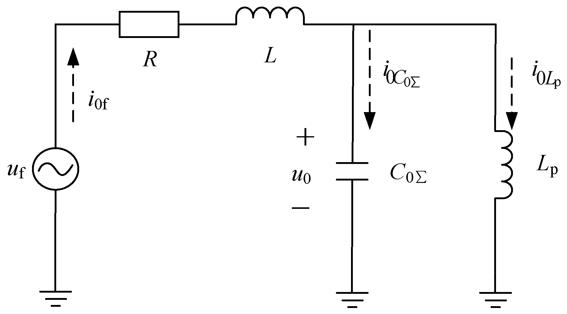
2.1. High-Resistance Grounding Fault Equivalent Circuit

Since the fault transition resistance R_f can reach thousands of ohms or even higher when an HIG fault occurs, the equivalent resistance R can be equivalent to 3R_f, and the equivalent inductance L in Figure 1 can be ignored. Accordingly, the transient process of an HIG fault is only the parallel resonance of C_0∑ and L_p. Therefore, the equivalent circuit can be obtained, as shown in Figure 2.

In the figure, C_0j denotes the zero-sequence capacitance distributed to the ground of a feeder j, and $C_{0\sum }={\displaystyle \sum _{j=1}^n{C}_{0j}}$ where n represents the number of feeders and u_0f is the zero-sequence bus voltage.

The differential equation can be derived according to Figure 2 as follows:

$$\{\begin{array}{l}{u}_{\mathrm{f}}\left(t\right)=R(C_{0\sum }\frac{\mathrm{d}{u}_{0\mathrm{f}}}{\mathrm{d}t}+i_{0L_{\mathrm{p}}})+u_{0\mathrm{f}}\\ u_{0\mathrm{f}}=L_{\mathrm{p}}\frac{\mathrm{d}{i}_{0L_{\mathrm{p}}}}{\mathrm{d}t}\end{array}$$

(1)

The characteristic root obtained as follows:

$$p_{1,2}=-\frac{1}{2R{C}_{0\sum }}\pm \sqrt{{(\frac{1}{2R{C}_{0\sum }})}^2-\frac{1}{L_{\mathrm{p}}{C}_{0\sum }}}$$

(2)

In this study, only the transient calculation of under- and over-damped states is analyzed.

2.2. Transient Calculation of Over-Damped State

Under over-damping conditions, P₁ and P₂ are two real numbers, $P_1\ne P_2$, and

$$R<\frac{1}{2}\sqrt{\frac{L_{\mathrm{p}}}{C_{0\sum }}}=\frac{1}{2}{\omega }_0{L}_{\mathrm{p}}\sqrt{1-v}\approx \frac{1}{2}{\omega }_0{L}_{\mathrm{p}}$$

(3)

where v is the compensation detuning degree of the arc suppression coil, $-0.1\le v\le 0$.

The suppression coil current is calculated by

$$i_{0L_{\mathrm{p}}}=i_{0L_{\mathrm{P}}\_\mathrm{P}}+i_{0L_{\mathrm{P}}\_\mathrm{T}}=B\sin \left({\omega }_{0}t+\phi \right)+A_1{\mathrm{e}}^{p_{1}t}+A_2{\mathrm{e}}^{p_{2}t}$$

(4)

where $i_{0L_{\mathrm{P}\text{\_}}\mathrm{P}}=B\sin ({\omega }_{0}t+\phi )$ denotes the power frequency quantity and $i_{0L_{\mathrm{P}\text{\_}\mathrm{T}}}$ is the transient quantity.

$$\{\begin{array}{l}B=\frac{U_{\mathrm{m}}}{\left|Z\right|}\frac{1}{1-{\omega }_0^2{L}_{\mathrm{P}}{C}_{0\sum }}\\ Z=R+\frac{\mathrm{j}{\omega }_0{L}_{\mathrm{P}}}{1-{\omega }_0^2{L}_{\mathrm{P}}{C}_{0\sum }}\\ A_1=\frac{p_{2}B\sin \phi -{\omega }_{0}B\cos \phi }{p_1-p_2}\\ A_2=\frac{{\omega }_{0}B\cos \phi -p_{1}B\sin \phi }{p_1-p_2}\\ \phi =\theta -\arctan \frac{{\omega }_0{L}_{\mathrm{P}}}{R\left(1-{\omega }_0^2{L}_{\mathrm{P}}{C}_{0\sum }\right)}\end{array}$$

(5)

Therefore, the bus zero-sequence voltage can be obtained as

$$u_{0\mathrm{f}}=u_{0\mathrm{f}\_\mathrm{P}}+u_{0\mathrm{f}\_\mathrm{T}}$$

(6)

where $u_{0\mathrm{f}\_\mathrm{P}}=L_{\mathrm{P}}{\omega }_{0}B\cos \left({\omega }_{0}t+\phi \right)$ is the power frequency, while $u_{0\mathrm{f}\_\mathrm{T}}=L_{\mathrm{P}}\left(p_1{A}_1{\mathrm{e}}^{p_{1}t}+p_2{A}_2{\mathrm{e}}^{p_{2}t}\right)$ denotes the transient process.

The zero-sequence capacitance current of feeder i to the ground can be obtained as

$$i_{C_{0i}}=C_{0i}\frac{\mathrm{d}{u}_{0\mathrm{f}}}{\mathrm{d}t}=-{\omega }_0^2{C}_{0i}{L}_{\mathrm{P}}B\sin \left({\omega }_{0}t+\phi \right)+L_{\mathrm{P}}{p}_1^2{A}_1{C}_{0i}{\mathrm{e}}^{p_{1}t}+L_{\mathrm{P}}{p}_2^2{A}_2{C}_{0i}{\mathrm{e}}^{p_{2}t}$$

(7)

For a healthy feeder, zero-sequence current i_0i and zero-sequence capacitance current $i_{C_{0i}}$ are expressed as

$$\begin{array}{cc}{i}_{0i}=i_{C_{0i}},& i=1,2,\cdots ,n-1\end{array}$$

(8)

The zero-sequence current flowing through the fault point is given by

$$i_{0\mathrm{f}}=i_{0L_{\mathrm{P}}}+i_{0C_{0\sum }}=B\sin \left({\omega }_{0}t+\phi \right)+A_1{\mathrm{e}}^{p_{1}t}+A_2{\mathrm{e}}^{p_{2}t}+L_{\mathrm{P}}{C}_{0\sum }\left[A_1{p}_1^2{\mathrm{e}}^{p_{1}t}+A_2{p}_2^2{\mathrm{e}}^{p_{2}t}-{\omega }_0^{2}B\sin \left({\omega }_{0}t+\phi \right)\right]$$

(9)

From Equations (6), (7) and (9), it can be seen that all transient components are composed of DC components with attenuation, and the attenuation factor is directly related to the transition resistance, which decreases with the increase in the transition resistance. The duration of transient process is hundreds of microseconds to tens of milliseconds.

2.3. Transient Calculation of Under-Damped State

In the under-damped state, a fault is generally exhibited with HIG, and P₁ and P₂ are a pair of complex roots:

$$R>\frac{1}{2}{\omega }_0{L}_{\mathrm{p}}$$

(10)

The arc suppression coil current is given by

$$i_{0L_{\mathrm{p}}}=i_{0L_{\mathrm{P}}\_\mathrm{P}}+i_{0L_{\mathrm{P}}\_\mathrm{T}}$$

(11)

The transient zero-sequence current of the arc suppression coil is obtained as

$$i_{0L_{\mathrm{P}}\_\mathrm{T}}={\mathrm{e}}^{-\delta t}\left[A_3\cos \left({\omega }_{\mathrm{f}}t\right)+A_4\sin \left({\omega }_{\mathrm{f}}t\right)\right]$$

(12)

where δ is the attenuation factor and ω_f is the angular resonance frequency, which are, respectively, given by

$$\delta =\frac{1}{2R{C}_{0\sum }}$$

(13)

$${\omega }_{\mathrm{f}}=\sqrt{\frac{1}{L_{\mathrm{p}}{C}_{0\sum }}-{(\frac{1}{2R{C}_{0\sum }})}^2}=\sqrt{{\omega }_0^2\left(1-v\right)-{\delta }^2}$$

(14)

$$\{\begin{array}{l}{A}_3=-B\sin \phi \\ A_4=\frac{-\delta B\sin \phi -{\omega }_{0}B\cos \phi }{{\omega }_{\mathrm{f}}}\end{array}$$

(15)

Therefore, the bus zero-sequence voltage is calculated by

$$u_{0\mathrm{f}}=u_{0\mathrm{f}\_\mathrm{P}}+u_{0\mathrm{f}\_\mathrm{T}}$$

(16)

where the transient component of the zero-sequence voltage is given by

$$u_{0\mathrm{f}\_\mathrm{T}}=L_{\mathrm{p}}{\mathrm{e}}^{-\delta t}[\left(A_4{\omega }_{\mathrm{f}}-A_3\delta \right)\cos \left({\omega }_{\mathrm{f}}t\right)-\left(A_3{\omega }_{\mathrm{f}}+A_4\delta \right)\sin \left({\omega }_{\mathrm{f}}t\right)]$$

(17)

The capacitance current i_C0i of feeder i to the ground is given by

$$\begin{array}{l}{i}_{C_{0i}}=C_{0i}\frac{\mathrm{d}{u}_{0\mathrm{f}}}{\mathrm{d}t}=-{\omega }_0^2{C}_{0i}{L}_{\mathrm{P}}B\sin \left({\omega }_{0}t+\phi \right)+\\ C_{0i}{L}_{\mathrm{P}}\left({\delta }^2{A}_3-{\omega }_{\mathrm{f}}^2{A}_3-2\delta A_4{\omega }_{\mathrm{f}}\right){\mathrm{e}}^{-\delta t}\cos \left({\omega }_{\mathrm{f}}t\right)+C_{0i}{L}_{\mathrm{P}}\left({\delta }^2{A}_4-{\omega }_{\mathrm{f}}^2{A}_4+2\delta A_3{\omega }_{\mathrm{f}}\right){\mathrm{e}}^{-\delta t}\sin \left({\omega }_{\mathrm{f}}t\right)\end{array}$$

(18)

The zero-sequence current flowing through the fault point is calculated by

$$\begin{array}{l}{i}_{0\mathrm{f}}=i_{0L_{\mathrm{P}}}+i_{0C_{0\sum }}=\left(1-{\omega }_0^2{C}_{0\sum }{L}_{\mathrm{P}}\right)B\sin \left({\omega }_{0}t+\phi \right)+\left[A_3+C_{0\sum }{L}_{\mathrm{P}}\left({\delta }^2{A}_3-{\omega }_{\mathrm{f}}^2{A}_3-2\delta A_4{\omega }_{\mathrm{f}}\right)\right]{\mathrm{e}}^{-\delta t}\cos \left({\omega }_{\mathrm{f}}t\right)+\\ \left[A_4+C_{0\sum }{L}_{\mathrm{P}}\left({\delta }^2{A}_4-{\omega }_{\mathrm{f}}^2{A}_4+2\delta A_3{\omega }_{\mathrm{f}}\right)\right]{\mathrm{e}}^{-\delta t}\sin \left({\omega }_{\mathrm{f}}t\right)\end{array}$$

(19)

From the above analysis, it can be seen that the transient process is an attenuated oscillation, and the attenuation factor is inversely proportional to the transition resistance. According to Equation (14), the resonant frequency increases with the increase in the transition resistance. The resonant frequency has a maximum value:

$${\omega }_{\mathrm{f}.\max }={\omega }_0\sqrt{\left(1-v\right)}\approx 326\mathrm{rad}/\mathrm{s}$$

(20)

At this time, the corresponding frequency is about 52 Hz. For a certain system, with the increase in resistance, the resonant frequency monotonically increases from zero and the maximum frequency is slightly larger than the operating frequency.

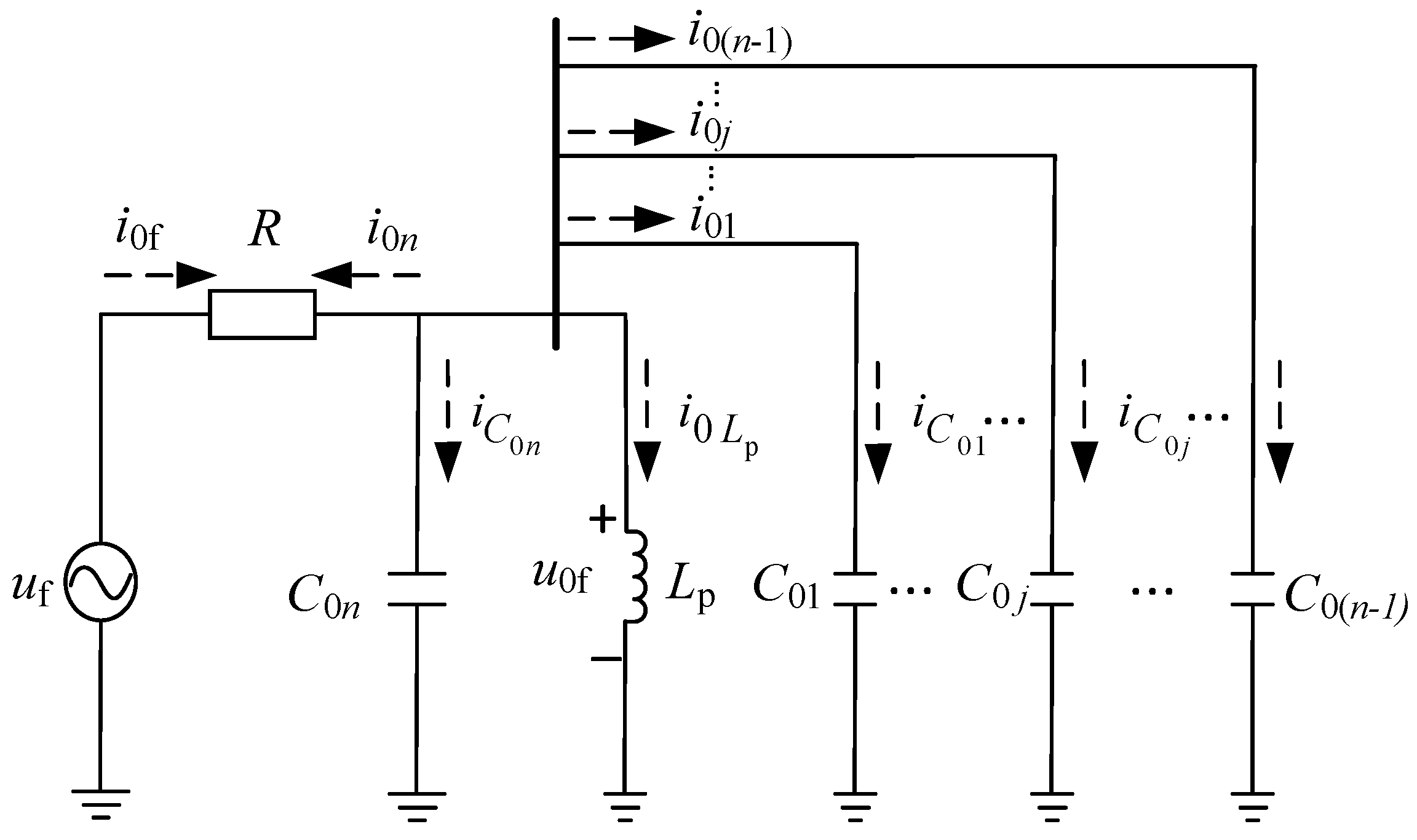
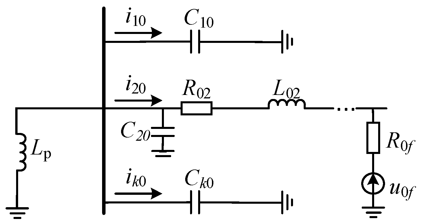
2.4. Analysis of Zero-Sequence Impedance Characteristics of High-Resistance Grounding

For a distribution network under normal conditions, the input impedance of a feeder is given by

$$Z_{oc}\left(\omega \right)=\frac{\dot{U}}{\dot{I}}=Z_c\coth \left(\gamma l\right)$$

(21)

where $Z_c=\sqrt{\left(R_l+\mathrm{j}\omega L_l\right)/\mathrm{j}\omega C_l}$ is the characteristic impedance of a line; $\gamma =\sqrt{\mathrm{j}\omega R_l{C}_l-{\omega }^2{L}_l{C}_l}$ is the propagation coefficient; l is the length of the feeder; and R_l, L_l, and C_l denote the resistance, inductance, and distributed capacitance per unit length of the line, respectively.

Since the transition resistance in the case of an HIG fault is relatively large, the line resistance is ignored in the equivalent circuit shown in Figure 2. By simplifying Equation (20), the zero-sequence impedance at the input end of a feeder k can be obtained by substituting ω = 2πf:

$$Z_{\mathrm{oc}k}\left(f\right)=\frac{{\dot{U}}_0}{{\dot{I}}_{0k}}=\sqrt{\frac{L_{0k}}{C_{0k}}}\coth \left(l_k\sqrt{-4{\mathsf{\pi }}^2{f}^2{L}_{0k}{C}_{0k}}\right)=-\mathrm{j}\sqrt{\frac{L_{0k}}{C_{0k}}}\cot \left(2\mathsf{\pi }f\sqrt{L_k{C}_k}\right)$$

(22)

where L_0k is the zero-sequence inductance of feeder k, L_k = L_0kl_k, C_0k is the zero-order distributed capacitance, and C_k = C_0kl_k.

2.4.1. The Zero-Sequence Impedance Characteristics of the Normal Feeder

In Equation (22), once $2\mathsf{\pi }f\sqrt{L_{\mathrm{k}}{C}_{\mathrm{k}}}=\mathsf{\pi }/2$, then $Z_{\mathrm{oc}k}\left(f\right)=0$; that is, $f=f_{\mathrm{k}}=1/4\sqrt{L_{\mathrm{k}}{C}_{\mathrm{k}}}$, where feeder k resonates for the first time. Given $0\le f<f_{\mathrm{k}}$, the zero-sequence impedance of feeder k is capacitive. With the increase in the frequency, the zero-sequence impedance of feeder k will no longer be uniform. Therefore, when the line’s impedance characteristics are used for line selection, the frequency band higher than f_k will not be suitable for the fault line selection. Define f_min is as the minimum resonant frequency of feeder k:

$$f_{\min }=\min \left(\frac{1}{4\sqrt{L_{\mathrm{k}}{C}_{\mathrm{k}}}}\right)$$

(23)

According to the line parameters in Figure 2, the minimum resonance frequency f_min is very high, generally several thousand of hertz or even tens of thousands of hertz, so the zero-sequence impedance characteristics of the healthy lines at a certain sampling frequency are capacitive.

2.4.2. Zero-Sequence Impedance Characteristics of Faulty Feeder

Assuming that a single-phase ground fault occurs at feeder 2 in Figure 2, a healthy feeder can be equalized to a lumped parameter capacitor, whereas the equivalent impedance of a faulty feeder represents the resulting impedance of all healthy lines and arc suppression coils, which is the parallel impedance of a feeder’s equivalent lumped-parameter capacitor and an inductor. The simplified zero-sequence network is shown in Figure 3, where C_k0 is the equivalent lumped parameter capacitance of a healthy feeder k.

If the arc suppression coil is considered to be ideal, the zero-sequence equivalent admittance Y_2(f) of faulty feeder 2 is obtained as follows:

$$Y_2\left(f\right)=\frac{1}{Z_2\left(f\right)}=\frac{{\dot{I}}_{02}}{{\dot{U}}_0}=-\frac{{\dot{I}}_{L_p}+{\displaystyle \sum _{k=1,k\ne 2}^m{\dot{I}}_{k0}}}{{\dot{U}}_0}=-\frac{1}{\mathrm{j}2\mathsf{\pi }f{L}_p}-\mathrm{j}2\mathsf{\pi }f{\displaystyle \sum _{k=1,k\ne 2}^m{C}_k{}_0}$$

(24)

Once the frequency f gradually increases from 0, the zero-sequence impedance of the feeder will change from inductive to capacitive. According to Equation (20), the resonant frequency also has an upper limit, so f_res is much smaller than f_min. Based on that, after an SPG fault occurs, the faulty feeder becomes inductive in the frequency range (0, f_res), whereas in the frequency range of (f_res, f_min), the faulty feeder is capacitive. Therefore, in this study, the frequency band (0, f_res) is defined as a low-frequency band, while the frequency band (f_res, f_min) is defined as a high-frequency band.

3. Fault Detection Algorithm

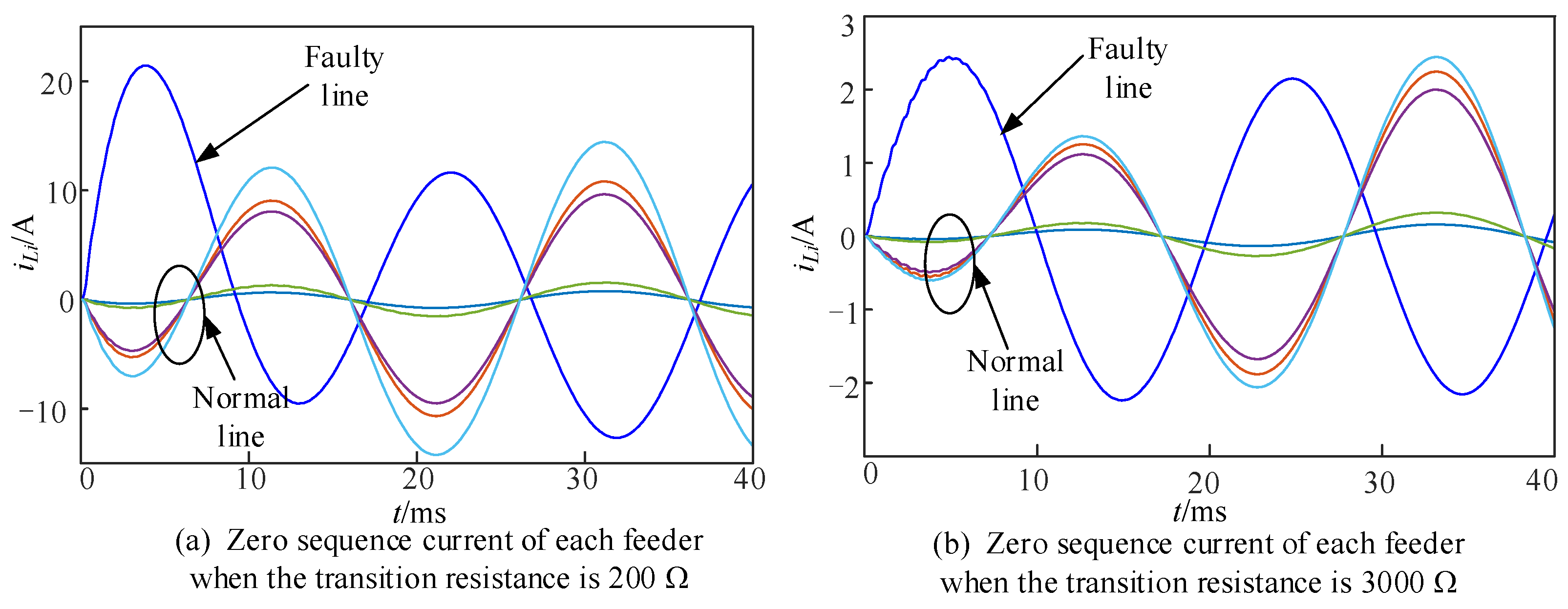
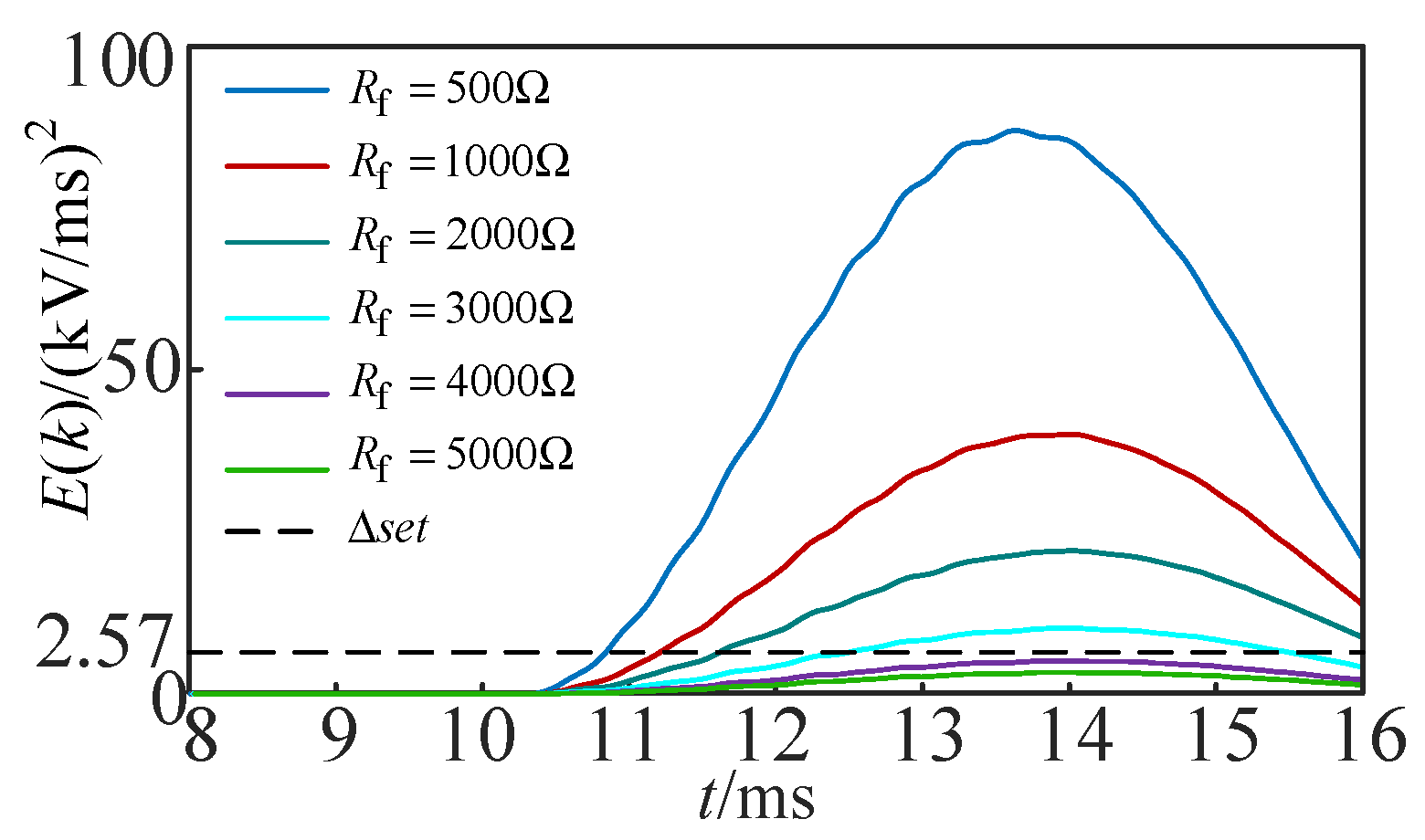
3.1. Comparison of Fault Signals under Different Transition Resistances

In the simulation model shown in Figure 4, assuming that an SPG fault occurs on feeder L1 and 10 km away from the bus with a transition resistance of 200 Ω and 3000 Ω, the comparison of the zero-sequence current amplitude of each feeder is shown in Figure 5.

It can be seen that when an SPG fault with a transition resistance of 3000 Ω occurs, the zero-sequence current amplitude of each feeder obviously decreases. With the increase in transition resistance, the fault electrical quantity will continuously decrease, and the detection difficulty of the HRG fault will increase accordingly.

Taking into account the decomposition of any three-phase system into zero-sequence impedance, positive sequence impedance, and negative sequence impedance, this study focuses on zero-sequence impedance as the primary fault feature. Voltage drops, although it can result from momentary closings, are not considered a fault feature, due to the potential for misjudgment. The zero-sequence appearance arises from the analysis of three-phase asymmetric components being decomposed into symmetrical components (positive and negative sequence) and zero-sequence components in the same direction when there is voltage and current asymmetry in the system. By utilizing the phase sequence component and zero-sequence component method, a three-phase equivalent circuit model is derived based on zero-sequence grounding impedance. This equivalent circuit is then applied to calculate the three-phase short-circuit current interruption process for effectively grounded neutral systems and ungrounded neutral systems.

3.2. High-Resistance Ground Fault Detection Algorithm

The conventional fault line selection device operates by evaluating if the neutral point voltage exceeds the preset value of 0.15U_m within the power frequency band, determining the occurrence of a fault. However, in situations where the system is grounded with high resistance, the zero-sequence voltage may be lower than 15% of the phase voltage, resulting in the failure of the line selection device. To address this issue, a new approach utilizes the variation in the zero-sequence voltage to determine whether an SPG fault exists in the system. Since the three-phase parameters of an RGDN are not perfectly symmetrical, the zero-sequence voltage remains relatively small under normal system operating conditions but experiences a substantial increase after a fault occurs. Hence, the zero-sequence voltage serves as an ideal initial indicator for detecting high-resistance grounding faults.

To eliminate the influence of the three-phase asymmetry of the RGDN and abnormal fluctuations in the zero-sequence voltage in the actual operation, the zero-sequence voltage change between two adjacent periods is used as an initial indicator of the grounding line selection to avoid the misjudgment caused by zero-sequence voltage fluctuations in normal system operation. The zero-sequence voltage gradient sum c_dif(k) is obtained as follows:

$$c_{\mathrm{dif}}\left(k\right)=\left[u_0\left(k\right)-u_0\left(k-1\right)\right]/\mathsf{\Delta }t$$

(25)

E(k) is the zero-order voltage gradient sum, as shown in Formula (26):

$$E\left(k\right)={\displaystyle \sum _{n=k-K+1}^k{\left[c_{\mathrm{dif}}\left(n\right)\right]}^2}$$

(26)

where k represents the current sampling point, Δt represents the sampling interval in ms, K represents the number of sampling points in a certain time window, and k ≥ K.

The zero-sequence voltage gradient sum can be set as the starting threshold according to the setting value of the traditional line selection device. The setting value is generally 15% of the rated phase voltage amplitude, namely, the amplitude is 1.22 kV, as shown in Figure 6a. When the number of sampling points K in a certain time window is three, four, five, or six, the threshold Δset of E(k) is 1.54, 2.05, 2.57, or 3.08 (kV/ms)², respectively, as shown in Figure 6b.

To evaluate the pros and cons of the two fault detection methods, different fault types were set in the simulation model of an RGDN in Figure 4, and the start-up times of the two methods were compared and analyzed. It was assumed that extreme faults with a small fault closing angle and different transition resistances would occur at the end of line L₃. The operation procedure of the fault detection method, which starts by detecting whether the neutral point voltage exceeds the preset voltage value (15%U_m), is shown in Figure 7. The single-phase ground fault with a small angle of R_f = 3000 Ω occurred at the end of line L₃, and the value of K was taken as five. The zero-sequence voltage abrupt change was used as a starting result, as shown in Figure 8. The starting result of using the zero-sequence voltage gradient sum under different transition resistances at K = 5 is presented in Figure 9.

As shown in Figure 7, when a small-angle high-resistance grounding fault occurred at the end of the line, the transition resistance of 4000 Ω could be identified using the traditional fault detection method, and the fault detection time will be longer with the increase in the transition resistance. Once the transition resistance exceeds 5000 Ω, the traditional fault detection method becomes unable to work satisfactorily.

In Figure 8, E(1) = 0.86 (kV/ms)², E(2) = 2.70(kV/ms)², and E(3) = 7.09(kV/ms)². When the abrupt change in the zero-sequence voltage was used as a starting moment, the gradient sum of the zero-sequence voltage increased sharply. When K = 5 and R_f = 3000 Ω, the starting time was only 2 ms, and the line selection device had a short starting time and fast speed. As shown in Figure 9, when the zero-sequence voltage gradient sum was used as a fault starting method, the starting time was much shorter than that of the traditional starting method, and the starting sensitivity was related to the value of K within a certain time window. Therefore, by selecting an appropriate value for K according to the actual operation of a distribution network, the sensitivity of the starting method could be improved, and the problem of impossible operation of the protection device during high-resistance grounding could be solved. The comparison of the starting time between using the zero-sequence voltage abrupt change as a starting indicator and the traditional neutral point voltage detection method is shown in

Table 1. Comparison of startup time.

	Starting System	15%Um	Zero-Sequence Voltage Gradient Sum
Rf/Ω			K = 3	K = 4	K = 5	K = 6
Start time (ms)	500	12.8	10.7	10.8	10.8	10.9
	1000	12.9	10.9	11.0	11.1	11.2
	2000	13.5	11.3	11.4	11.4	11.5
	3000	13.9	12.0	12.1	12.1	12.2
Interval time (ms)	500	2.8	0.7	0.8	0.8	0.9
	1000	2.9	0.9	1.0	1.1	1.2
	2000	3.5	1.3	1.4	1.4	1.5
	3000	3.9	2.0	2.1	2.1	2.2

, and the fault occurrence time was 10.0 ms.

Compared to the results in Table 1, when the transition resistance is set between 500 and 3000 Ω, the starting method of using the zero-sequence voltage abrupt change can greatly improve the initial time of the line selection device. The initial time of the traditional starting method for detecting whether the neutral point voltage exceeds the preset value is generally between 2 ms and 4 ms, whereas the initial time when using the zero-sequence voltage abrupt change as the starting parameter is between 0.5 ms and 2 ms. This result indicates that using the zero-sequence voltage abrupt change as the starting parameter can greatly improve the initial time of the line selection device, quickly respond to ground fault, and meet the requirements of an intelligent distribution network.

Based on the above analysis, when the traditional fault detection method is used, it can effectively identify the HIG fault up to 4000 Ω. Meanwhile, when the zero-sequence voltage mutation is used, the HIG fault can be effectively identified only up to 3000 Ω, but the initial time is much shorter than that of the traditional fault detection method. Therefore, the combination of the zero-sequence voltage mutation and traditional phase voltage of 15% is selected to be used as a detection method of an SPG fault in a distribution network, which improves the speed of a line selection device.

4. Principle for Fault Line Selection

The correlation coefficient is used to explain the correlation between two waveforms. The correlation coefficient is determined through human expert experience in four different levels as given in (27). Similar classification of the levels can also be found in [37,38].

$$\rho =\frac{{\displaystyle \sum _{n=0}^{N-1}x\left(n\right)y\left(n\right)}}{\sqrt{{\displaystyle \sum _{n=0}^{N-1}{x}^2\left(n\right)}{\displaystyle \sum _{n=0}^{N-1}{y}^2\left(n\right)}}},\{\begin{array}{c}\left|\rho \right|<0.3\begin{array}{c}\end{array}\\ 0.3\le \left|\rho \right|<0.5\\ 0.5\le \left|\rho \right|<0.8\\ 0.8\le \left|\rho \right|<1\end{array}\begin{array}{c}\mathrm{No}\mathrm{correlation}\\ \mathrm{Low}\mathrm{correlation}\\ \mathrm{Moderate}\mathrm{correlation}\\ \mathrm{High}\mathrm{correlation}\end{array}$$

(27)

4.1. Correlation Coefficient of Impedance Characteristics of Normal Feeder

Assume ${\rho }_h$ and ${\rho }_l$ are the high- and low-frequency band correlation coefficients of the voltage and current, which are given by Equation (28), respectively. In Equation (28), u_0l(n) and i_0l(n) denote the low-frequency components of the voltage and current, respectively, while u_0h(n) and i_0h(n) are their corresponding high-frequency components.

$${\rho }_h=\frac{{\displaystyle \sum _{n=0}^N\frac{\mathrm{d}{u}_{0h}\left(n\right)}{\mathrm{d}t}{i}_{0h}\left(n\right)}}{\sqrt{{\displaystyle \sum _{n=0}^N{\left(\frac{\mathrm{d}{u}_{0h}\left(n\right)}{\mathrm{d}t}\right)}^2}{\displaystyle \sum _{n=0}^N{i}_{0h}{}^2\left(n\right)}}},{\rho }_l=\frac{{\displaystyle \sum _{n=0}^N\frac{\mathrm{d}{u}_{0l}\left(n\right)}{\mathrm{d}t}{i}_{0l}\left(n\right)}}{\sqrt{{\displaystyle \sum _{n=0}^N{\left(\frac{\mathrm{d}{u}_{0l}\left(n\right)}{\mathrm{d}t}\right)}^2}{\displaystyle \sum _{n=0}^N{i}_{0l}{}^2\left(n\right)}}}$$

(28)

According to the above analysis, the impedance characteristics of the healthy feeder in the whole sampling frequency band are capacitive, so the current of the healthy feeder in this frequency band is proportional to the voltage derivative. The coefficients ${\rho }_h$ and ${\rho }_l$ of healthy feeders should be highly correlated, and their correlation coefficient $\left|\rho \right|$ should be greater than 0.8.

4.2. Correlation Coefficient of Impedance Characteristics of Faulty Feeder

The impedance characteristics of fault lines are inductive in the low-frequency band but capacitive in the high-frequency band. In the high-frequency band, sudden change directions of the zero-sequence currents of the faulty and healthy feeders are opposite, and the current amplitude of the faulty feeder is equal to the sum of the zero-sequence current amplitudes of all healthy lines, which reflects Kirchhoff’s Current Law. Therefore, ${\rho }_h$ of a fault line can be calculated as ${\rho }_h=-1$.

According to the above analysis, the essence of an SPG fault is the parallel resonance of a system. The current flowing through the arc suppression coil is given by Equation (4), where φ denotes the initial phase angle of a fault, and the fault current in the transient process is mainly the power frequency component and the attenuated DC component in the low-frequency band. When φ = 0°, the attenuated DC component reaches the maximum, and when φ = 90°, the attenuated DC component is almost zero. The zero-sequence voltage of a bus has only the power frequency component in the low-frequency band.

The zero-sequence current and bus zero-sequence voltage in two power frequency cycles after a fault occurred were extracted, and the relationship between the two waveforms in the low-frequency band was analyzed. The results were as follows.

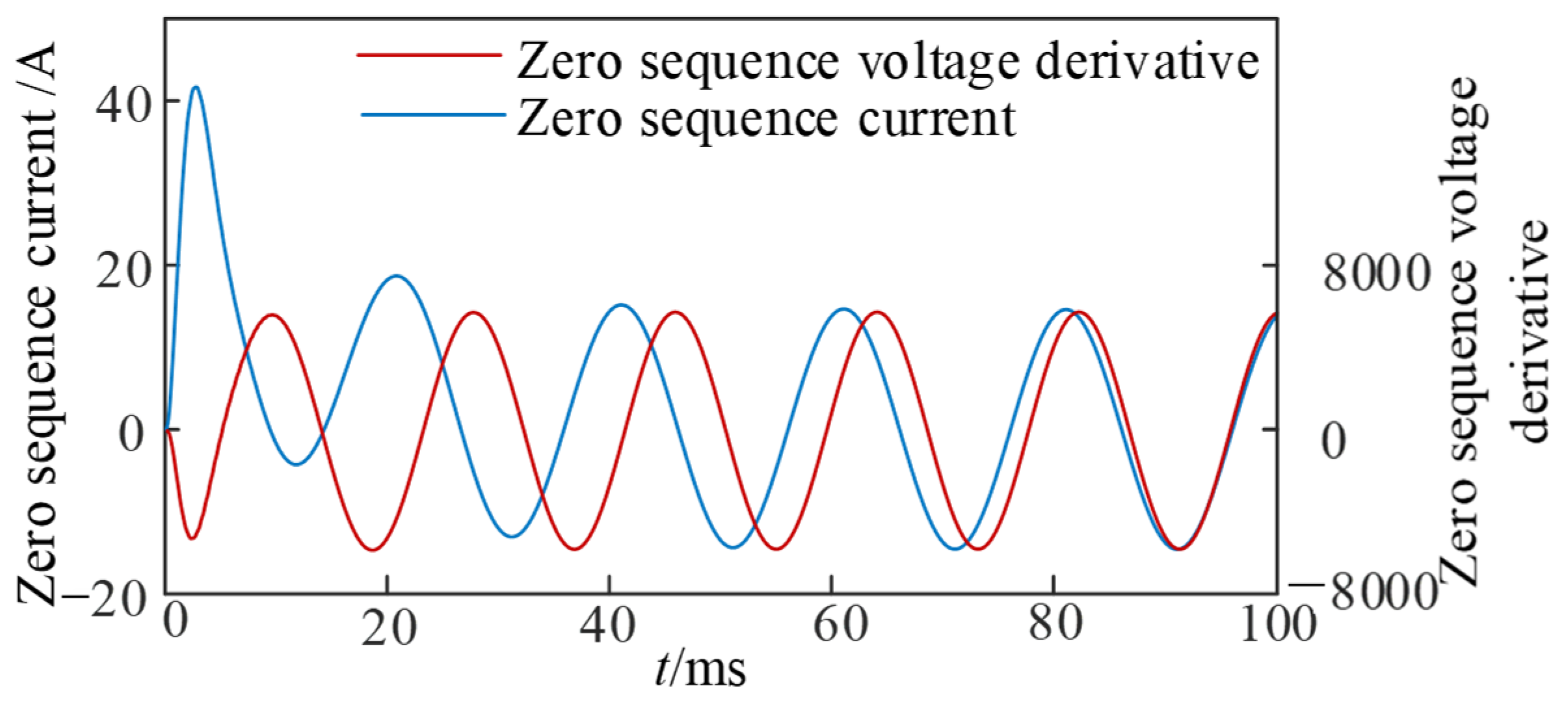
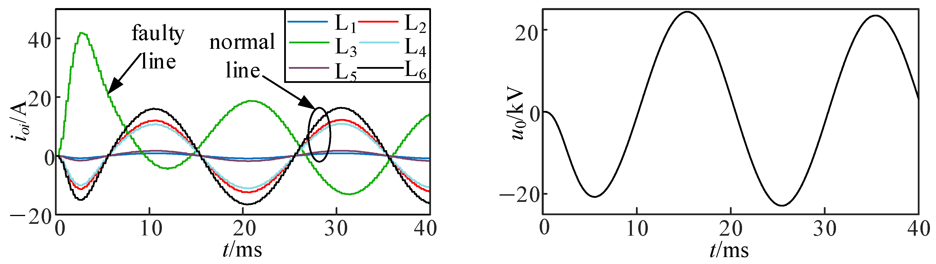
• The waveforms of the current and voltage derivatives at φ = 0° are shown in Figure 10. When the initial phase angle of the fault was one, the attenuation DC component reached the maximum. As shown in Figure 10, the zero-sequence voltage derivative and zero-sequence current waveform of the fault line bus were different in the first two power frequency bands.

In the low-frequency band (φ = 0°), the current and voltage waveforms met the principle of opposite polarity of the first-half wave, so the derivative waveforms of the zero-sequence current and bus zero-sequence voltage was different. In addition, since the attenuation DC component was largest at φ = 0°, and the attenuation period of the fault current was long, only the fault data of two power frequency periods after the fault occurred were extracted and used in the analysis; the correlation between the two waveforms in the low-frequency band was very small, close to zero, when φ = 0°.

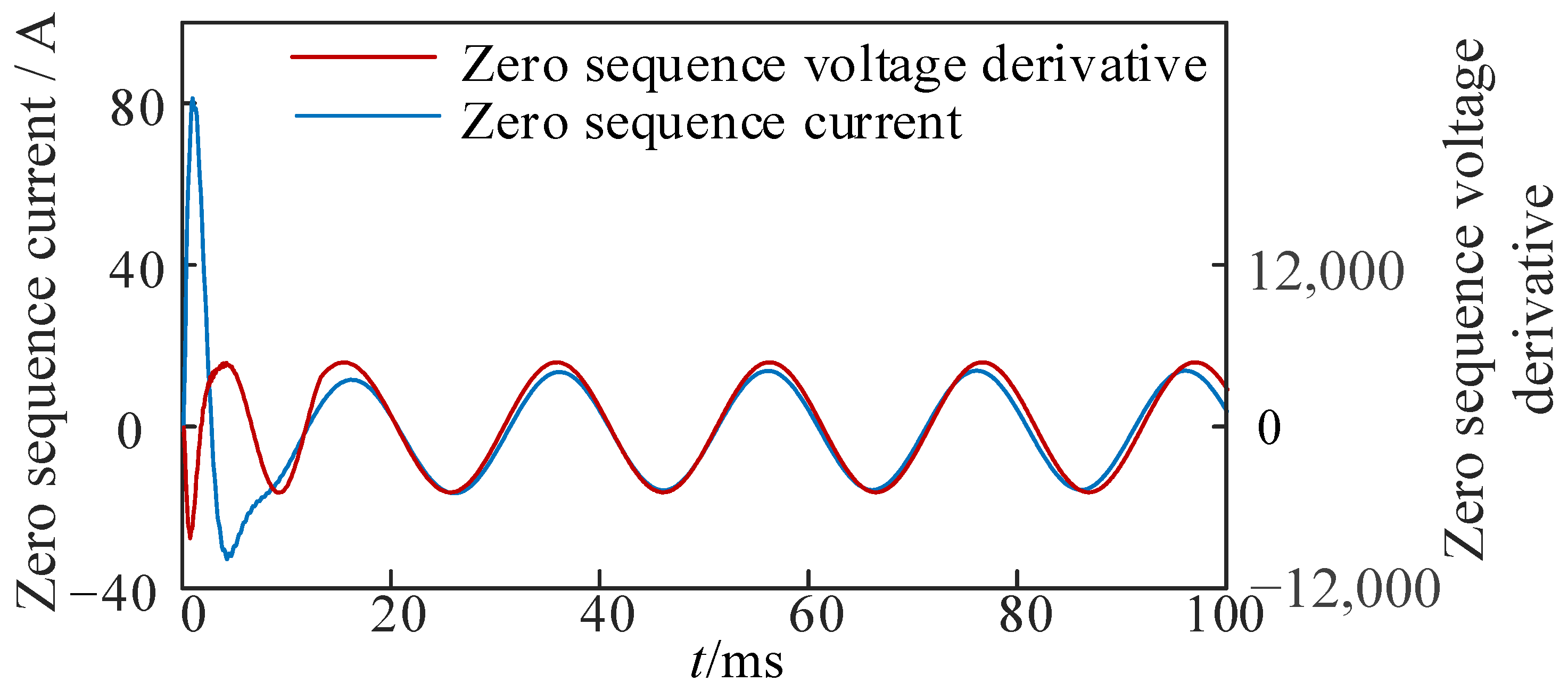
• The waveform of the current and voltage derivatives at φ = 90° are shown in Figure 11. In this case, the attenuation DC component was zero, and the current and voltage waveforms met only the first half-wave principle, as well as the derivatives of the zero-sequence current and bus zero-sequence voltage. Since there was no attenuation component, the polarity of the two waveforms rapidly became the same after the first half-wave.

When φ = 90°, the correlation coefficient between the current and voltage derivative waveforms reached the maximum. The correlation coefficient was between moderate and high, i.e., it was between 0.5 and 1. Consequently, the correlation coefficient ${\rho }_l$ of a fault line in the low-frequency band is given by

$$\{\begin{array}{ll}\theta =0^{\circ },& 0<{\rho }_l<0.3\\ 0^{\circ }<\theta <{90}^{\circ },& 0<{\rho }_l<1\\ \theta ={90}^{\circ },& 0.5<{\rho }_l<1\end{array}$$

(29)

4.3. Line Selection Criterion

The reciprocal correlation coefficient P_k is defined as

$$P_k=\frac{1}{{\rho }_l}-\frac{1}{{\rho }_h}$$

(30)

Based on the previous analysis, ${\rho }_h$ and ${\rho }_l$ of healthy lines should be highly correlated, and the reciprocal correlation coefficient of the healthy lines is a value close to zero. According to Equation (30), the correlation coefficient of a fault line in the low-frequency band is one at most, i.e., the reciprocal correlation coefficient of the fault line is a value greater than two. According to the simulation results, the threshold value of the correlation coefficient of the inversion is set to P_set = 0.8. The fault line discrimination matrix is defined as

$$s=\{\begin{array}{l}1\\ -1\end{array}\begin{array}{c},\\ ,\end{array}\begin{array}{c}{P}_{\mathrm{set}}<0.8\\ P_{\mathrm{set}}>0.8\end{array}$$

(31)

The line corresponding to the element “−1” in matrix $s$ is a faulty feeder. If a fault is determined according to the above fault starting criterion, and all the elements in matrix S are “1”, then the fault is determined as a bus fault.

4.4. Fault Line Selection Algorithm

Firstly, the zero-sequence voltage gradient sum and 15% of the rated phase voltage amplitude are used as the fault starting criteria to judge whether the line fails. The specific steps of the fault line selection method are as follows:

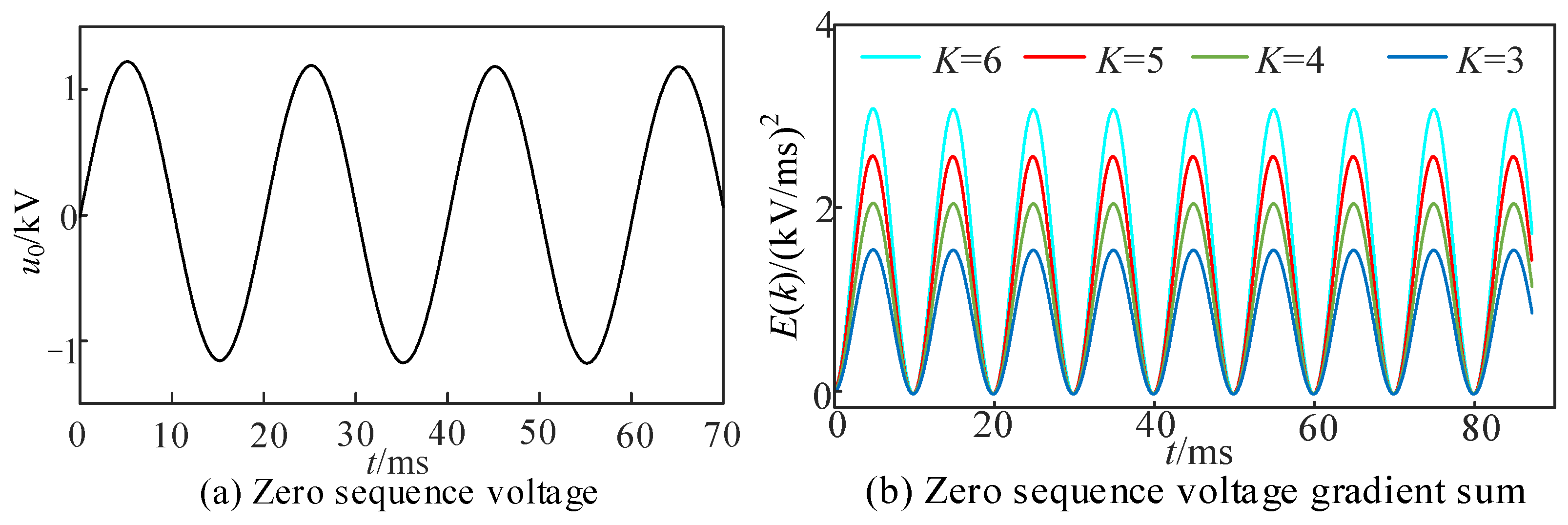
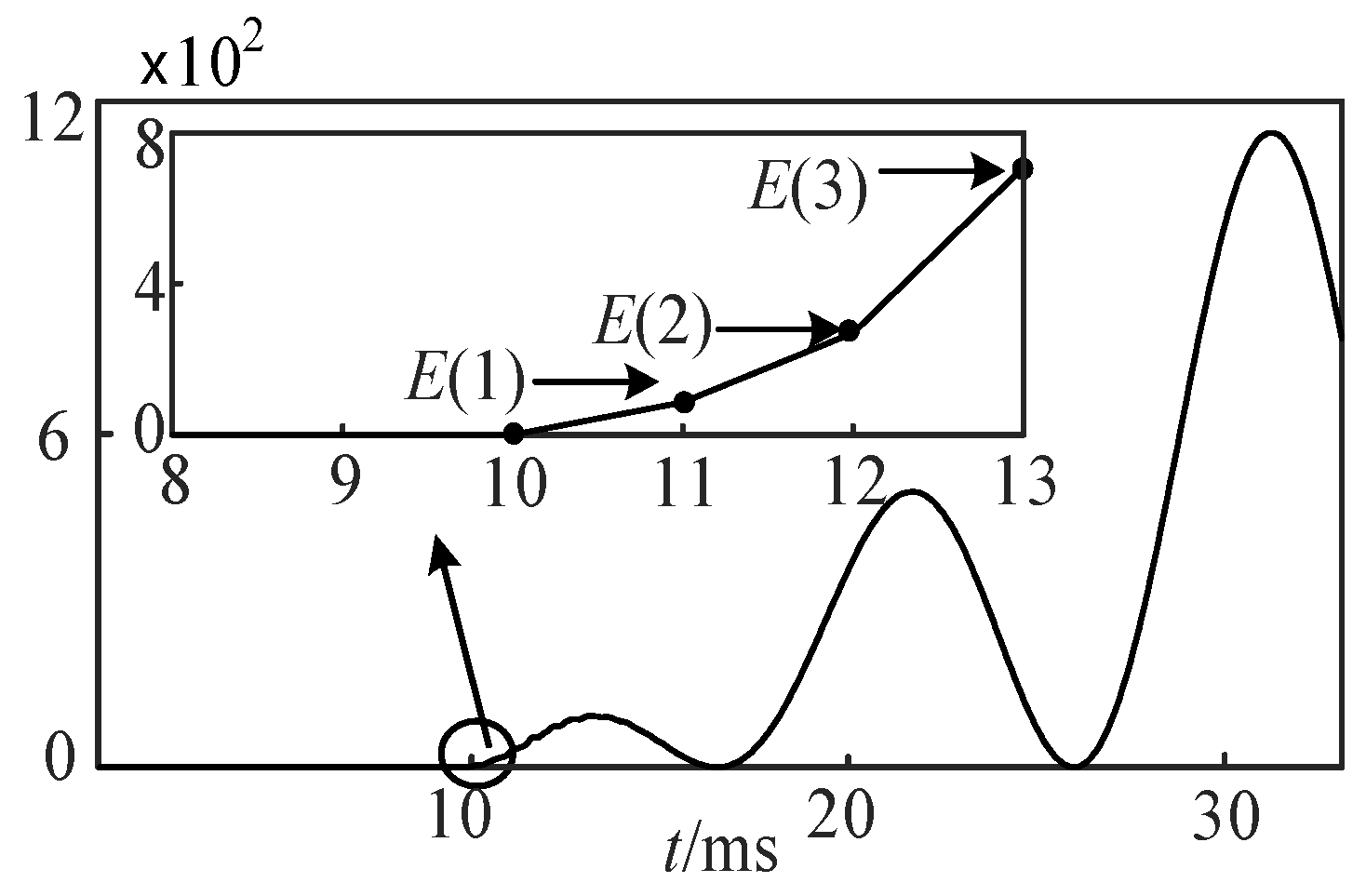
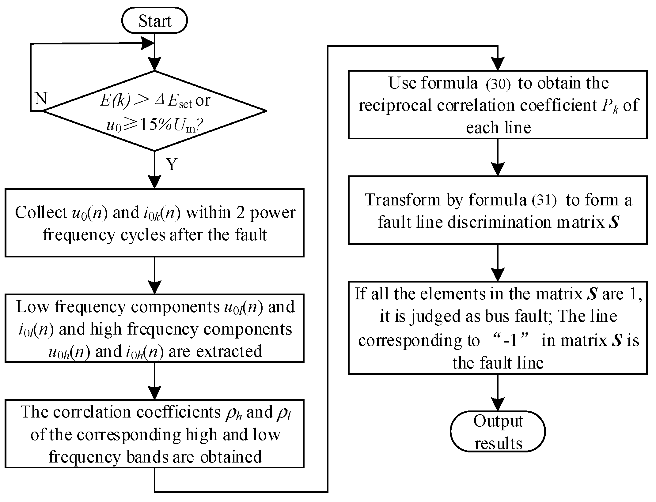
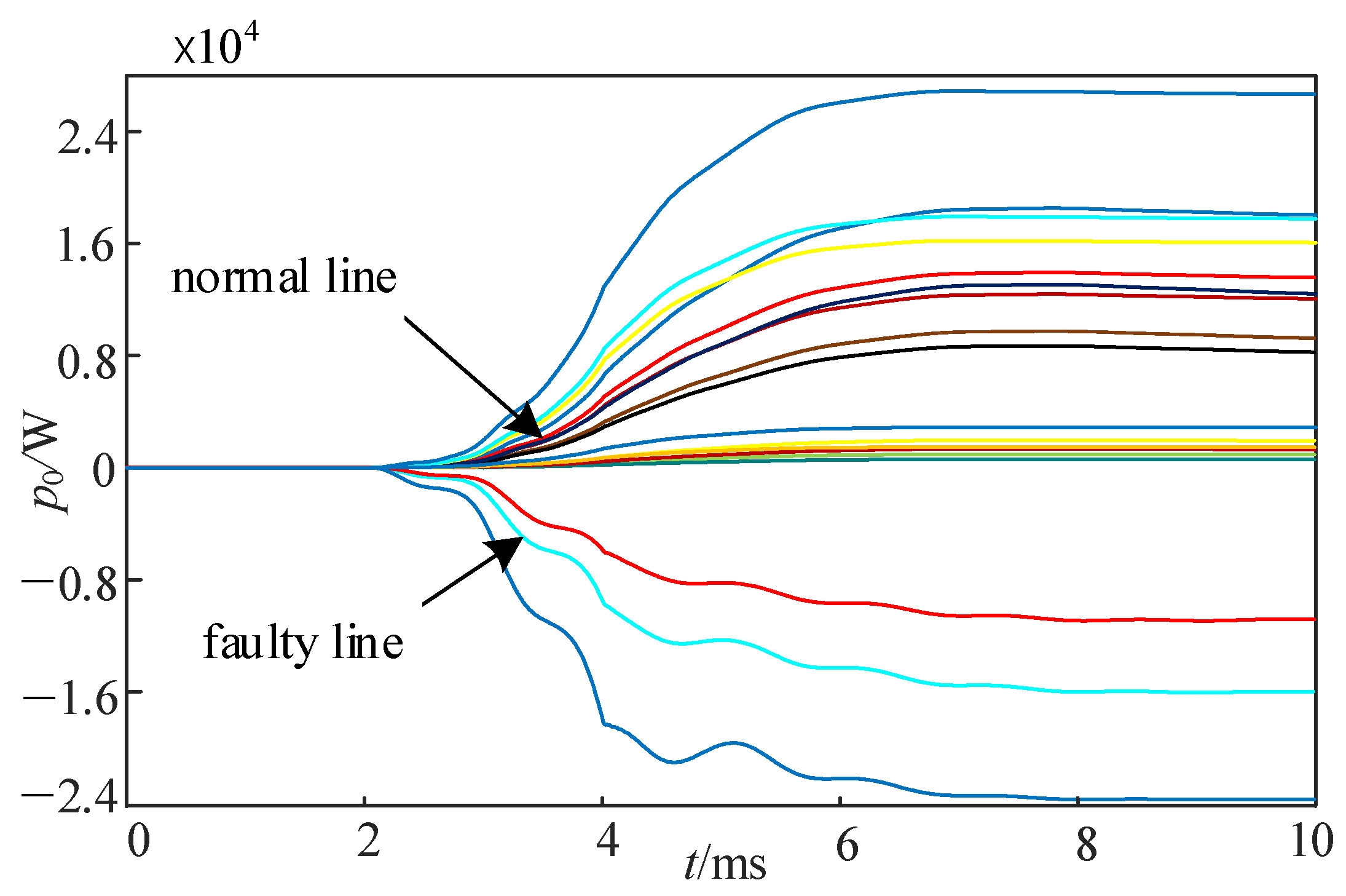
• According to the fault starting criterion, if E(k) > ΔEset or u₀ ≥ 15%U_m, the system is judged to have a fault, and the system collects the line’s zero-sequence current i_0k(n) and the bus zero-sequence voltage u₀(n) of two power frequency cycles.
• The low-frequency components u_0l(n) and i_0l(n) and high-frequency components u_0h(n) and i_0h(n) of the voltage and current are obtained through filtering.
• The data of the high- and low-frequency components of the voltage and current after the fault are extracted for the correlation analysis, and the correlation coefficients ρ_h and ρ_l corresponding to the high- and low-frequency bands, respectively, are obtained.
• The reciprocal correlation coefficient P_k of each line is calculated using Equation (30) and then transformed according to Equation (31) to obtain a fault line discrimination matrix $s$, in which element “−1” indicates a faulty feeder and element “1” indicates a bus fault. The fault line selection process is shown in Figure 12.

5. Simulation Verification

The simulation model of a 10 kV RGDN was built using MATLAB 2019 software, as shown in Figure 4. The system consisted of six feeders and three types of line models. The line parameters are given in

Table 2. Line parameters of the model given in Figure 4.

Line Type	R1/(Ω·km−1)	L1/(mH·km−1)	C1/(μF·km−1)
Overhead line	0.17	1.2100	0.00969
Cable line	0.27	0.2548	0.33910
Line type	R0/(Ω·km−1)	L0/(mH·km−1)	C0/(μF·km−1)
Overhead line	0.23	5.4780	0.0800
Cable line	2.70	1.0191	0.28000

. All loads were set as constant-power loads, transformer T was the main transformer with a transformation ratio of 110 kV/10 kV, and the compensation mode of the arc suppression coil was overcompensation with a compensation coefficient of 10%.

In this study, low-frequency components u_0l(n) and i_0l(n) and high-frequency components u_0h(n) and i_0h(n) of the voltage and current, respectively, were extracted through filtering. The low-frequency range was 0–60 Hz and the high-frequency range was 100–1000 Hz. In the case of a system failure, according to the above-mentioned fault starting algorithm, the zero-sequence voltage change gradient sum or 15% of the rated phase voltage amplitude was higher than the preset threshold; the fault sampling device started working and collected fault data, and the zero-sequence current of each feeder and the zero-sequence voltage of the bus after failure were determined, as shown in Figure 13.

As shown in Figure 13, the zero-sequence current of the faulty feeder is opposite to that of the sound feeder, and the amplitude of the zero-sequence current of the faulty feeder is larger than that of the sound feeder. The filter is used to extract the high- and low-frequency components of zero-sequence current and zero-sequence voltage, which provides the basis for fault line selection.

5.1. Line Selection Method Adaptability Analysis

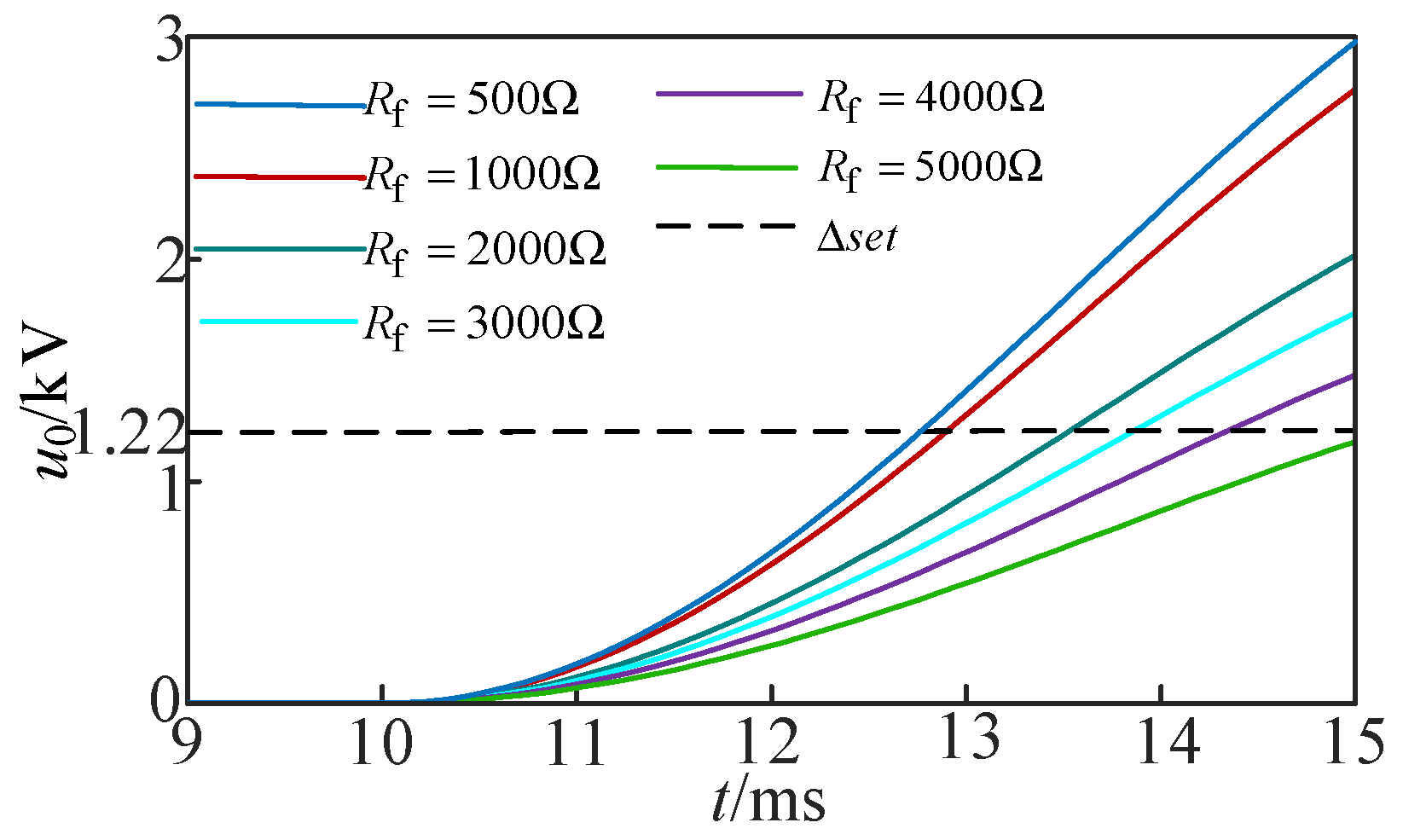
5.1.1. Transition Resistance

With different transition resistances and other faults with the same fault conditions, it was assumed that a single-phase ground fault with an initial phase angle of 30 occurred at a distance of 10 km from the bus at line L₁. The simulation results are shown in

Table 3. Line selection results under different transition resistances.

Rf/Ω	Inversion Correlation Coefficient Pk/P1, P2, P3, P4, P5, P6	Fault Line Discrimination Matrix s	Line Selection Result
200	3.6654, −0.0214, −0.0175, −0.0231, −0.0109, −0.0198	s = [−1 1 1 1 1 1]	Correct
500	3.8374, −0.0213, −0.0212, 0.0235, −0.0330, −0.0250	s = [−1 1 1 1 1 1]	Correct
700	3.4823, 0.0066, −0.0113, −0.0181, −0.0065, −0.0201	s = [−1 1 1 1 1 1]	Correct
1000	3.3891, −0.0227, −0.0355, −0.0247, 0.0032, −0.0402	s = [−1 1 1 1 1 1]	Correct
1500	3.3070, −0.0247, −0.0283, −0.0306, −0.0213,−0.0286	s = [−1 1 1 1 1 1]	Correct
2000	3.2201, −0.0173, −0.0381, −0.0302, 0.0047, −0.0221	s = [−1 1 1 1 1 1]	Correct
3000	3.0504, −0.0287, −0.0293, −0.0178, −0.0145, −0.0198	s = [−1 1 1 1 1 1]	Correct

, where it can be seen that the proposed line selection method could accurately select the fault line with high sensitivity when the fault transition resistance was in the range of 200–3000 Ω.

5.1.2. Fault Closing Angle

It was assumed that in line L1, a single-phase ground fault with a distance of 10 km from the bus and a transition resistance of 1000 Ω occurred. During the analysis, different fault closing angles and different fault phases were used, while the other fault conditions were unchanged. The line selection results are shown in

Table 4. Line selection results under different transition closing angles.

φ/(°)	Fault Phase Separation	Inversion Correlation Coefficient Pk/P1, P2, P3, P4, P5, P6	Fault Line Discrimination Matrix s	Line Selection Result
0	Phase A	9.2850, −0.0277, −0.0116, 0.0077, −0.0144, −0.0115	s = [−1 1 1 1 1 1]	Correct
15	Phase B	3.5714, 0.0027, −0.0219, −0.0130, −0.5146, −0.0073	s = [−1 1 1 1 1 1]	Correct
30	Phase A	3.5006, −0.0211, −0.0139, −0.0043, −0.0103, −0.0415	s = [−1 1 1 1 1 1]	Correct
45	Phase A	3.3607, −0.0058, −0.0180, −0.0153, −0.0158, −0.0096	s = [−1 1 1 1 1 1]	Correct
75	Phase B	3.1436, −0.0433, −0.0253, −0.0210, 0.0042, −0.0244	s = [−1 1 1 1 1 1]	Correct
90	Phase A	2.2661, −0.0130, −0.5146, −0.0439, −0.0243, −0.0247	s = [−1 1 1 1 1 1]	Correct

, where it can be seen that under all fault closing angles and fault phases, the proposed line selection method could accurately select fault lines, indicating that it was not affected by fault closing angles and fault phases and had high sensitivity and strong reliability.

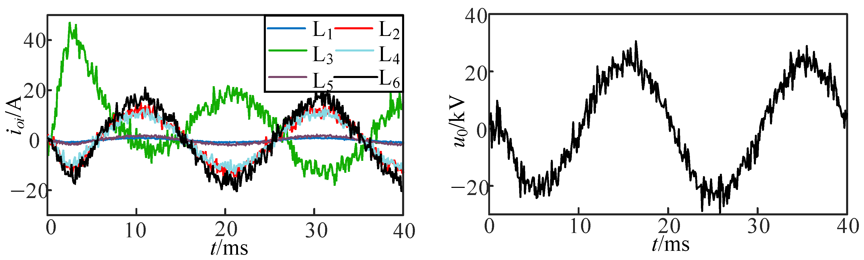
5.1.3. Noise Interference

To analyze the noise influence on fault signals in the actual operating environment of a distribution network, the reliability of the line selection method was evaluated by adding a 30 dB Gaussian white noise to the simulation signal. The line selection results are shown in

Table 5. Comparison of line selection results with noise and without noise.

Faulty Line	Fault Condition			Signal to Noise Ratio/dB	Inversion Correlation Coefficient Pk/P1, P2, P3, P4, P5, P6	Fault Line Discrimination Matrix s	Line Selection Result
	Rf/Ω	φ/(°)	Df/km
L1	500	0	10	0	9.8028, −0.0054, −0.0140 −0.0117, −0.0052, −0.0268	s = [−1 1 1 1 1 1]	Correct
L2	1000	60	5	30	−0.0226, 3.2850, −0.0220 −0.0104, 0.0241, −0.0198	s = [1 −1 1 1 1 1]	Correct
L3	1500	90	12	0	−0.0174, −0.0215, 2.5421 0.0103, −0.0163, 0.0210	s = [1 1 −1 1 1 1]	Correct
L4	2000	0	4	30	−0.3613, −0.0177, −0.0170 5.4078, −0.0242, −0.0165	s = [1 1 1 −1 1 1]	Correct
L5	2500	90	10	0	−0.0354, −0.0112, −0.0436, −0.0379, 4.0254, −0.0093,	s = [1 1 1 1 −1 1]	Correct
L6	3000	0	4	30	−0.0112, −0.0179, −0.0284, −0.0077, −0.0169, 4.0271,	s = [1 1 1 1 1 −1]	Correct
Bus bar	500	60	-	0	−0.0023, −0.0047, −0.0140 −0.0302, −0.0346, −0.0178	s = [−1 1 1 1 1 1]	Correct
Bus bar	3000	90	-	30	−0.0145, 0.0075, −0.0058 −0.0031, −0.0126, −0.0091	s = [−1 1 1 1 1 1]	Correct

, where D_f denotes the distance of a fault point. The current and voltage waveforms under the interference of 30 dB Gaussian white noise are shown in Figure 14.

Based on the results in Table 5, even after adding the 30 dB noise, the proposed method could accurately select fault lines and could identify bus faults without being affected by the noise environment.

To further validate the superiority of the proposed method in this paper, a comparative analysis was conducted between the proposed method and a fault section identification method based on PCA clustering analysis using instantaneous zero-sequence power from reference [22].

Considering that the zero-sequence power of feeders is directional, there are significant differences in the instantaneous zero-sequence power of each feeder after dimension reduction through principal component analysis (PCA). The faulted feeder can be identified based on the projection value of the instantaneous zero-sequence power on the first principal component axis (PC₁). Therefore, a fault section identification algorithm based on clustering discrimination can be constructed using this feature.

In the simulated model shown in Figure 4, three fault locations were set on feeder L₃ under the same fault conditions. After each fault occurrence, the instantaneous zero-sequence power of six feeders was extracted, resulting in a total of 18 samples of instantaneous zero-sequence power data. Since the instantaneous zero-sequence power undergoes significant changes after a fault, to avoid misidentification due to insufficient data collection, ten sampling points were selected to collect fault data. The instantaneous zero-sequence power was calculated using Equation (32), and an 18 × 10 matrix of instantaneous power ($\mathsf{\Delta }{p}_0$) was constructed.

$$\mathsf{\Delta }{p}_0=\left[\begin{array}{cccc}\mathsf{\Delta }{p}_{01}\left(1\right)& \mathsf{\Delta }{p}_{01}\left(2\right)& \dots & \mathsf{\Delta }{p}_{01}\left(10\right)\\ ⋮& ⋮& ⋮& ⋮\\ \mathsf{\Delta }{p}_{06}\left(1\right)& \mathsf{\Delta }{p}_{06}\left(2\right)& \cdots & \mathsf{\Delta }{p}_{06}\left(10\right)\\ ⋮& ⋮& ⋮& ⋮\\ \mathsf{\Delta }{p}_{18}\left(1\right)& \mathsf{\Delta }{p}_{18}\left(2\right)& \cdots & \mathsf{\Delta }{p}_{18}\left(10\right)\end{array}\right]$$

(32)

The instantaneous power matrix was subjected to PCA clustering analysis to determine the criteria for fault section identification based on clustering discrimination. If the projection of the instantaneous power on the PC₁ axis was $q_{{}_1}<0$, the line was identified as a faulted feeder. If the projection was $q_{{}_1}>0$, the line was identified as a healthy feeder.

Assuming that three different fault locations were set along feeder L₃, with a transition resistance of 500 Ω, a closing angle of 90°, and a sampling frequency of 10 kHz, a total of 18 samples of instantaneous zero-sequence power data were obtained from the six feeders, forming an instantaneous power matrix ($\mathsf{\Delta }{p}_0$). The clusters of feeder instantaneous power curves are shown in Figure 15.

The projection values on the PC₁ axis and the fault section identification results for different transition resistances set on feeder L₁ are shown in

Table 6. The fault section identification results under different fault transition resistances.

Rf/Ω	The Projection Values on the PC1 Axis	Results from Reference [22]	The Method Proposed in This Paper
50	(−0.6360, 0.1257, 0.1260, 0.1260, 0.1255, 0.1260)	Correct	Correct
100	(−0.5251, 0.1265, 0.1265, 0.1263, 0.1260, 0.1265)	Correct	Correct
300	(−0.6299, 0.1213, 0.1210, 0.1215, 0.1215, 0.1214)	Correct	Correct
500	(−0.6127, 0.1065, 0.1066, 0.1065, 0.1066, 0.1065)	Correct	Correct
800	(−0.6062, 0.1200, 0.1389, 0.1301, 0.1254, 0.1263)	Incorrect	Correct
1000	(−0.5983, 0.1176, 0.1209, 0.1187, 0.1236,0.1241)	Incorrect	Correct

. From Table 6, it can be observed that within the effective range of transition resistance, the faulted feeder has a negative projection value on the PC₁ axis, while the healthy feeders have positive projection values. The method proposed in reference [22] can effectively identify faulted feeders within a range of 800 m. However, beyond this range, the method proposed in this paper is more accurate.

6. Conclusions

The proposed method focuses on analyzing the dynamic behavior of a fault through an equivalent circuit that is specifically designed for HIG fault line selection in RGDN. By enhancing the accuracy of the line model during fault conditions, this method effectively identifies the faulty line by integrating voltage and current data from both high- and low-frequency ranges. The key findings of this study are summarized as follows:

• The fault detection algorithm is designed based on detecting sudden changes in the zero-sequence voltage. This algorithm effectively addresses issues such as incorrect operation of protection devices during high-resistance grounding faults, and failures of traditional fault detection algorithms when the initial phase angle of a fault is small and the transition resistance is large. As a result, the starting time of the line-selection device is shortened, and the overall sensitivity of the device is improved.
• The transient information of bus zero-sequence voltage and zero-sequence current on each line, analyzed in both high- and low-frequency bands, plays a crucial role in the selection of fault lines. This approach helps avoid problems such as missing fault information and low accuracy encountered when using only a single characteristic measure for selecting the fault line.
• The method being proposed offers prompt detection and response to HIG faults, eliminating the possibility of protection devices failing to operate. It also possesses extensive applicability. Moreover, it maximizes the utilization of fault information from each frequency band post-fault occurrence, enhances the fault characteristics, and accurately identifies the faulty line.

In the occurrence of a high-resistance grounding fault in a distribution network, the resistance value of the transition resistor typically ranges from several hundred to tens of thousands of ohms. As faults progress, the resistance value of the transition resistor will also vary, and the transient characteristics of the faults will diminish as the transition resistance increases. When the transition resistance exceeds 2 kilo-ohms or more, conventional line selection methods become impractical. Given the growing complexity of urban distribution networks, future endeavors will concentrate on the practical application of the methods proposed in this study.

References

1. Ghaderi, A.; Ginn, H.L.; Mohammadpour, H.A. High impedance fault detection: A review. Electr. Power Syst. Res. 2017, 143, 376–388. [Google Scholar] [CrossRef]
2. Gazzana, D.S.; Ferreira, G.; Bretas, A.S. An integrated technique for fault location and section identification in distribution systems. Electr. Power Syst. Res. 2014, 115, 65–73. [Google Scholar] [CrossRef]
3. Sedighizadeh, M.; Rezazadeh, A.; Elkalashy, N.I. Approaches in high impedance fault detection—A chronological review. Adv. Electr. Comput. Eng. 2010, 10, 114–128. [Google Scholar] [CrossRef]
4. Gautam, S.; Brahma, S.M. Detection of high impedance fault in power distribution systems using mathematical morphology. IEEE Trans. Power Syst. 2013, 28, 1226–1234. [Google Scholar] [CrossRef]
5. Silva, L.; Pereira, R.; Abbad, J.R. Optimised placement of control and protective devices in electric distribution systems through reactive tabu search algorithm. Electr. Power Syst. Res. 2008, 78, 372–381. [Google Scholar] [CrossRef]
6. Welfonder, T.; Leitloff, V.; Fenillet, R. Location strategies and evaluation of detection algorithms for earth faults in compensated MV distribution systems. IEEE Trans. Power Deliv. 2002, 15, 1121–1128. [Google Scholar] [CrossRef]
7. Baqui, I.; Zamora, I.; Mazon, J. High impedance fault detection methodology using wavelet transform and artificial neural networks. Electr. Power Syst. Res. 2011, 81, 1325–1333. [Google Scholar] [CrossRef]
8. Adamiak, M.; Wester, C.; Kulshrestha, A. High impedance fault detection on rural electric distribution systems. In Proceedings of the Rural Electric Power Conference, Orlando, FL, USA, 16–19 May 2010. [Google Scholar]
9. Ma, J.; Liu, J.; Deng, Z. An adaptive directional current protection scheme for distribution network with DG integration based on fault steady-state component. Int. J. Electr. Power Energy Syst. 2018, 102, 223–234. [Google Scholar] [CrossRef]
10. Sedighi, A.R.; Haghifam, M.R.; Malik, O.P. Soft computing applications in high impedance fault detection in distribution systems. Electr. Power Syst. Res. 2005, 76, 136–144. [Google Scholar] [CrossRef]
11. Han, L.; Liu, S.; Chen, H. A new method of fault line selection for resonant grounding system based on improved S transform parameters. In Proceedings of the 2019 IEEE Sustainable Power and Energy Conference (iSPEC), Beijing, China, 21–23 November 2019. [Google Scholar]
12. Song, X.; Gao, F.; Chen, Z. A negative selection algorithm based identification framework for distribution network faults with high resistance. IEEE Access 2019, 7, 109363–109374. [Google Scholar] [CrossRef]
13. Li, Y.; Meng, X.; Song, X. Single-phase-to-ground fault line detection for distribution network based on optimal finite impulse response filter and hierarchical clustering. Power Syst. Tech. 2015, 39, 143–149. [Google Scholar]
14. Shu, H.; An, N.; Yang, B. Single pole-to-ground fault analysis of MMC-HVDC transmission lines based on capacitive fuzzy identification algorithm. Energies 2020, 13, 319. [Google Scholar] [CrossRef]
15. Haghifam, M.R.; Sedighi, A.R.; Malik, O.P. Development of a fuzzy inference system based on genetic algorithm for high-impedance fault detection. IEE Power Gener. Transm. 2006, 153, 359–367. [Google Scholar] [CrossRef]
16. Jamali, S.; Bahmanyar, A. A new fault location method for distribution networks using sparse measurements. Int. J. Electr. Power Energy Syst. 2016, 81, 459–468. [Google Scholar] [CrossRef]
17. Wang, X.; Gao, J.; Wei, X. A novel fault line selection method based on improved oscillator system of power distribution network. Math. Probl. Eng. 2014, 10, 901810. [Google Scholar] [CrossRef]
18. Dong, X.; Shi, S. Identifying single-phase-to-ground fault feeder in neutral noneffectively grounded distribution system using wavelet transform. Electr. Power Sci. Eng. 2011, 23, 1829–1837. [Google Scholar]
19. Bakar, A.; Ali, M.S.; Tan, C.K. High impedance fault location in 11 kV underground distribution systems using wavelet transforms. Int. J. Electr. Power Energy Syst. 2014, 55, 723–730. [Google Scholar] [CrossRef]
20. Liu, M.; Fang, T.; Jiang, Y. A new correlation analysis approach to fault line selection based on transient main-frequency components. Power Syst. Prot. Control 2016, 44, 74–79. [Google Scholar]
21. Long, Y.; Ouyang, J.; Xiong, X. Single phase high resistance grounding protection of distribution network based on zero sequence power variation. Trans. China Electrotech. Soc. 2019, 34, 3687–3695. [Google Scholar]
22. Gao, F.; Zeng, L.; Li, Z. A new method for fault section identification in distribution networks combining distributed intelligent collaboration and cloud computing. Power Syst. Technol. 2021, 45, 2969–2978. [Google Scholar]
23. Shao, W.; Liu, Y.; Cheng, Y. High-resistance fault section identification method for resonant grounding systems based on zero-sequence impedance mutation characteristics. Electr. Power Autom. Equip. 2021, 41, 120–126. [Google Scholar]
24. Wang, B.; Cui, X.; Dong, X. Overview of arc high-resistance fault detection technology in distribution lines. Proc. Chin. Soc. Electr. Eng. 2020, 40, 96–107+377. [Google Scholar]
25. Wei, M.; Shi, F.; Zhang, H. High-resistance fault section identification and zone locating method for resonant grounding systems based on synchronous zero-sequence current harmonic group ratio phase. Proc. Chin. Soc. Electr. Eng. 2021, 41, 8358–8372. [Google Scholar]
26. Wang, X.; Gao, J.; Wei, X.; Guo, L.; Song, G.; Wang, P. Faulty feeder detection under high impedance faults for resonant grounding distribution systems. IEEE Trans. Smart Grid 2023, 14, 1880–1895. [Google Scholar] [CrossRef]
27. Xiao, Q.; Guo, M.; Chen, D. High-impedance fault detection method based on one-dimensional variational prototyping-encoder for distribution networks. IEEE Syst. J. 2022, 16, 966–976. [Google Scholar] [CrossRef]
28. Wang, B.; Cui, X. Nonlinear modeling analysis and arc high-impedance faults detection in active distribution networks with neutral grounding via Petersen coil. IEEE Trans. Smart Grid 2022, 13, 1888–1898. [Google Scholar] [CrossRef]
29. Wang, B.; Geng, J.; Dong, X. High-impedance fault detection based on nonlinear voltage–current characteristic profile identification. IEEE Trans. Smart Grid 2018, 9, 3783–3791. [Google Scholar] [CrossRef]
30. Huang, S.; Hsieh, C. High-impedance fault detection utilizing a Morlet wavelet transform approach. IEEE Trans. Power Deliv. 1999, 14, 1401–1410. [Google Scholar] [CrossRef]
31. Gao, J.; Wang, X.; Wang, X.; Yang, A.; Yuan, H.; Wei, X. A high-impedance fault detection method for distribution systems based on empirical wavelet transform and differential faulty energy. IEEE Trans. Smart Grid 2022, 13, 900–912. [Google Scholar] [CrossRef]
32. Tang, T.; Huang, C.; Jiang, Y. Fault line selection method in resonant earthed system based on transient signal correlation analysis under high and low frequencies. Power Syst. Autom. 2016, 40, 105–111. [Google Scholar] [CrossRef]
33. Grajales, E.; Mora, F.; Perez, L. Advanced fault location strategy for modern power distribution systems based on phase and sequence components and the minimum fault reactance concept. Electr. Power Syst. Res. 2016, 140, 933–941. [Google Scholar] [CrossRef]
34. Xue, Y.; Li, J.; Chen, X. Faulty feeder selection and transition resistance identification of high impedance fault in a resonant grounding system using transient signals. Proc. CSEE 2017, 37, 5037–5048+5223. [Google Scholar]
35. Russell, B.; Benner, C. Arcing fault detection for distribution feeders: Security assessment in long term field trials. IEEE Trans. Power Deliv. 1995, 10, 676–683. [Google Scholar] [CrossRef]
36. Cohen, J. Statistical Power Analysis for the Behavioral Sciences, 2nd ed.; Lawrence Erlbaum Associates: Hillsdale, NJ, USA, 1988. [Google Scholar]
37. Li, S.; Gao, G.; Hu, G.; Gao, B.; Gao, T.; Wei, W.; Wu, G. Aging feature extraction of oil-impregnated insulating paper using image texture analysis. IEEE Trans. Dielectr. Electr. Insul. 2017, 24, 1636–1645. [Google Scholar] [CrossRef]
38. Xue, Y.; Li, J.; Xu, B. Transient equivalent circuit and transient analysis of single-phase earth fault in arc suppression coil grounded system. Proc. CSEE 2015, 35, 5703–5714. [Google Scholar]
Figure 1. Transient equivalent circuit of resonant grounding system.
Electronics 12 04066 g001
Figure 2. Equivalent circuit of high-resistance grounding fault.
Electronics 12 04066 g002
Figure 3. Simplified zero-sequence network.
Electronics 12 04066 g003
Figure 4. Simulation model of high-resistance grounding fault.
Electronics 12 04066 g004
Figure 5. Comparison of zero-sequence current of feeder under different transition resistances.
Electronics 12 04066 g005
Figure 6. Zero-sequence voltage and its gradient sum.
Electronics 12 04066 g006
Figure 7. A 15%Um start.
Electronics 12 04066 g007
Figure 8. Zero-sequence voltage gradient sum start.
Electronics 12 04066 g008
Figure 9. Zero-sequence voltage gradient sum start at K = 5.
Electronics 12 04066 g009
Figure 10. Transient signal in low-frequency band when fault initial phase angle is 0°.
Electronics 12 04066 g010
Figure 11. Transient signal in low-frequency band when fault initial phase angle is 90°.
Electronics 12 04066 g011
Figure 12. Line selection process.
Electronics 12 04066 g012
Figure 13. Feeder zero-sequence current and bus zero-sequence voltage.
Electronics 12 04066 g013
Figure 14. Feeder zero-sequence current and bus zero-sequence voltage after adding noise.
Electronics 12 04066 g014
Figure 15. The clusters of instantaneous zero-sequence power curves for each feeder within a certain time window.
Electronics 12 04066 g015