1. Introduction
In the dynamic realm of vehicular technology, inter-vehicular communications serve as a foundational pillar, driving advancements in road safety, traffic management, and passenger experience. Enabled by Vehicular Ad-Hoc Networks (VANETs) [
1], these communications are facilitated through On-Board Unit (OBU) devices that vehicles are equipped with. The primary communication paradigms include Vehicle-to-Vehicle (V2V) and Vehicle-to-Infrastructure (V2I). The V2I paradigm relies on strategically placed Roadside Units (RSUs) to ensure uninterrupted data packet transmission. However, the dynamic nature of VANETs, marked by frequent topological changes due to vehicular speeds and mobility, poses challenges in data transmission. These challenges include intermittent connection disruptions, interference in high-traffic areas, and signal attenuation due to obstacles. A significant concern is the potential for delay in data packet transmission from an emergency vehicle, which could jeopardize a patient’s timely arrival at a medical facility. While there is extensive literature on channel characterization across urban, rural, and suburban areas [
2,
3,
4,
5,
6], only a few have explored the potential of ANN, stochastic models, and machine learning for channel modeling [
7,
8,
9,
10]. For example, Ref. [
10] presents a detailed physical layer simulation tool in Simulink, specifically designed for vehicular communication modeling.
1.1. Problem Statement
The central challenge revolves around ensuring reliable data packet transmission paths, especially for emergency vehicles traversing intricate urban landscapes. Buildings and other infrastructural elements can significantly weaken signals, resulting in transmission errors. While traditional models offer some solutions, they may not fully capture the complexities of urban environments. This underscores the need for an advanced solution capable of accurately predicting transmission errors, thus facilitating proactive measures to maintain seamless communication.
1.2. Contributions
Our research tackles the aforementioned challenge through the following key contributions:
ANN-based BER Estimation: We propose a novel model utilizing artificial neural networks to predict the Bit Error Rate (BER) based on the characteristics of nearby buildings.
Incorporation of Environmental Characteristics: Our model integrates building information (, , , ) and the physical attributes of the environment, including the antenna parameters of vehicles, as reflected in the NS-3 physical layer.
Data Collection: We employ Network Simulator 3 (NS-3) alongside the SUMO mobility simulator to extract real-world geospatial data from the OpenStreetMap geographic database, capturing the 2D geometric structure of buildings for our ANN.
Algorithm Assessment: We assess the efficacy of ten distinct learning algorithms for our ANN using five pivotal metrics, highlighting the superior performance of the Conjugate Gradient With Powell/Beale Restarts (CGB) learning algorithm.
Enhanced Communication Reliability: Our research augments the reliability of communication in urban VANET contexts, especially for emergency vehicles, by leveraging supervised learning and ANNs to predict signal degradation and optimize routing decisions.
The remainder of this paper is organized as follows:
Section 2 provides a comprehensive literature review, focusing on relevant research in the field.
Section 3 introduces artificial neural networks, highlighting their significance and application in our study. In
Section 4, we detail the step-by-step process employed to develop the BER estimation model. Subsequently,
Section 5 presents the obtained results, accompanied by a meticulous analysis. Finally,
Section 6 concludes the paper, summarizing the key findings and discussing potential avenues for future research.
2. Related Work
The past decade has seen significant advancements in the realm of vehicular communications, with researchers exploring various facets of signal propagation, channel estimation, and path loss prediction, especially in urban vehicular environments. A prominent study by Ding and Ho presented a digital-twin-enabled deep learning approach, which combined a digital representation of the real-world system with deep learning, outperforming existing methodologies in dynamic urban vehicular environments [
11]. Similarly, a deep learning-based channel estimation methodology for Vehicle-to-Everything (V2X) communications has been proposed, addressing the rapid time variations and non-stationary characteristics of wireless channels [
12]. Wang and Lu demonstrated the practical constraints of translating physical-layer network coding theories integrated with deep neural networks into real-world applications for vehicular ad-hoc networks [
13].
Path loss prediction has been another area of focus. Zhang et al. [
14] introduced a comprehensive exploration of machine-learning-driven path loss prediction, highlighting the superior performance of machine-learning models compared to traditional models. Jo et al. [
15] further advanced this by synergizing three pivotal techniques, ANN, Gaussian process, and PCA, for feature selection, presenting a holistic machine-learning framework for path loss modeling. Aldossari [
16] explored the challenges of signal propagation in indoor environments, especially within the realm of 5G, proposing a data-driven approach leveraging artificial intelligence.
Vehicular Ad-Hoc Networks (VANETs) have also been extensively researched. Liu, St. Amour, and Jaekel focused on the transmission of basic safety messages in VANETs, proposing a reinforcement learning-based congestion control approach [
17]. Turan and Coleri emphasized the potential of vehicular visible light communication as a V2X communication method, introducing a machine-learning framework for improved path loss modeling [
18]. Moreover, Ramya et al. [
19] proposed a non-parametric, data-driven approach using the Random Forest learning method for V2V path loss prediction.
Signal strength prediction is also a critical domain. Igwe et al. [
20] introduced a methodology harnessing the power of ANNs to compute received signal strength based on atmospheric parameters. Thrane et al. [
21] further explored this by leveraging satellite imagery with deep learning for signal strength prediction. Bahramnejad and Movahhedinia presented an analytical framework for estimating the reliability of V2V communications within cognitive radio-VANETs, integrating a Markov model and an ANN model for streamlined reliability estimation [
22].
Although these studies have made significant advancements within their respective domains, our present work distinguishes itself by focusing on signal degradation in urban VANETs. Our approach employs supervised learning anchored in ANNs to estimate signal degradation based on obstacles encountered by moving vehicles.
Table 1 concisely summarizes these studies based on their focus areas, primary methodologies, and applicability, particularly within the urban VANET context:
3. Artificial Neural Networks
Artificial Neural Networks (ANNs) are powerful models for statistical learning, drawing inspiration from the intricate workings of biological neural networks. ANNs have gained significant popularity within machine learning [
23]. Several research papers [
24,
25] in the realm of medicine harness artificial neural networks to address a diverse range of challenges. These networks are composed of interconnected “neurons” that communicate with each other via synapses, mimicking the neural connections found in living organisms. The strength of these connections is adaptively modified based on input and output signals, making ANNs highly suitable for supervised learning tasks.
A typical neural network comprises three essential components: the input layer, the hidden layer(s), and the output layer. This structure can be envisioned as a black box, as illustrated in
Figure 1 below, encapsulating the intricate computations performed by the network. The input layer receives the initial data, which is then processed through the interconnected hidden layer(s), ultimately producing an output through the output layer.
4. Supervised Learning for Estimating the Bit Error Rate (BER)
In this section, we present our approach for applying supervised learning to address our research problem. Our approach encompasses seven key steps, outlined as follows:
4.1. Data Collection
The data collection phase is crucial for establishing a comprehensive knowledge base for machine learning. In our study, data are collected through simulations, enabling us to obtain essential information. This includes the geometric structure of the building (, , , ), the signal-to-noise ratio, the number of transmitted and received bits, the percentage of received bits, and the Bit Error Rate (BER). These collected data points serve as the foundation for our subsequent machine-learning analyses.
4.1.1. Experimental Environment for Data Collection
The experimental environment used for data collection consists of two simulators: a network simulator and a traffic simulator. To enable comprehensive studies based on the protocols under analysis, we chose NS-3 (Network Simulator 3) [
26] as our network simulator. NS-3 offers a wide range of network components that facilitate diverse investigations in the field of wireless network technologies [
27]. Moreover, NS-3 supports essential standards such as IEEE 802.11 PHY/MAC [
28], 1609/WAVE [
29], and 802.11p [
30,
31], enabling realistic studies on Vehicular Ad Hoc Networks (VANETs). Furthermore, NS-3 provides support for Dedicated Short Range Communication (DSRC) [
32], a technology widely employed in North America for real-world vehicle communications testing.
To incorporate a mobility model specific to vehicles, we opted to utilize SUMO (Simulation of Urban MObility) [
33] as our traffic simulator. SUMO is a frequently employed tool in studies related to traffic analysis in road networks. Additionally, SUMO offers the capability to interact with external applications through a socket connection. This interaction is facilitated by TraCi (Traffic Control Interface), enabling simulations in a client/server mode.
Figure 2 shows a visual representation of our experimental environment.
4.1.2. Experiment Scenarios for Data Gathering
This subsection provides a concise overview of the approach employed to specify urban scenarios using the SUMO simulation framework. Within SUMO, a range of tools was utilized to define the urban components, including obstacles such as buildings.
Figure 3 illustrates the process of generating urban scenarios in SUMO.
In our study, it was crucial to accurately represent the geometric structure of the network, considering urban elements such as buildings. To accomplish this, we leveraged the capabilities of the NETCONVERT and POLYCONVERT tools provided by the SUMO traffic simulator.
The NETCONVERT tool facilitated the conversion of files (e.g., OSM) containing information about the geometric structure of road networks from diverse sources into a format compatible with SUMO. Specifically, for our research, we imported the specifications of the geometric structure of the road network from the OpenStreetMap platform [
34].
The POLYCONVERT tool was employed to transform the geometric forms (i.e., buildings) obtained from various sources into a visualizable representation within the graphical interface of SUMO.
After defining the urban model, the next step is to develop a script in NS-3 that builds upon this model.
4.1.3. Examples of Urban Model Specification Using SUMO
In this subsection, we present two illustrative examples of urban model specification using SUMO.
Signal Degradation between Two Vehicles Due to Obstacle Presence
The specific scenario can be described as follows: At time instant
, two vehicles,
and
, act as the transmitter and receiver, respectively, and are located on a road segment. At
, the transmission between
and
is disrupted due to the presence of an obstacle. This scenario effectively demonstrates the impact of obstacles, such as walls or buildings, on signal degradation. To quantify the extent of signal degradation caused by an obstacle, our study focuses on the transmission between these two vehicles. By limiting the transmission to only two vehicles, we aim to gain a deeper understanding of the obstacle’s impact on the signal degradation phenomenon.
Figure 4 below visually depicts the aforementioned scenario using SUMO.
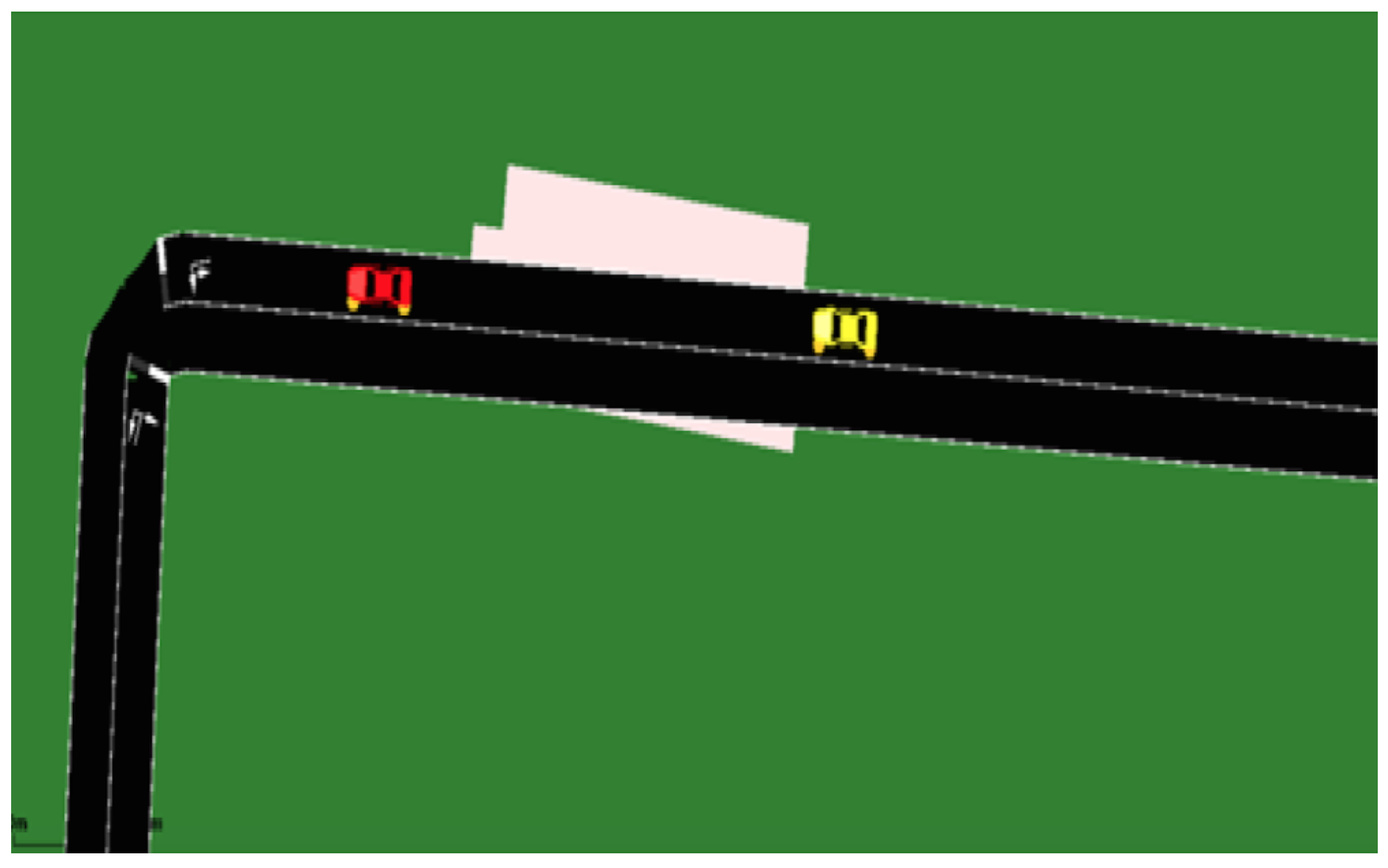
Signal Degradation Between Two Vehicles Caused by Bridge Presence
In this scenario, we consider two vehicles located within transmission range, traversing a two-lane bridge. The communication signal between these vehicles experiences attenuation due to the presence of the bridge. This scenario emphasizes the phenomenon of signal attenuation in an enclosed space.
Figure 5 below depicts the described scenario, illustrating the signal attenuation caused by the presence of the bridge.
In
Figure 4 and
Figure 5, the vehicles
and
are depicted in red and yellow, respectively. The pink illustrations represent the obstacles that obstruct the transmission signal between
and
.
4.1.4. NS-3 Simulation Parameters for Data Collection
In this section, we provide a summary of the simulation parameters used in NS-3 to establish the foundational knowledge for our learning system.
Table 2 presents the experiment parameters utilized in the NS-3 simulations.
Furthermore,
Table 3 demonstrates a sample of the simulation results, highlighting the obtained data.
Figure 6 illustrates the representation of an obstacle in our urban scenarios.
Where = , = , = , and =
Table 3 demonstrates how each geometric structure of a building impacts the transmission quality. This information can be interpreted through qualitative variables such as SNR and BER.
4.2. Data Preprocessing
During this stage, we undertake data preprocessing to optimize the usability of input and output parameters for the learning algorithm. Our preprocessing strategy entails removing superfluous details, notably the inclusion of the quantity of received bits and the corresponding percentage of received bits. While these details are related to the predicted variable (Bit Error Rate or BER), they are identified as non-essential for the learning system. By eliminating these extraneous details, we refine the dataset to facilitate more efficient analysis and model training.
Moreover, we standardize our data using the Min–Max normalization technique. This approach enables us to perform a linear conversion on the original data within the range of 0 to +1, employing the following formula:
where:
X is the original value;
is the minimum value in the dataset;
is the maximum value in the dataset;
is the normalized value.
4.3. Choice of Learning Function
In this section, we explore the process of selecting an appropriate learning function for our model. It is important to note that our selection is limited to the ten algorithms available in MATLAB 2016a, as this is the version we are using. To determine the most suitable option, we employ statistical indicators such as Mean Absolute Error (MAE), Mean Squared Error (MSE), Root Mean Squared Error (RMSE), Correlation Coefficient (R), and Maximum Prediction Error (MaxPE) to evaluate the effectiveness of each machine-learning function. A comprehensive assessment of these learning functions, all of which were tested using MATLAB, is provided in
Table 4.
The Mean Absolute Error (MAE) quantifies the average magnitude of the absolute differences between the observed and forecasted values in the dataset. It provides a measure of the residuals present in the dataset:
The Mean Squared Error (MSE) represents the mean of the squared differences between the actual and predicted values within a dataset. This metric gauges the extent of variance in the residuals:
The Root Mean Squared Error (RMSE) is the square root of the Mean Squared Error, serving as a metric to gauge the standard deviation of residuals:
The Correlation Coefficient (R) quantifies the relationship between two variables. As the value of the index approaches +1, the stronger the positive association between the variables in question becomes:
The Maximum Prediction Error (MaxPE) represents the largest discrepancy between the observed and predicted values. It serves as a metric to gauge the maximum error in predictions:
where:
is the observed value;
is the predicted value;
and are the mean of the observed and predicted data points, respectively;
n is the number of data points.
Following our assessment, we have opted for the Conjugate Gradient with Powell/Beale Restarts learning function for our model owing to its performance, as evidenced by its recorded lowest MAE, MSE, RMSE, MaxPE, and higher R values. To gain a visual understanding of how the various learning functions perform based on the aforementioned metrics, please consult
Figure 7 provided below.
4.4. Data Splitting for Training, Testing, and Validation
To ensure proper evaluation and validation of our model, the gathered data are split into distinct subsets. This step allows for the allocation of data for training, testing, and validation purposes, ensuring robust performance assessment. The following example illustrates the distribution of the data:
70% of the data is allocated for the learning phase;
15% of the data is reserved for validation purposes;
Another 15% is dedicated to testing the model’s performance.
4.5. Model Evaluation
The evaluation step plays a crucial role in assessing the model’s capabilities using data that have not been previously utilized for learning. By subjecting the model to this independent dataset, we gain valuable insights into its real-world potential and how it would perform in practical scenarios.
4.6. Tuning Model Parameters
After evaluating the model, we engage in fine-tuning the learning process to enhance its performance. This step involves adjusting specific parameters within the model, such as the number of neurons, learning functions, and synaptic weights, among others. By iteratively refining these parameters, we can optimize the model’s learning process and achieve improved overall performance.
4.7. Estimation of Bit Error Rate (BER)
In this step, we leverage the trained model to estimate the Bit Error Rate (BER) based on new data. Specifically, we feed 300 new samples into the model, which then generates an output corresponding to the estimated BER value.
5. Results and Analysis
In this section, we present the outcomes and provide an in-depth analysis resulting from the evaluation of our developed model.
5.1. Results
The results are presented in tabular format, highlighting the model’s accuracy based on criteria such as MSE, RMSE, MAE, MaxPE, and R.
5.1.1. Parameter Selection for the Developed Neural Network Model
To configure the developed neural network, we carefully determined the parameters for optimal performance. The architecture of the model consists of eighteen hidden layers, as depicted in
Figure 8. We divided the dataset into three subsets, allocating 70% for the learning phase, 15% for validation, and the remaining 15% for testing purposes. The following results were obtained using this specific configuration.
Table 5 below highlights the network accuracy with 18 hidden neurons.
5.1.2. Adjusting the Number of Hidden Neurons
To investigate the impact of varying the number of hidden neurons on the network’s performance, we conducted experiments using different configurations. To ensure consistency, the distribution of the entire learning dataset in the subsequent results was kept consistent with the default values (70% for learning, 15% for validation, and 15% for testing), while only the number of hidden neurons was altered.
Table 6 below highlights the network accuracy.
5.2. Analysis
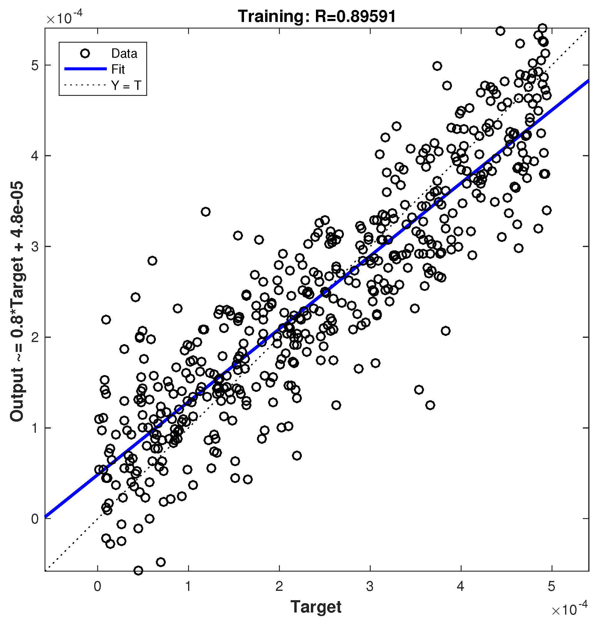
The results presented in
Figure 9 and
Figure 10 illustrate the regression plots for learning with 18 and 45 neurons, respectively. The correlation coefficient (R) is a measure of the relationship between the network outputs and the targets. A correlation coefficient close to 1 indicates good learning, while a value close to 0 indicates weak learning.
Regression plots provide a visual representation of the network outputs compared to the targets across learning, validation, or test datasets. A perfect fit occurs when the data points align along the 45-degree line, indicating that the network outputs perfectly match the targets. In our study, the learning process achieved a correlation coefficient of R = 0.89591 when using 18 hidden neurons and R = 0.99979 when using 45 hidden neurons. These values indicate a strong performance in terms of learning.
Figure 11 and
Figure 12 demonstrate the impact of varying the number of hidden neurons on the estimated Bit Error Rate (BER) value. When using 45 hidden neurons, the correlation coefficient indicates good learning performance (R = 0.99979) compared to the network trained with 18 hidden neurons (R = 0.89591). However, the model’s generalization capacity, which refers to its ability to perform well on unseen data, diminishes when using 45 neurons, as depicted in
Figure 12. In contrast, the model trained with 18 neurons (
Figure 11) exhibits greater precision, with errors ranging between −1 and 1. Conversely, the model trained with 45 neurons loses precision, leading to higher error values. This phenomenon is attributed to overfitting, where an increase in hidden neurons improves the learning process but compromises the accuracy of the model.
Thus, depending on the specific problem being studied, it is crucial to strike a balance between learning performance and model accuracy. In our case, the results indicate that the model based on 18 hidden neurons achieves a better compromise between the two. Consequently, for optimal prediction performance, it is recommended to calibrate the network with 18 hidden neurons.
In conclusion, based on our analysis, using 18 hidden neurons yields superior prediction performance in our case study.
6. Conclusions
In this paper, we presented an empirical study based on neural networks that estimates the BER in relation to obstacles (primarily buildings) encountered by a mobile vehicle in a VANET network. This study is driven by the need for Quality of Service (QoS) in emergency communications within VANETs. By estimating the BER based on the geometric structure of obstacles, vehicles can optimize their data routing decisions more effectively.
For our future work, we plan to integrate the mechanism for BER estimation with the CL-ANTHOCNET routing protocol we previously developed [
35]. Subsequently, we will evaluate its performance in scenarios involving the transmission needs of emergency vehicles.


