Three-Dimensional Point Cloud Reconstruction Method of Cardiac Soft Tissue Based on Binocular Endoscopic Images

Abstract

Three-dimensional reconstruction technology based on binocular stereo vision is a key research area with potential clinical applications. Mainstream research has focused on sparse point reconstruction within the soft tissue domain, limiting the comprehensive 3D data acquisition required for effective surgical robot navigation. This study introduces a new paradigm to address existing challenges. An innovative stereoscopic endoscopic image correction algorithm is proposed, exploiting intrinsic insights into stereoscopic calibration parameters. The synergy between the stereoscopic endoscope parameters and the disparity map derived from the cardiac soft tissue images ultimately leads to the acquisition of precise 3D points. Guided by deliberate filtering and optimization methods, the triangulation process subsequently facilitates the reconstruction of the complex surface of the cardiac soft tissue. The experimental results strongly emphasize the accuracy of the calibration algorithm, confirming its utility in stereoscopic endoscopy. Furthermore, the image rectification algorithm exhibits a significant reduction in vertical parallax, which effectively enhances the stereo matching process. The resulting 3D reconstruction technique enables the targeted surface reconstruction of different regions of interest in the cardiac soft tissue landscape. This study demonstrates the potential of binocular stereo vision-based 3D reconstruction techniques for integration into clinical settings. The combination of joint calibration algorithms, image correction innovations, and precise tissue reconstruction enhances the promise of improved surgical precision and outcomes in the field of cardiac interventions.

1. Introduction

Binocular stereo vision is derived from human eyes. In 1979, Marr and Poggio et al. [1] proposed and verified a computational model and algorithm inspired by the human stereo vision system, marking a significant milestone in the field of computer vision. Since then, binocular stereo vision has evolved into an indispensable component within the realm of computer vision. Binocular stereo vision leverages a pair of cameras to concurrently capture two-dimensional images of the same scene from various angles. Initially, a computer-based matching process is employed to derive the parallax image by aligning and comparing the two images. Then, the surface three-dimensional point cloud information is acquired, utilizing the binocular camera parameters via the relevant calculation. Finally, the three-dimensional reconstruction of the relevant scene is accomplished. Due to its uncomplicated apparatus and user-friendly operation, binocular stereo vision finds extensive utilization in domains such as robotic vision, industrial metrology, medical data processing, and related disciplines [2,3].

Camera calibration is an indispensable part of binocular stereo vision [4]. The acquisition of parameter information through camera calibration is a prerequisite for utilizing the disparity information of matched points to derive their actual coordinates within the three-dimensional scene. Camera calibration is the prerequisite and basis for the smooth acquisition of 3D point cloud information. Since its development, camera calibration methods have varied. However, these methods can be broadly classified into three main categories: traditional camera calibration methods, active vision calibration methods, and camera self-calibration methods.

In recent years, the field of surgical robotics has witnessed rapid advancement and extensive utilization, driven by continuous advancements in science and technology. The operative end of surgical robots incorporates a stereo endoscope, comprising two monocular endoscopes, thereby forming a binocular system. However, this operational mode possesses a notable drawback whereby the perception of depth information relies on the surgeon’s visual interpretation, lacking access to real, precise three-dimensional measurement data. Therefore, additional work is required to improve image accuracy in surgical vision [5,6,7]. Consequently, the direct provision of accurate three-dimensional measurement data to the surgical robot system remains unachievable, thus impeding the progress of surgical robots in attaining enhanced intelligence.

With environmental pollution and population aging, the incidence of cardiovascular diseases is increasing. In the present research landscape, binocular 3D reconstruction technology is still one of the current research hotspots [8,9]. However, several challenges persist, particularly in the realm of dense point reconstruction within soft tissue, where limited studies have been conducted [10]. This limitation impedes the attainment of comprehensive intraoperative guidance for surgical robots, as only the interest surface can be attained [11]. Therefore, the study of stereoscopic endoscope calibration [12,13] and image correction technology [14,15] has important practical significance.

The stereoscopic endoscope serves as an equivalent binocular stereo vision system, offering the potential to acquire three-dimensional measurement data of a lesion area’s surface based on the obtained stereo images. In the medical field, there is an urgent demand to enhance the perception of surgeons and surgical robots during procedures through the three-dimensional reconstruction of the lesion area’s surface. Visual tracking utilizing a stereo endoscope emerges as the optimal solution to establish a more stable surgical environment. To achieve successful visual tracking, obtaining accurate 3D measurement data on the target area necessitates the reconstruction of the specific region of interest on the heart’s soft tissue surface. This study provides significant contributions in the following aspects:

We propose a novel joint calibration algorithm for stereo endoscopes, leveraging a single-camera approach employing a checkerboard plane template.

A stereo endoscopic image correction algorithm is designed based on the known stereoscopic endoscopic parameters, which correct the stereoscopic image, employing parameter reconstruction, back projection, rotation, de-distortion, re-projection, and bilinear interpolation.

The 3D reconstruction of the surface of heart soft tissue includes the 3D reconstruction of spatial points and surface reconstruction, and obtaining the 3D points according to the stereo endoscopic parameters and the disparity map between the heart soft tissue images. After filtering and point cloud streamlining, the 3D points are then triangulated to achieve the surface reconstruction of the heart soft tissue.

2. Related Work

2.1. Binocular Stereo Vision Camera Calibration

Scholars have proposed some calibration methods with good performances, including using typical traditional cameras. One calibration method is the plane template method first proposed by Professor Zhang Zhengyou [16] in 1999. It is currently the most widely used calibration algorithm. In terms of camera self-calibration, scholars have also proposed some better self-calibration methods [17,18]. These all promote the continuous improvement of camera calibration methods.

Direct linear calibration algorithms are widely used in camera calibration tasks [19]. This algorithm is based on a linear imaging model. By establishing the correspondence between the 3D coordinates of the points within a three-dimensional scene and the pixel coordinates of their corresponding points in the image, a linear calibration is obtained. By solving this linear equation, the camera parameters can be obtained. The solution process is fast and straightforward. However, this method ignores lens distortion during the camera imaging process, so there is a certain error in the calibration result. To solve the problem of lens distortion, Kwon, Y.-H [20] proposed and verified a calibration method based on nonlinear optimization. However, the algorithm solution process is more complicated, and too many iterations make the running time longer. It is long, and there are certain unstable factors. For example, suppose the initial parameters substituted in the iterative process are not appropriate. In that case, the result will be very large, or the result will not converge. To combine the two calibration methods of linear and non-linear optimization, in the mid-1980s, the “Tsai” two-step method was proposed to realize camera calibration [21]. The algorithm exhibits superior computational speed and accuracy. However, it solely considers the radial distortion, leading to some degree of deviation in the calibration outcomes. Subsequently, numerous algorithms have emerged, employing enhanced techniques as their basis. In addition, various self-calibration methods tailored to different scenarios have been proposed. Nonetheless, while this calibration approach offers convenience, its robustness falls short when compared to alternative calibration algorithms.

2.2. Stereo Endoscope Vision and 3D Reconstruction

The stereoscopic endoscope is equivalent to a binocular stereo vision system. In theory, the stereo endoscope’s stereo image can obtain 3D measurement data corresponding to a lesion area’s surface [22,23]. The 3D reconstruction of the lesion surface is also an urgent need in the medical neighborhood to enhance doctors’ and surgical robots’ perceptions of surgery [24]. Illustratively considering robot-assisted coronary artery bypass grafting surgery, the surgical target encompasses a dynamically pulsating heart. Nonetheless, the intrinsic dynamism of the beating heart presents substantial procedural complexities. Scholars have proposed the notion of “heart rate synchronization,” which involves monitoring the motion of the cardiac surface and actively regulating the movements of the robotic manipulator to align with it. Consequently, this approach fosters the establishment of a more steadfast surgical environment, enhancing the operating conditions for surgeons [25]. Visual tracking based on the stereo endoscope is undoubtedly the best scheme to realize this idea. The premise of visual tracking is to obtain the corresponding region’s 3D measurement data. Therefore, it is necessary to reconstruct the interest block area on the heart’s soft tissue surface to obtain accurate 3D measurement data.

Foreign scholars have conducted some research on stereo endoscope vision. They achieved a semi-dense 3D reconstruction via structure propagation. Penza and colleagues [26] presented an advanced strategy for 3D reconstruction, utilizing a sliding window approach and census transform characteristics. In recent years, Guang Zhong Yang et al. [27] of Imperial College London have been devoted to research on the surgical navigation of stereoscopic endoscope vision and have also carried out much research in this field, and achieved certain results [28,29].

Overall, while stereo endoscopes 3D reconstruction has demonstrated progress, a substantial gap still remains before its clinical application becomes feasible. Presently, the predominant focus of the research in soft tissue 3D reconstruction lies in sparse point reconstruction, which falls short of obtaining comprehensive 3D measurement data for the corresponding surfaces. Consequently, effective guidance for surgical robots cannot be fully achieved.

3. Dataset

In the experiment, the binocular camera to be calibrated is a parallel placement structure. Thus, the resolution of both cameras is $658\times 429$, the $12\times 8$ calibration template is a dichromatic checkerboard, and the side length of the square is 18 mm, as shown in Figure 1.

As is presented in Figure 2, in the stereoscopic endoscopic image correction experiment, the dataset used comes from the actual cardiac soft tissue stereo image provided by Imperial College London.

4. Method

The camera imaging model transforms 3D scene information into the optical geometric imaging of plane images through geometric projection and photoelectric conversion [30,31]. Ideally, there is a certain deviation between the obtained stereo images [32], thereby necessitating the application of image correction techniques. This correction process aims to alleviate the vertical parallax present in the stereo image [33,34].

The heart’s soft tissue surface 3D reconstruction involves utilizing the dense parallax map and stereo endoscope parameters to derive three-dimensional spatial coordinates of the corresponding points, enabling the subsequent surface reconstruction based on the acquired three-dimensional point cloud data.

4.1. Joint Calibration Algorithm

As shown in

Table 1. Parameters required for stereoscopic endoscopes.

Parameter	Expression
Right and left parameter matrix $A_l$$, A_r$	$A=\left[\begin{array}{ccc}{f}_x& \gamma & u_0\\ 0& f_y& v_0\\ 0& 0& 1\end{array}\right]$
Radial distortion and tangential distortion	$k_1$$, k_2$$, p_1$$, p_2$
External parameters (rotation matrix and translation vector)	$R=\left[\begin{array}{ccc}{r}_1& r_2& r_3\\ r_4& r_5& r_6\\ r_7& r_8& r_9\end{array}\right]$$, T=\left[\begin{array}{c}{t}_1\\ t_2\\ t_3\end{array}\right]$

, the joint calibration of the stereoscopic endoscope is to obtain the internal parameter matrices $A_l$ and $A_r$ of the two endoscopes; the respective distortion parameters $k_1$, $k_2$ $p_1$, $p_2$; the external parameters, denoted as $T$ and $R$, represent the translation vector and rotation matrix that characterize the spatial relationship between the coordinate systems of the two endoscopes.

For the stereoscopic endoscopes, the tangential distortion coefficient is introduced. Consequently, we set the initial values for the tangential distortion coefficients $p_1$, $p_2$ to zero. We combined the obtained endoscope parameters to establish a minimization model, as shown in Equation (1):

$$\sum _{\mathrm{i}=1}^n \sum _{j=1}^m ∥m_{i\mathrm{j}}-\widehat{m}\left(A,k_1,k_2,p_1,p_2,R_i,T_i,M_j\right)∥$$

(1)

Among them, ${\mathrm{m}}_{\mathrm{ij}}$ represents the actual pixel positions of the j-th corner on the i-th image. $\widehat{m}\left(A,k_1,k_2,R_i,T_i,M_j\right)$ is the pixel positions of the j-th corner on the i-th image obtained via calculation. Matrix $T_i$ is translation vector. Parameters $k_1$, $k_2$ are the radial distortion coefficients. Matrix $R_i$ is the rotation matrix.

Upon the completion of both endoscopes’ calibration process, $T_i$ and $R_i$ characterize the relationship between the endoscopes and the world coordinate systems corresponding to the template are derived.

We denoted $R_i$ and $T_i$ for the left endoscope as ${\mathrm{R}}_{\mathrm{l}}$ and ${\mathrm{T}}_{\mathrm{l}}$, and for the right endoscope as $R_r$ and $T_r$, respectively.

If there is a $Q \left(X_w, Y_w, Z_w\right)$ within the calibration template, its coordinates in the right and left endoscope systems are denoted as $Q \left(X_r, Y_r, Z_r\right)$ and $Q \left(X_l Y_l, Z_l\right)$.

Equations (2) can be obtained according to their projection relationship.

$$\left[\begin{array}{l}{X}_l\\ Y_l\\ Z_l\\ 1\end{array}\right]=\left[\begin{array}{cc}{R}_l{R}_r^{-1}& T_l-R_l{R}_r^{-1}{T}_r\\ 0& 1\end{array}\right]\left[\begin{array}{l}{X}_r\\ Y_r\\ Z_r\\ 1\end{array}\right]=\left[\begin{array}{cc}R& T\\ 0& 1\end{array}\right]\left[\begin{array}{l}{X}_r\\ Y_r\\ Z_r\\ 1\end{array}\right]$$

(2)

Among them, the rotation matrix $R=R_l{R}_r^{-1}$ and the translation vector $T=T_l-R_l{R}_r^{-1}{T}_r$ represent the transformation of the coordinate system of the right endoscope to the left one. $T$ and $R$ serve as the external parameters of the stereoscopic endoscope to be solved.

4.2. Binocular Endoscope Image Matching Algorithm

In actual situations, there are certain differences between the internal parameters of the two endoscopes. The actual epipolar geometric relationship between the two images is visually depicted in Figure 3.

In Figure 3, $O_{cl}$ is the optical center of the left endoscope, and $O_{cr}$ is the optical center of the right endoscope. M is the observed space point. $m_l$ and $m_r$ are the projection points of M on the left and right images, respectively.

The $L_l$ and $L_R$ in the figure are the epipolar lines of the left and right cameras, respectively. Due to the non-collinearity of the epipolar lines in the left and right images, it is crucial to establish the appropriate epipolar equation in the right image based on the image point of the left image before conducting the stereo matching operation. This enables the subsequent search for the matching point along the designated epipolar line.

After the calibration of the stereoscopic endoscope is completed, the $R$ and $T$ are obtained, so the corresponding rotation angle $\left({\phi }_x,{\phi }_y,{\phi }_z\right)$ can be obtained. There is only a translational relationship by rotating the left and right endoscope coordinate systems.

After the rotation, the optical axes of both endoscopes align in parallel, along with the imaging planes of both endoscopes. However, it is important to note that the baseline and the imaging plane remain non-parallel at this stage.

To reduce the loss of the images, the two coordinate systems are rotated in opposite directions by half of the corresponding angle. Thus, the corresponding rotation angle is shown in Equation (3):

$$\left\{\begin{array}{l}\left[\begin{array}{ccc}{\phi }_x^l& {\phi }_y^l& {\phi }_z^l\end{array}\right]=-\left[\begin{array}{ccc}{\phi }_x& {\phi }_y& {\phi }_z\end{array}\right]/2\\ \left[\begin{array}{ccc}{\phi }_x^r& {\phi }_y^r& {\phi }_z^r\end{array}\right]=\left[\begin{array}{ccc}{\phi }_x& {\phi }_y& {\phi }_z\end{array}\right]/2\end{array}\right.$$

(3)

The corresponding rotation matrices $R_1^{\prime }$ and $R_r^{\prime }$ can be obtained by using the rotation angle.

Figure 4 shows the change in the epipolar geometry after the first rotation.

Subsequent to the initial rotation, the two image planes are parallel but not coplanar. Additionally, the baseline does not exhibit parallelism with the image plane.

Hence, it becomes imperative to rotate the coordinate systems, aligning the baseline with the X-axis of both coordinate systems. This alignment ensures the parallelism between the baseline and the image planes of the two endoscopes.

Since the baseline should coincide with the X-axis after rotation, the X-axis direction after transformation is the same as the translation vector $T={\left[\begin{array}{ccc}{t}_x& t_y& t_z\end{array}\right]}^T$ between the two endoscope coordinate systems obtained via calibration.

The transformation matrix $R_{rect}={\left[\begin{array}{ccc}{e}_1& e_2& e_3\end{array}\right]}^T$ is constructed, then $e_1$ is the unit vector in the $T$ direction.

$e_2$ should be perpendicular to ${\mathrm{e}}_1$ and perpendicular to the direction of the optical axis. $e_3$ should be orthogonal to $e_1$ and $e_2$.

As presented in Equation (4), the values of $e_1$, $e_2$, and $e_3$ can be obtained according to the translation vector $T$.

$$\left\{\begin{array}{c}{e}_1=\frac{T}{\left|\left|T\right|\right|}\\ e_2=\frac{{\left[-t_y{t}_{x}0\right]}^T}{\sqrt{t_x^2+t_y^2}}\\ e_3=e_1\times e_2\end{array}\right.$$

(4)

At this time, the rotation directions of the two endoscope coordinate systems are the same, and the corresponding rotation matrices are all $R_{rect}={\left[\begin{array}{ccc}{e}_1& e_2& e_3\end{array}\right]}^T$.

The rotation matrix corresponding to the two endoscopes can be accessed by combining the two rotation operations, as shown in Equation (5).

$$\left\{\begin{array}{c}{R}_l=R_{rect}\\ R_r=R_{rect}R\end{array}\right.$$

(5)

Figure 5 shows the change in the counter-polar geometry after the second rotation.

After the rotation operation is accomplished, the image planes of the two images are still only parallel, rather than coplanar. That is, the polar lines ${\mathrm{L}}_{\mathrm{l}}$ and ${\mathrm{L}}_{\mathrm{r}}$ are only parallel, not collinear.

To retain only the horizontal parallax, we constructed an ideal internal reference matrix common to two endoscopes. The revised internal parameter matrix is shown in Equation (6):

$$A=\left(A_l+A_r\right)/2$$

(6)

After correction, the epipolar geometric relationship of the two images is presented in Figure 6.

The rotation and internal parameter reconstruction can make the stereoscopic endoscope correspond to the left and right images’ epipolar geometry to reach an ideal state.

When performing stereoscopic endoscope image correction, the pixel coordinates of the new image are combined with the original one through the reverse method.

The color information in the corresponding original image is then used to perform bilinear interpolation processing on the corresponding pixels of the new image, thereby completing the stereo image correction.

The stereoscopic image correction process is as follows:

(1)

Construct new left and right images. The gray values of all pixels corresponding to each color channel are 0. That is, a 0 matrix of $n\times n\times 3$ is constructed.

(2)

Use internal parameter matrices of the two endoscopes obtained from the calibration to construct a standard internal parameter matrix $A$. Moreover, use the obtained internal parameters to backproject the pixel coordinates to the corresponding endoscope coordinate system, as shown in Equation (7).

$$\left\{\begin{array}{c}x=\left(u-u_0-\gamma y\right)/f_x\\ y=\left(v-v_0\right)/f_y\end{array}\right.$$

(7)

Among them, $\left(x,y\right)$ represents the proportion of the component in the $\mathrm{X}$ and $\mathrm{Y}$ axes to the component on the $Z$-axis after the back projection. The corresponding value of the $Z$-axis is set to 1. The coordinate $\left(u,v\right)$ represents the pixel coordinate, and $\left(u_0,v_0\right)$ represents the pixel coordinate of the principal point after the internal parameter reconstruction. The parameters ${\mathrm{f}}_{\mathrm{x}}$ and ${\mathrm{f}}_{\mathrm{y}}$ are the focus distance in the x and $y$-axis directions after the reconstruction of the internal parameters.

(3)

Employ the acquired external parameters to derive the rotation matrix pertaining to the coordinate systems of the two endoscopes. Subsequently, the coordinates of the identified points in the two endoscopic systems are inversely rotated, yielding their original coordinates in the two endoscopic coordinate systems. Use $R_l^{-1}$ and $R_r^{-1}$ to multiply the resulting coordinate points to the left. Then take the corresponding value of the $Z$-axis as the reference object and normalize its coordinate value.

(4)

Substitute the calibrated distortion coefficients of the two endoscopes and the coordinate values obtained in the previous step into the distortion model. Obtain X and Y-axis components when there is non-linear distortion.

(5)

Combine the results obtained in the previous step. The inherent internal parameters of both endoscopes are utilized to calculate the pixel coordinates of the corresponding points in the original images.

(6)

Use the bilinear interpolation algorithm and the obtained color values of the four pixels around the pixel coordinates in both original images to interpolate the corresponding pixels in the new images. When the interpolation of all pixels is completed, both corrected images are obtained.

4.3. Three-Dimensional Reconstruction of Spatial Points

After obtaining the dense disparity map between the two images through stereo matching, combined with the parameters of the endoscope, all points’ 3D coordinates in the corresponding area of the common three-dimensional scene in the two images can be obtained through correlation calculation, which enables the determination of the surface morphology of the targets present in the scene. For a point P in the scene, its projection points on the corresponding images of both endoscopes are $p_l\left(u_l,v_l\right)$ and $p_r\left(u_r,v_r\right)$, respectively, while its coordinates under both endoscopes’ coordinate systems are $P_l\left(X_l,Y_l,Z_l\right)$ and $P_r\left(X_r,Y_r,Z_r\right)$, respectively. Then, according to the relationship between the imaging model of the endoscope and the coordinate systems of the two endoscopes, the projected points’ pixel coordinates in both images, along with its corresponding three-dimensional coordinates in both endoscope coordinate systems, can be determined, establishing a relationship between them, as shown in Equation (8).

$$\left\{\begin{array}{c}{Z}_l\left[\begin{array}{c}{u}_l\\ v_l\\ 1\end{array}\right]=A_l\left[\begin{array}{c}{X}_l\\ Y_l\\ Z_l\end{array}\right]\\ Z_r\left[\begin{array}{c}{u}_r\\ v_r\\ 1\end{array}\right]=A_r\left[\begin{array}{c}{X}_r\\ Y_r\\ Z_r\end{array}\right]\\ \left[\begin{array}{c}{X}_l\\ Y_l\\ Z_l\end{array}\right]=\left[\begin{array}{cc}R& T\end{array}\right]\left[\begin{array}{c}{X}_r\\ Y_r\\ Z_r\\ 1\end{array}\right]\end{array}\right.$$

(8)

As illustrated in Equation (9), Equation (8) to obtain the relation between the left endoscope’s space point’s three-dimensional coordinates and the corresponding image points’ pixel coordinates in both images.

$$\left\{\begin{array}{c}{Z}_l\left[\begin{array}{c}{u}_l\\ v_l\\ 1\end{array}\right]=\left[\begin{array}{ccc}{f}_x& \gamma & u_0\\ 0& f_y& v_0\\ 0& 0& 1\end{array}\right]\left[\begin{array}{c}{X}_l\\ Y_l\\ Z_l\end{array}\right]\\ Z_l\left[\begin{array}{c}{u}_r\\ v_l\\ 1\end{array}\right]=\left[\begin{array}{ccc}{f}_x& \gamma & u_0\\ 0& f_y& v_0\\ 0& 0& 1\end{array}\right]\left[\begin{array}{c}{X}_l-b\\ Y_l\\ Z_l\end{array}\right]\end{array}\right.$$

(9)

According to Equation (9), we can determine the precise coordinates in the left endoscope coordinate system following image correction.

In order to derive the space points’ 3D coordinate within the original left endoscope coordinate system, an inverse rotation operation is additionally applied to the acquired point cloud’s 3D coordinates.

Here, $T={\left[\begin{array}{ccc}{t}_x& t_y& t_z\end{array}\right]}^T$ denotes the translation between the two endoscopes’ calibrated coordinate systems.

To sum up, according to the matched dense parallax image and the calibrated stereo endoscope parameters, combined with the corresponding endoscope vision system, the 3D coordinates of the corresponding space point under a certain endoscope coordinate system can be obtained.

4.4. Point Cloud Surface Reconstruction

Surface reconstruction from 3D point cloud data comprises two distinct stages: point cloud data preprocessing and surface reconstruction.

4.4.1. Preprocessing of Point Cloud Data

The acquisition depends on the calibration parameters of the stereo endoscope and the matched parallax image, necessitating noise reduction. Simultaneously, there is too much point cloud data, which leads to a large number of calculations when surface reconstruction is conducted. To expedite the computational process, it is imperative to streamline the point cloud data by employing simplification techniques.

Upon completion of noise reduction, it is typically essential to simplify the resulting 3D point cloud data, thereby reducing computational overhead during surface reconstruction. Given the homogeneous heart’s soft tissue distribution, this study directly employs a grid-based down-sampling technique to process the point cloud data, effectively accomplishing the simplification.

4.4.2. Surface Reconstruction

Following preprocessing procedures such as denoising and the down-sampling of the point cloud data, it becomes imperative to conduct surface reconstruction based on the acquired point cloud data. Among them, the patch shape usually adopts a triangular form, because every three points can determine a plane; that is, after all points are combined with triangles, the complete surface of the object is formed. This method is also called triangulation. Among many triangulation methods, Delaunay triangulation is the most widely used, because of its unique characteristics, such as uniqueness, the maximization of the minimum angle, and regulation.

Triangulation techniques for 3D point cloud data can be broadly classified into two distinct categories. The first is the plane projection method, whose main advantage lies in its ability to transform 3D problem into a 2D problem, thus reducing the complexity of the algorithm; the second method is direct triangulation, which directly uses the information and topology of the 3D point cloud to triangulate. While it entails increased complexity, it offers superior performance compared to the plane projection method. Due to the heart surface image being free of occlusion and multi-level phenomena, and its surface being relatively smooth, you can initially project the 3D point cloud data onto the coordinate plane, and then triangulate it and apply its segmentation results to the 3D point cloud, and so this study uses the plane projection algorithm.

There are many Delaunay triangulation algorithms, which can be roughly divided into the incremental algorithm and the divide and conquer algorithm. Considering the respective advantages and disadvantages of these two algorithms, many scholars combine these two algorithms by setting thresholds. That is, when there are many elements in the set, they first use the ideas of the divide and conquer algorithm to divide the point set until the elements in the set are less than the threshold, and then use the incremental algorithm to obtain the TIN, so as to obtain a composite algorithm with moderate time and space efficiency. This composition algorithm is applied to the plane triangulation of projection points, here are the specific steps:

(1)

Judge whether the cardinality of the set exceeds the predefined threshold. If the cardinality exceeds the threshold, divide it into two subsets, and then execute steps (2) and (3). If it is less than the set threshold, execute step (4).

(2)

Combine the two subsets separately.

(3)

Merge the subdivision results of the two subsets and execute step (5).

(4)

Execute the incremental algorithm to obtain the subdivision results.

(5)

Return the subdivision result.

After the division results of the two subsets are completed, then the results of the two subsets are merged directly, and the merged result is the result of the whole set.

5. Experiment and Results

5.1. Endoscope Parameter Calibration

Based on the above method, the main calibration steps of the binocular camera are as follows:

(1)

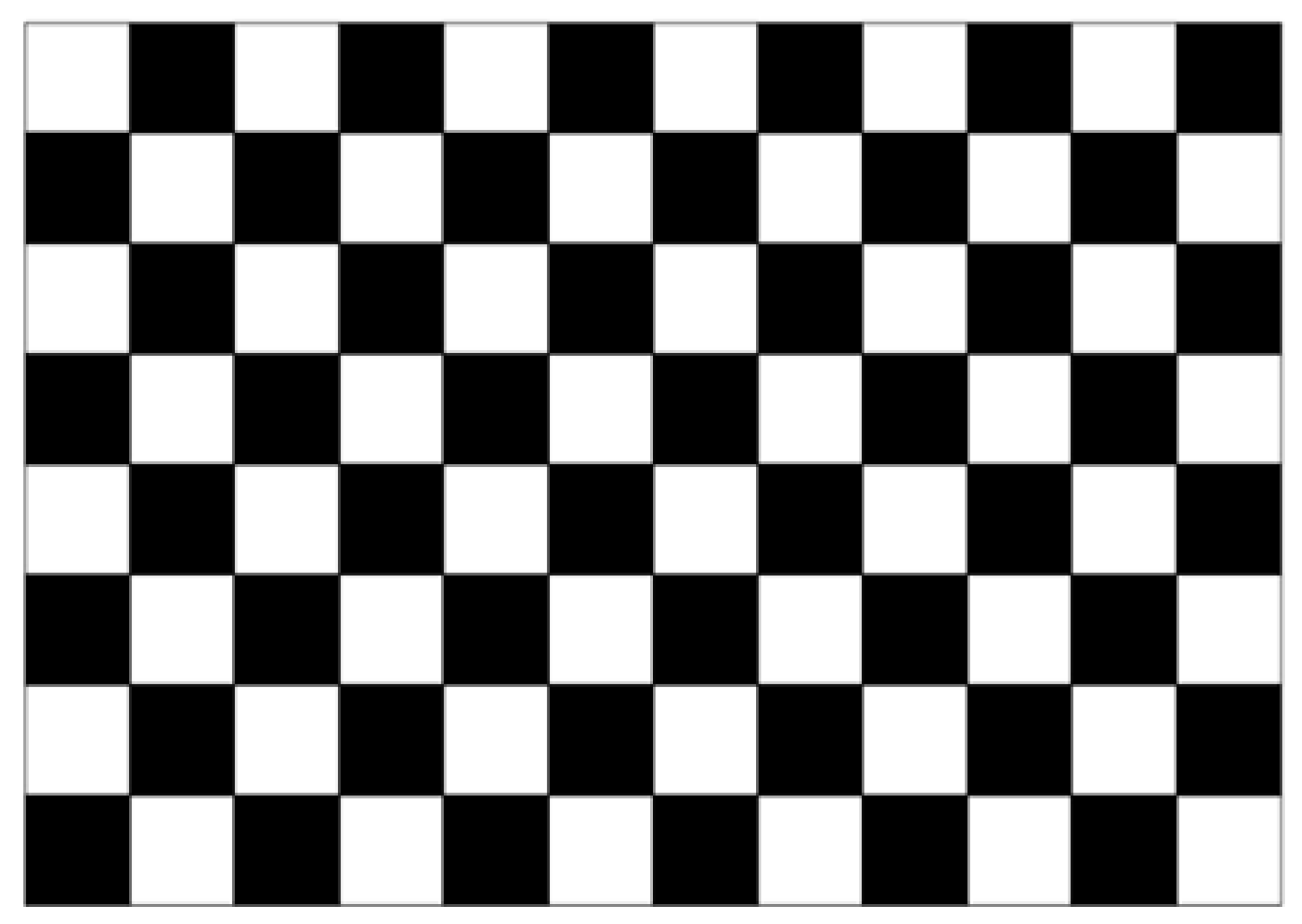
Obtain the template image: position the calibration template before the binocular camera and rotate the calibration template. During each rotation of the calibration template, both cameras simultaneously take pictures. Part of the image obtained with the left camera is shown in Figure 7a.

(2)

Corner coordinate acquisition: considering that the edge part of the checkerboard calibration template is blurred due to the printing quality, the corner points of the edge part are discarded. Four points are manually selected (A, B, C, D). The straight line formed by the 11 corner points closest to the connecting line A and B is the X axis, and the straight line formed by the 7 corner points closest to the connecting line A and D is the Y axis. Then the Harris corner detection algorithm extracts the corner points’ pixel coordinates in the area surrounded by the connecting line between these points, as shown in Figure 7b. The corner points are extracted locally and displayed magnified. Human beings observe the presence of errors, and the corners with errors are corrected artificially.

(3)

Setting up the world coordinate system: for all template images, the corner points in the top left corner are chosen as the reference origin of the world coordinate system. The first row of corner points, both horizontally and vertically, represent the X-axis and Y-axis. All corner points are on the plane, so it is possible to derive all corner points’ coordinates. The coordinates of all corners on the template are consistent in different world coordinate systems.

(4)

Following the aforementioned monocular calibration approach, the individual calibration operations for the left and right cameras are successfully conducted. The resulting calibration parameters for both cameras are provided in

Table 2. Calibration parameters for both cameras.

Parameter	Left Camera	Right Camera
Focal length $[f_x,f_y$]	[911.7311, 912.0249]	[911.5704, 911.5454]
Principal point$\left(u_0,v_0\right)$	(337.9437, 251.4144)	(326.3726, 280.5231)
Non-vertical factor γ	0.4986	−0.3069
Distortion coefficient k	[−0.1062, 0.1594, −5.2870 × 10−4, 8.6057 × 10−4]	[−0.0990, 0.1218, −7.0641 × 10−4, 4.7172 × 10−4]

.

(5)

Using the external parameters for both cameras obtained in the previous step, as presented in

Table 3. External parameters of the binocular camera system.

Parameter	Result
Rotation matrix R	$\left[\begin{array}{ccc}0.9955& -0.0034& -0.0948\\ 0.0032& 1.0000& -0.0019\\ 0.0948& 0.0016& 0.9955\end{array}\right]$
Translation vector T	${\left[\begin{array}{ccc}-83.9391& 0.5500& 2.9898\end{array}\right]}^T$

, the external parameters of the binocular camera system are accessed employing the prescribed solution. Consequently, the calibration process is concluded.

The template’s corner points are reprojected to the corresponding images of both cameras using the calibration parameters of both cameras obtained from the experiment. As illustrated in Figure 8, the projection points’ pixel coordinates are compared with the corners’ actual pixel coordinates in all images. The corresponding re-projection error distribution maps of both cameras are accessed.

Among them, different colors and shapes represent the re-projection errors on the different template images. The coordinate information of each point signifies the disparity between the re-projected points’ pixel coordinates and the actual pixel coordinates in the image.

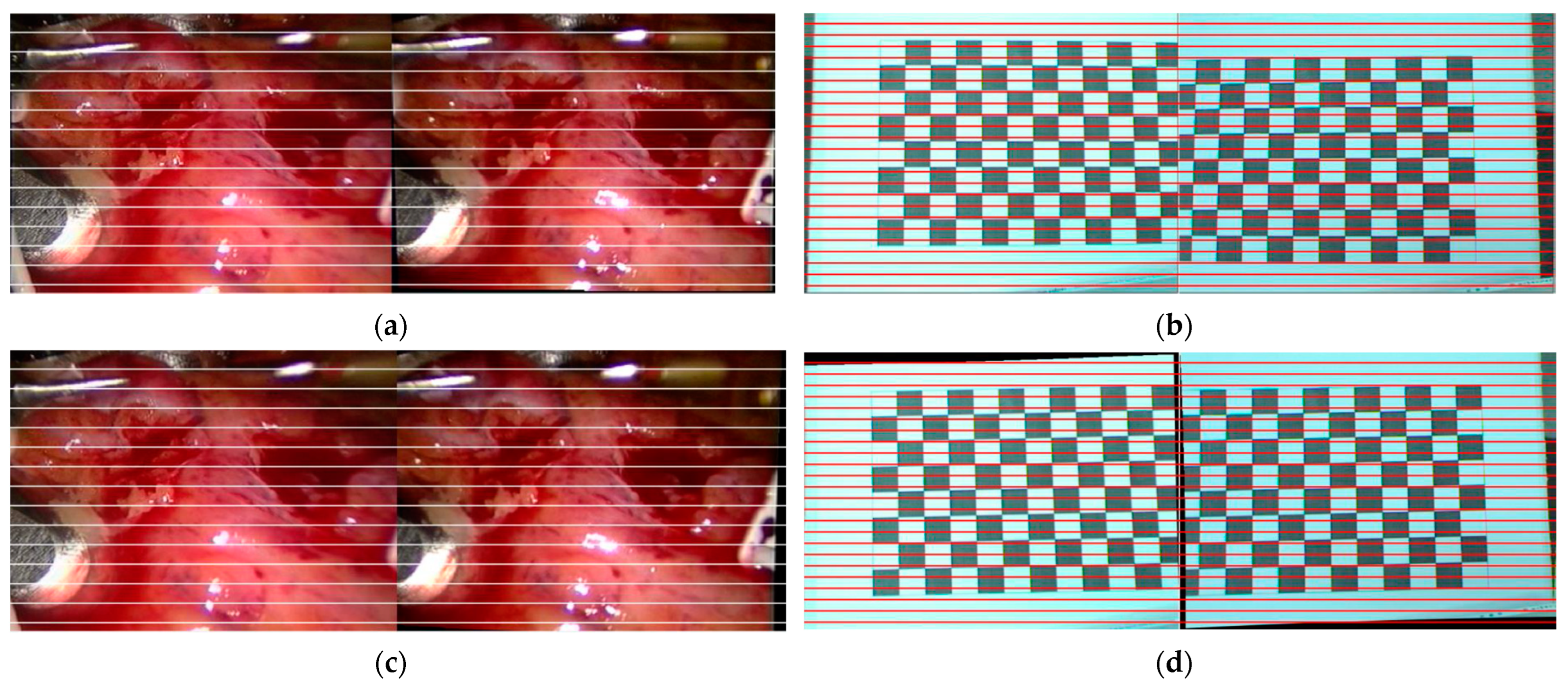
5.2. Binocular Endoscope Image Matching

Figure 9 shows the image comparison before and after correction. It is clear that in Figure 9a, the points in the 3D scene correspond to the non-collinear epipolar lines in the two images. Figure 9b shows a pair of heart images before correction. The polarity lines in the two images do not line up horizontally.

The templates and heart images were corrected using the calibrated binocular camera parameters and the image correction method shown above. The corrected images are shown in Figure 9c,d.

It is obvious that the polarity lines in the two images are not aligned horizontally before correction. The experimental results on real endoscope images demonstrate that after rectification, the image information remains intact while effectively eliminating the vertical disparity. This reduction in vertical disparity significantly narrows down the search range for matching points.

Image registration corrects the vertical disparities caused by the slight variation in the camera’s viewing angles. Removing these vertical disparities enhances the accuracy of depth estimation and reduces artifacts in the reconstructed 3D point cloud. By registering the left and right images accurately, the system can infer the depth information of the different points in the scene more precisely. This results in a more accurate and detailed 3D point cloud reconstruction.

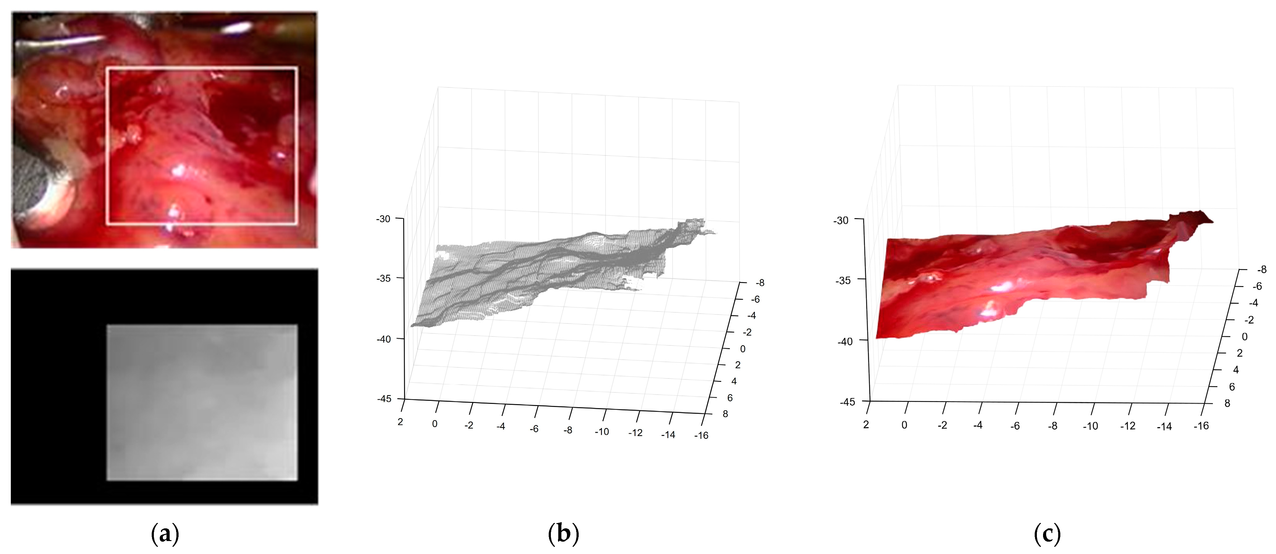
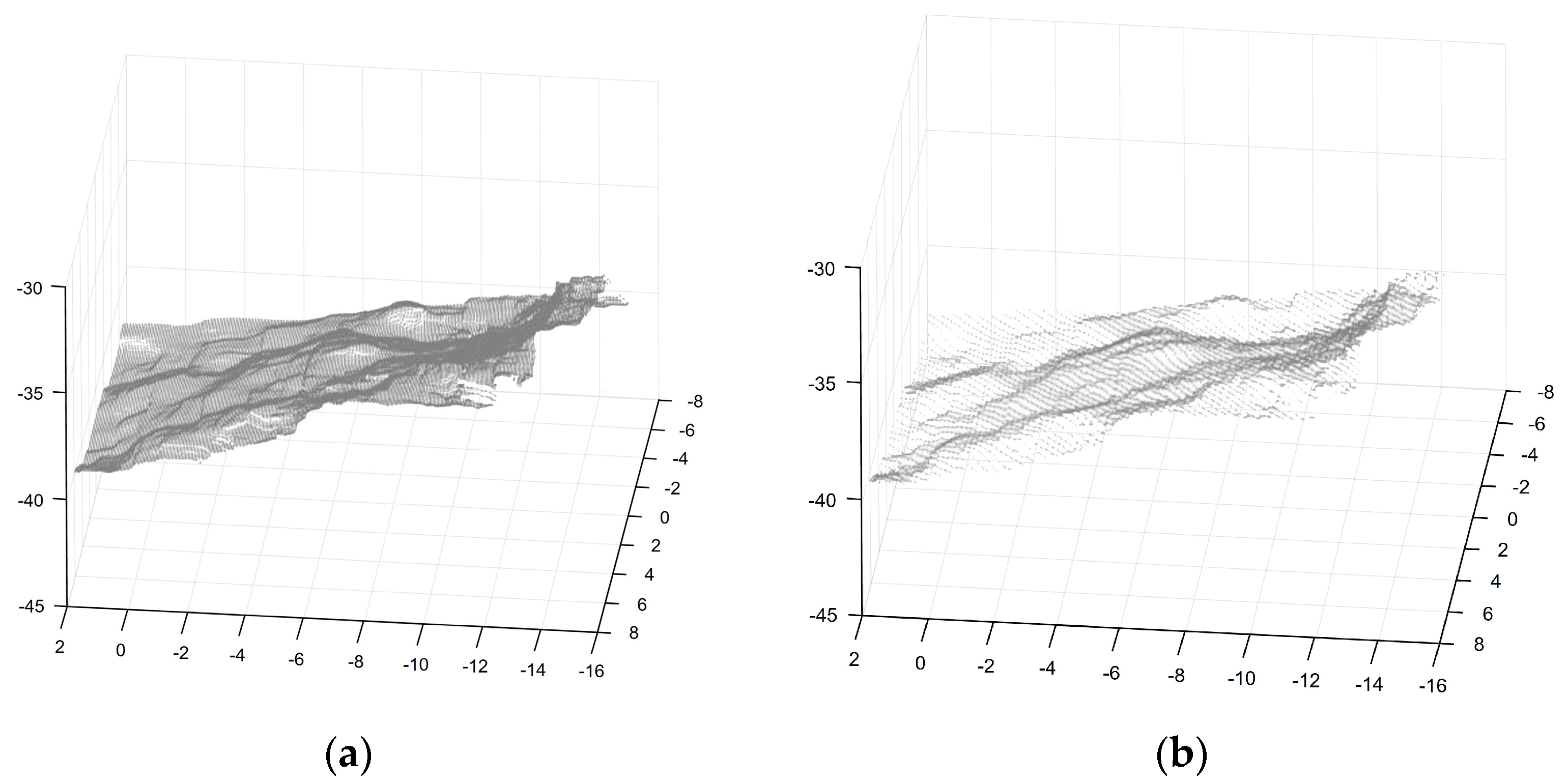
5.3. Three-Dimensional Reconstruction of Cardiac Soft Tissue Surface

First, the 3D point cloud data of the heart soft tissue surface in the target area is obtained by integrating the dense parallax image obtained through a stereo matching algorithm employing a joint similarity measure and adaptive weight [35], as well as the stereo endoscope parameters obtained through the stereo endoscope calibration and the stereo endoscope image correction, combined with the 3D reconstruction method of spatial points, to obtain the three-dimensional point cloud data of the corresponding area of the heart soft tissue surface; measurements are in millimeters (mm). To facilitate observation, the 3D coordinates are rotated under the obtained endoscope coordinate system 180 degrees along its Z-axis and X-axis, respectively, as shown in Figure 10. Figure 10a is the left image of the heart and the corresponding area disparity map. Figure 10b is a three-dimensional point cloud data diagram. Figure 10c shows the three-dimensional point cloud data obtained by adding color information. There are some small bulges or stepped distributions on its corresponding surface, but the surface contour corresponding to its overall transformation trend basically conforms to the rough contour of the surface of the selected block of the interest area.

To facilitate the visual examination of the 3D point cloud data’s surface characteristics, the surface fitting function available in MATLAB is employed. This function enables the direct fitting of the obtained 3D point cloud data to generate a surface representation. Additionally, we extract color information from pixels at 2D image locations in the projection matrix. The extracted color information is associated with the 3D points by storing the extracted color information as attributes of the points in a point cloud data structure. The color information extracted from the selected interest block in the original heart soft tissue image is utilized to enhance the surface visualization. The resulting surface is presented in Figure 10c.

To verify the accuracy of the three-dimensional coordinates of the point cloud obtained, 100 salient image points and their corresponding matching points in the selected interest block are manually marked, and then their corresponding three-dimensional space coordinates are obtained by combining the stereo endoscope parameters and the method in this paper, and they are compared with the 3D coordinates obtained previously. The average absolute deviation is 7.37 (5.92) mm, which is within the allowable range of error, so the obtained 3D point cloud data can be deemed reliable.

The acquired point cloud data are subjected to a filtering process based on the methodology outlined in this study. To prevent excessive smoothing, each parameter is set as $\left[\begin{array}{cc}{\sigma }_s& {\sigma }_d\end{array}\right]=\left[\begin{array}{cc}9& 0.1\end{array}\right]$, and the size of the filtering window is $9\times 9$; that is, it plays a greater role in filtering the points with relatively large changes in their neighborhood so as to remove the deviation points and play a smoothing role in the areas with ladder changes, and perform surface fitting on the filtered and denoised data. Furthermore, down-sampling is performed on the filtered 3D point cloud data. The resulting filtered 3D point cloud and down-sampled 3D point cloud are illustrated in Figure 11.

The result of fitting the reconstructed heart surface with the surface function in MATLAB is shown in Figure 12.

6. Discussion

In the context of binocular stereo vision, the accurate determination of camera parameters is a crucial prerequisite for achieving precise image matching. Once the binocular camera calibration parameters have been obtained, the subsequent step involves the rectification of the stereo image pair. Specifically, this process aims to align the two images so that they exhibit horizontal parallax while eliminating any vertical parallax. This rectification facilitates the feature point matching between the two images, requiring only a horizontal search. Consequently, this approach effectively reduces the search range from two dimensions to a single dimension. To address the aforementioned challenges, this study introduces a binocular camera calibration method and an in-depth image correction technique, followed by a confirmatory experiment. Upon reviewing the results of this experiment, several issues came to light:

A re-projection error occurred during the calibration experiment for the stereoscopic endoscope. This error is believed to stem from two primary sources. Firstly, the utilization of the Harris corner point extraction algorithm for extracting corner point coordinates is prone to some inherent errors. These errors can propagate and affect the subsequent calibration results when incorporating the corner pixel coordinates. Secondly, the maximum likelihood estimation employed in the calibration process refines the obtained parameters, resulting in additional errors. However, as depicted in Figure 8, it is evident that the re-projection errors along the U and V axes corresponding to the left and right endoscopes are concentrated within a range of 0.6 pixels. With a total of 770 corner points comprising 77 corners in each template image across 10 images, the mean Euclidean distance between the re-projected points, which correspond to the actual corner points, was computed. The Euclidean distances associated with the calibration parameters of the two endoscopes were found to be 0.49 (±0.36) and 0.47 (±0.31) pixel units, respectively. Importantly, it is noteworthy that the maximum distance error observed for both the left and right endoscopes remains well within the allowable error range and does not exceed one pixel. Consequently, the calibration results can be deemed highly accurate.

Comparing the images before and after rectification in Figure 9a, it is evident that in the uncorrected images, the epipolar lines of the left and right images are not aligned horizontally. As shown in Figure 9c, after rectification, the image information remains intact, and the vertical disparity values are effectively eliminated. Each corresponding pair of points in both images is horizontally aligned, facilitating the search process during stereo matching. Figure 9b,d in the appendix more intuitively show the difference in template images before and after calibration. To further verify the effectiveness of stereoscopic endoscope image correction, the coordinates of 77 corner points in both template images were acquired. The absolute value of the pixel difference in the vertical direction between the corresponding matching points is counted. The mean absolute value of the pixel difference corresponding to all corners is 0.47 (±0.51) pixels. The maximum deviation is only 0.98 pixels, which is less than a 1-pixel unit, so it is deemed to be within the allowable range of error. This kind of stereoscopic endoscope image correction algorithm is desirable. Simultaneously, this provides additional evidence substantiating the higher precision of the joint calibration algorithm for stereoscopic endoscopes, thereby affirming the feasibility and effectiveness of the calibration algorithm.

The analysis of the corresponding 3D point cloud distribution and its surface fitting results reveals that it provides a rough representation of the heart’s soft tissue surface contour. Nevertheless, notable deviations are observed in the edge regions, with some irregularities resembling ladder-like mutations. These discrepancies stem from the reliance on dense parallax images and stereo endoscope parameters for obtaining the 3D point cloud data. Due to slight variations in the parallax values between the adjacent points in the heart’s soft tissue stereo image, stereo matching introduces deviations. Moreover, the calibration process to determine the stereo endoscope parameters also contributes to inherent inaccuracies. Consequently, cumulative errors give rise to a certain level of deviation between the obtained 3D point cloud and the actual coordinates. The average absolute deviation measures 7.37 (5.92) mm, falling within an acceptable range of error. Thus, the obtained 3D point cloud data are reliable.

Upon comparing the filtered 3D point cloud data with the original counterpart, noticeable observations emerge. Notably, the points positioned on the edges, characterized by significant abrupt changes in the surrounding point cloud data, undergo a certain degree of contraction. Consequently, these points align closer to the 3D coordinates within the denser regions. Consequently, the presence of prominent outliers diminishes, resulting in a smoother appearance in certain areas compared to the original counterpart. Therefore, this filtering operation effectively contributes to the correction of the obtained point cloud data. Simultaneously, the distribution of the down-sampled point cloud data reveals an enhanced ability to accurately depict the heart’s soft tissue surface contour within the targeted area of interest, but its data volume is only 1/10 of the original cloud data; that is, when relying on it for surface reconstruction, it can greatly reduce the time required for triangulation and improve the efficiency of surface reconstruction.

The reconstruction results of the heart soft tissue surface and the results obtained after surface fitting show that there are some uneven phenomena on the reconstructed surface, which is different from the actual heart soft tissue surface. The primary factor contributing to this outcome is the reliance of the 3D point cloud reconstruction on the outcomes of the preceding stages. Its three-dimensional coordinate value is inversely proportional to the corresponding parallax value, and the corresponding heart soft tissue surface is composed of some smooth surfaces; that is, the parallax change between the corresponding adjacent pixel points is very small, so it is inevitable that there will be some errors when obtaining the parallax value, which will lead to this phenomenon in the result of its surface reconstruction. However, from its overall change in trend, it can be seen that the reconstructed cardiac soft tissue surface roughly conforms to the contour of the selected cardiac soft tissue surface corresponding to the interest block area.

7. Conclusions

This study has presented a comprehensive investigation into the calibration and image correction of stereoscopic endoscopes, as well as the 3D surface reconstruction of cardiac soft tissue. The primary objectives of this research were to enhance calibration accuracy, streamline operational procedures, and achieve accurate 3D reconstructions for practical clinical applications. Through a meticulous exploration of internal calibration algorithm parameters and implementation processes, we have successfully developed a novel calibration algorithm that capitalizes on the unique attributes of binocular endoscopes. By integrating principles of monocular camera calibration, our proposed algorithm effectively eliminates vertical disparity while retaining horizontal disparity in stereo images. This not only simplifies the subsequent stereo matching operation but also meets stringent accuracy standards, as evidenced by the robust experimental validation.

Moreover, our investigation into the 3D cardiac soft tissue surface reconstruction method has yielded promising results. The utilization of a stereo endoscope vision system in conjunction with dense parallax images has facilitated accurate 3D coordinate acquisition within the left endoscope coordinate system. The subsequent surface reconstruction process, employing a dual-pass filter and the Delaunay triangulation method, has proven highly effective in generating a detailed and accurate representation of the cardiac soft tissue surface. Our experimental validation demonstrates that the reconstructed 3D spatial points align closely with the manually obtained coordinates, with deviations falling well within acceptable error margins.

However, the study also identified certain limitations, notably the constraint imposed by the necessity for recalibration when performing focus adjustments during endoscope use. This operational restriction presents a practical challenge in clinical settings where focus adjustments are frequently required. As a future research direction, we propose investigating an adaptive calibration approach that leverages initial calibration parameters and automatically adjusts them based on real-time scene characteristics. This avenue of exploration holds the potential for significantly enhancing the usability and practicality of the stereoscopic endoscope system in clinical scenarios.

In conclusion, this study not only contributes novel calibration and image correction algorithms for stereoscopic endoscopes but also presents a robust method for the accurate 3D surface reconstruction of cardiac soft tissue. While some deviations were observed, the results demonstrated the feasibility and effectiveness of the calibration algorithm and provided a reliable basis for cardiac soft tissue surface reconstruction, despite minor irregularities. The results of this study provide theoretical solutions to improve the accuracy and practicality of endoscopic surgery.

References

1. Marr, D.; Poggio, T.; Hildreth, E.C.; Grimson, W.E.L. A computational theory of human stereo vision. In From the Retina to the Neocortex: Selected Papers of David Marr; Vaina, L., Ed.; Birkhäuser Boston: Boston, MA, USA, 1991; pp. 263–295. [Google Scholar] [CrossRef]
2. Ji, Y.; Li, Y.; Sun, X.; Yan, S.; Guo, N. Stereo matching algorithm based on binocular vision. In Proceedings of the 2020 7th International Forum on Electrical Engineering and Automation (IFEEA), Hefei, China, 25–27 September 2020; pp. 843–847. [Google Scholar] [CrossRef]
3. Lu, S.; Yang, J.; Yang, B.; Yin, Z.; Liu, M.; Yin, L.; Zheng, W. Analysis and Design of Surgical Instrument Localization Algorithm. Comput. Model. Eng. Sci. 2023, 137, 669–685. [Google Scholar] [CrossRef]
4. Zhang, Y.-J. Camera calibration. In 3-D Computer Vision: Principles, Algorithms and Applications; Springer: Berlin/Heidelberg, Germany, 2023; pp. 37–65. [Google Scholar] [CrossRef]
5. Tang, Y.; Liu, S.; Deng, Y.; Zhang, Y.; Yin, L.; Zheng, W. An improved method for soft tissue modeling. Biomed. Signal Process. Control. 2021, 65, 102367. [Google Scholar] [CrossRef]
6. Dang, W.; Xiang, L.; Liu, S.; Yang, B.; Liu, M.; Yin, Z.; Yin, L.; Zheng, W. A Feature Matching Method based on the Convolutional Neural Network. J. Imaging Sci. Technol. 2023, 67, 1–11. [Google Scholar] [CrossRef]
7. Lu, S.; Liu, S.; Hou, P.; Yang, B.; Liu, M.; Yin, L.; Zheng, W. Soft Tissue Feature Tracking Based on DeepMatching Network. CMES Comput. Model. Eng. Sci. 2023, 136, 363–379. [Google Scholar]
8. Han, R.; Yan, H.; Ma, L. Research on 3D Reconstruction methods Based on Binocular Structured Light Vision. J. Phys. Conf. Ser. 2021, 1744, 032002. [Google Scholar] [CrossRef]
9. Liu, X.; Zheng, W.; Mou, Y.; Li, Y.; Yin, L. Microscopic 3D reconstruction based on point cloud data generated using defocused images. Meas. Control. 2021, 54, 1309–1318. [Google Scholar] [CrossRef]
10. Zhu, J.; Lyu, L.; Xu, Y.; Liang, H.; Zhang, X.; Ding, H.; Wu, Z. Intelligent Soft Surgical Robots for Next-Generation Minimally Invasive Surgery. Adv. Intell. Syst. 2021, 3, 2100011. [Google Scholar] [CrossRef]
11. Hardner, M.; Docea, R.; Schneider, D. Guided Calibration of Medical Stereo Endoscopes. Int. Arch. Photogramm. Remote Sens. Spatial Inf. Sci. 2022, XLIII-B2-2022, 679–686. [Google Scholar] [CrossRef]
12. Edwards, P.J.E.; Psychogyios, D.; Speidel, S.; Maier-Hein, L.; Stoyanov, D. SERV-CT: A disparity dataset from cone-beam CT for validation of endoscopic 3D reconstruction. Med. Image Anal. 2022, 76, 102302. [Google Scholar] [CrossRef]
13. Huo, J.; Zhou, C.; Yuan, B.; Yang, Q.; Wang, L. Real-Time Dense Reconstruction with Binocular Endoscopy Based on StereoNet and ORB-SLAM. Sensors 2023, 23, 2074. [Google Scholar] [CrossRef]
14. Davies, M.; Stuart, M.B.; Hobbs, M.J.; McGonigle, A.J.; Willmott, J.R. Image correction and In situ spectral calibration for low-cost, smartphone hyperspectral imaging. Remote Sens. 2022, 14, 1152. [Google Scholar] [CrossRef]
15. Suganyadevi, S.; Seethalakshmi, V.; Balasamy, K. A review on deep learning in medical image analysis. Int. J. Multimed. Inf. Retr. 2022, 11, 19–38. [Google Scholar] [CrossRef] [PubMed]
16. Zhang, Z. A flexible new technique for camera calibration. IEEE Trans. Pattern Anal. Mach. Intell. 2000, 22, 1330–1334. [Google Scholar] [CrossRef]
17. Lü, X.; Meng, L.; Long, L.; Wang, P. Comprehensive improvement of camera calibration based on mutation particle swarm optimization. Measurement 2022, 187, 110303. [Google Scholar] [CrossRef]
18. Miyawaki, T.; Endo, K. Optical path length self-calibration method based on form measured surface data. Precis. Eng. 2022, 77, 360–364. [Google Scholar] [CrossRef]
19. Barone, F.; Marrazzo, M.; Oton, C.J. Camera calibration with weighted direct linear transformation and anisotropic uncertainties of image control points. Sensors 2020, 20, 1175. [Google Scholar] [CrossRef]
20. Kwon, Y.-H. A non-linear camera calibration algorithm: Direct Solution Method. In Proceedings of the ISBS-Conference Proceedings Archive, Beijing, China, 22–27 August 2005; p. 142. [Google Scholar]
21. Gee, T.; Delmas, P.; Stones-Havas, N.; Sinclair, C.; Mark, W.V.D.; Li, W.; Friedrich, H.; Gimel’farb, G. Tsai camera calibration enhanced. In Proceedings of the 2015 14th IAPR International Conference on Machine Vision Applications (MVA), Tokyo, Japan, 18–22 May 2015; pp. 435–438. [Google Scholar] [CrossRef]
22. Kumar, A.; Wang, Y.-Y.; Wu, C.-J.; Liu, K.-C.; Wu, H.-S. Stereoscopic visualization of laparoscope image using depth information from 3D model. Comput. Methods Programs Biomed. 2014, 113, 862–868. [Google Scholar] [CrossRef]
23. Luo, H.; Yin, D.; Zhang, S.; Xiao, D.; He, B.; Meng, F.; Zhang, Y.; Cai, W.; He, S.; Zhang, W.; et al. Augmented reality navigation for liver resection with a stereoscopic laparoscope. Comput. Methods Programs Biomed. 2020, 187, 105099. [Google Scholar] [CrossRef]
24. Wang, Y.; Long, Y.; Fan, S.H.; Dou, Q. Neural Rendering for Stereo 3D Reconstruction of Deformable Tissues in Robotic Surgery. In Proceedings of the Medical Image Computing and Computer Assisted Intervention—MICCAI 2022, Singapore, 18–22 September 2022; pp. 431–441. [Google Scholar] [CrossRef]
25. Zicheng, L.; He, Y.; Hongya, W.; Liang, C.; Quan, Z. Research Progress in 3D-reconstruction Based Imaging Analysis in Partial Solid Pulmonary Nodule. Chin. J. Lung Cancer 2022, 25, 124–129. [Google Scholar]
26. Wu, Z.; Guo, W.; Chen, Z.; Wang, H.; Li, X.; Zhang, Q. Three-dimensional shape and deformation measurement on complex structure parts. Sci. Rep. 2022, 12, 7760. [Google Scholar] [CrossRef]
27. Zenteno, O.; Trinh, D.-H.; Treuillet, S.; Lucas, Y.; Bazin, T.; Lamarque, D.; Daul, C. Optical biopsy mapping on endoscopic image mosaics with a marker-free probe. Comput. Biol. Med. 2022, 143, 105234. [Google Scholar] [CrossRef] [PubMed]
28. Bao, J.; Jing, J.; Zhang, W.; Liu, C.; Gao, T. A corner detection method based on adaptive multi-directional anisotropic diffusion. Multimed. Tools Appl. 2022, 81, 28729–28754. [Google Scholar] [CrossRef]
29. Han, Z.; Zhang, L. Modeling and Calibration of a Galvanometer-Camera Imaging System. IEEE Trans. Instrum. Meas. 2022, 71, 1–9. [Google Scholar] [CrossRef]
30. Xuechun, W.; Liang, W.; Fuqing, D. Calibration for light field cameras based on fixed point constraint of spatial plane homography. Opt. Express 2022, 30, 24968–24983. [Google Scholar] [CrossRef]
31. Lang, J.; Mao, J.; Liang, R. Non-horizontal target measurement method based on monocular vision. Syst. Sci. Control. Eng. 2022, 10, 443–458. [Google Scholar] [CrossRef]
32. Wang, D.; Hu, L.-L. Improved Feature Stereo Matching Method Based on Binocular Vision. Acta Electonica Sin. 2022, 50, 157. [Google Scholar] [CrossRef]
33. Mehedi, I.M.; Rao, K.P.; Alotaibi, F.M.; Alkanfery, H.M. Intelligent Wireless Capsule Endoscopy for the Diagnosis of Gastrointestinal Diseases. Diagnostics 2023, 13, 1445. [Google Scholar] [CrossRef]
34. Boese, A.; Wex, C.; Croner, R.; Liehr, U.B.; Wendler, J.J.; Weigt, J.; Walles, T.; Vorwerk, U.; Lohmann, C.H.; Friebe, M.; et al. Endoscopic Imaging Technology Today. Diagnostics 2022, 12, 1262. [Google Scholar] [CrossRef]
35. Xi, L.; Zhao, Y.; Chen, L.; Gao, Q.H.; Tang, W.; Wan, T.R.; Xue, T. Recovering dense 3D point clouds from single endoscopic image. Comput. Methods Programs Biomed. 2021, 205, 106077. [Google Scholar] [CrossRef]
Figure 1. Checkerboard template.
Electronics 12 03799 g001
Figure 2. Endoscopic image of the heart.
Electronics 12 03799 g002
Figure 3. The epipolar geometric relationship before correction.
Electronics 12 03799 g003
Figure 4. Schematic diagram of the first rotation.
Electronics 12 03799 g004
Figure 5. Schematic diagram of the second rotation.
Electronics 12 03799 g005
Figure 6. Correction schematic diagram.
Electronics 12 03799 g006
Figure 7. Template image acquisition and collection. (a) Partial template image of the left camera; (b) corner extraction of the template image.
Electronics 12 03799 g007
Figure 8. Projection error distribution. (a) Left camera; (b) right camera.
Electronics 12 03799 g008
Figure 9. Image comparison before and after correction. (a) Cardiac image pairs before the correction; (b) template image pair before the correction; (c) corrected heart image pairs; (d) template image pairs after correction.
Electronics 12 03799 g009
Figure 10. Point cloud 3D reconstruction data. (a) Left cardiac image and parallax map of corresponding regions; (b) 3D point cloud data; (c) point cloud data direct surface fitting results.
Electronics 12 03799 g010
Figure 11. Three-dimensional point cloud after filtering and 3D point cloud after down-sampling. (a) Three-dimensional point cloud after filtering; (b) 3D point cloud after down-sampling.
Electronics 12 03799 g011
Figure 12. The reconstructed heart surface and its surface fitting results. (a) The reconstructed cardiac surface; (b) surface fitting results.
Electronics 12 03799 g012