Improving Monocular Depth Estimation with Learned Perceptual Image Patch Similarity-Based Image Reconstruction and Left–Right Difference Image Constraints

Abstract

This paper introduces a novel approach for self-supervised monocular depth estimation. The model is trained on stereo–image (left–right pair) data and incorporates carefully designed perceptual image quality assessment-based loss functions for image reconstruction and left–right image difference. The fidelity of the reconstructed images, obtained by warping the input images using the predicted disparity maps, significantly influences the accuracy of depth estimation in self-supervised monocular depth networks. The suggested LPIPS (Learned Perceptual Image Patch Similarity)-based evaluation of image reconstruction accurately emulates human perceptual mechanisms to quantify the quality of reconstructed images, serving as an image reconstruction loss. Consequently, it facilitates the gradual convergence of the reconstructed images toward a greater similarity with the target images during the training process. Stereo–image pair often exhibits slight discrepancies in brightness, contrast, color, and camera angle due to factors like lighting conditions and camera calibration inaccuracies. These factors limit the improvement of image reconstruction quality. To address this, the left–right difference image loss is introduced, aimed at aligning the disparities between the actual left–right image pair and the reconstructed left–right image pair. Due to the tendency of distant pixel values to approach zero in the difference images derived from the left and right source images of stereo pairs, this loss progressively steers the distant pixel values of the reconstructed difference images toward a convergence with zero. Hence, the use of this loss has demonstrated its efficacy in mitigating distortions in distant regions while enhancing overall performance. The primary objective of this study is to introduce and validate the effectiveness of LPIPS-based image reconstruction and left–right difference image losses in the context of monocular depth estimation. To this end, the proposed loss functions have been seamlessly integrated into a straightforward single-task stereo–image learning framework, incorporating simple hyperparameters. Notably, our approach achieves superior results compared to other state-of-the-art methods, even those adopting more intricate hybrid data and multi-task learning strategies.

1. Introduction

Deep learning-based monocular depth estimation methods have gained significant attention due to their ability to estimate depth maps from single images without relying on expensive external sensors such as RGB-D cameras and LiDAR [1,2,3]. The capability of end-to-end depth estimation from single images has profound implications for various fields, including robotics, autonomous driving, virtual reality, augmented reality, and medical imaging. Deep learning-based monocular depth estimation can be broadly categorized into supervised learning, self-supervised learning, and semi-supervised learning [2,4]. While various supervised learning approaches achieve high-ranking results, they all require a substantial amount of labeled datasets, which is expensive to obtain using RGB-D cameras or LiDAR sensors. On the other hand, self-supervised learning is a more cost-effective approach but requires additional well-designed constraints to maintain geometric consistency for stereo–image data learning and photometric consistency for video sequence learning. Semi-supervised learning combines supervised and self-supervised approaches by utilizing a small amount of labeled dataset and the remaining unlabeled dataset.

This study introduces an innovative technique for self-supervised monocular depth estimation. The proposed approach integrates a loss based on a perceptual image quality assessment model, with a specific focus on enhancing image reconstruction and addressing left–right image differences during model training. The proposed loss plays a pivotal role in the training process, leading to refined precision in monocular depth estimation. Within this framework, the neural network undergoes training using only paired stereo–images from the provided dataset, enabling the prediction of depth maps from a solitary image without reliance on ground-truth data. The primary objective involves minimizing the loss in image reconstruction, ensuring a close correspondence between the image under reconstruction and the respective reference image captured from an alternative viewpoint within the dataset. Through the minimization of this loss, the model strives to establish a notable resemblance connecting the reconstructed and referenced images. This enhancement serves to bolster the precision of monocular depth estimation, a key aspect of the evaluation. Throughout the training process, the network learns to predict the disparity map, which represents a pixel-wise inverse depth map and is essential for reconstructing an image from another viewpoint. As the training progresses, the quality of the reconstructed images improves gradually, leading to an enhanced accuracy of the disparity map.

The image reconstruction process plays a crucial role in this approach, as the quality of the reconstructed images affects the precision of the predicted disparity maps. Therefore, a well-designed image reconstruction loss is essential. This loss serves as a guiding mechanism during training, facilitating effective image reconstruction and enabling the derivation of an accurate disparity map for the source image. Previous works in the field have commonly used L1- and SSIM-based [5] image reconstruction loss, as proposed by [3]. While it has shown effectiveness, it may have limitations, especially in challenging areas of an image, such as low-texture regions, homogeneous regions, and distant areas like the sky, forest, and road. In such cases, where feature point extraction becomes difficult, the existing losses may lack sufficient accuracy and robustness. Recently, learning-based perceptual image quality assessment models like PieAPP (Perceptual Image-Error Assessment through Pairwise Preference) [6] and LPIPS (Learned Perceptual Image Patch Similarity) [7] have shown greater effectiveness compared to traditional computer vision-based algorithms in assessing image quality, especially in images with challenging areas. In this study, we departed from the conventional use of SSIM and instead integrated a pre-trained LPIPS model into our image reconstruction loss. Unlike SSIM, LPIPS is a perceptual image quality assessment algorithm trained to align with human perception based on extensive human perceptual judgments. By incorporating LPIPS, our aim is to enhance the perceptual similarity between the reconstructed and the target images, thus reducing artifacts even in challenging areas of the reconstructed images. This approach utilizes the power of human perception to improve the overall quality of the reconstructed images.

Although the integration of LPIPS-based image reconstruction loss shows an enhanced performance compared to the conventional SSIM-based loss in experiments, it still faces challenges in effectively addressing distortions caused by variations between the left and right reference images. Inherent factors such as lighting conditions and camera calibration errors lead to unavoidable slight variations in brightness, contrast, color, and camera angle within pairs of stereo–image. These variations constrain the enhancement of reconstruction quality.

In response to this challenge, we introduce an innovative loss referred to as the “left–right difference image loss.” Utilizing an auto-encoder network architecture, our proposed model primarily reconstructs both the left and right images. These reconstructed images are also utilized to generate two distinct difference images, each serving a specific purpose: one originates from the reconstructed left and right image pair, while the other is derived from the corresponding target pair. The left–right difference image loss combines L1 loss and LPIPS-based loss. This composite loss facilitates the alignment between the difference images of the reconstructed pairs and the corresponding ones from the target pairs. Throughout the training process, it consistently aligns the pixel values of the reconstructed difference images with those of the target difference images. Considering that pixel values in distant regions of a reference image pair generally display minor disparities, leading to minimal visual divergence, the proposed loss steers these remote pixel values within the reconstructed difference image toward a convergence with zero. As a result, the incorporation of this loss effectively mitigates distortions arising from variations between the left and right reference images, while also addressing distortions present in remote regions.

To showcase the efficacy of our proposed losses, we integrated them into a ResNet50-based network [8]. The model was trained using stereo–image pairs from the KITTI 2015 dataset [9] to generate depth maps for $640\times 192$ images. Extensive experimentation demonstrated the notable improvement of our approach. Remarkably, our method outperforms several state-of-the-art studies employing more complex approaches, such as hybrid data learning of stereo–image and video sequence, as well as multi-task learning of depth and semantic segmentation. These results highlight the effectiveness and robustness of our proposed approach in the domain of self-supervised monocular depth estimation.

2. Related Work

2.1. Monocular Depth Estimation with Stereo–Image Data Learning

Active research has been conducted in the field of supervised monocular depth estimation neural networks, which learn using datasets that include depth ground-truth data since Eigen et al. [1] proposed a technique for inferring depth maps from monocular color images using deep learning [10,11,12]. However, the continuous development of supervised monocular depth estimation faces challenges in terms of the time and cost required to create large-scale datasets with depth maps for training [2,3,4]. To address this issue, research on self-supervised depth estimation networks that do not rely on ground-truth depth maps has emerged. These networks use unlabeled stereo–image and/or monocular video sequence datasets and utilize geometric and photometric constraints between frames as supervisory signals during the learning process [2,4]. Garg et al. [13] introduced a self-supervised framework for monocular depth prediction that centers on learning from stereo–images without necessitating a pre-training phase or annotated depth ground truth. They adopt the L2 loss between the reconstructed and target images as a straightforward image reconstruction loss. However, this approach leads to the generation of blurry images, as it tends to converge to a stable value without achieving precise pixel-level values. Subsequent research introduced a more sophisticated image reconstruction loss, combining L1 loss and SSIM-based [5] loss proposed by Godard et al. [3]. They also proposed a disparity smoothness loss and a left–right consistency loss. SSIM-based loss has since been widely employed in self-supervised depth estimation networks, including in works by Pillai et al. [14,15,16]. Park et al. [17] proposed a self-supervised depth prediction model using GMSD [18], a conventional IQA algorithm, as the image reconstruction loss in a symmetric GAN [19] structure. They demonstrated that the GMSD-based loss could effectively improve the accuracy of monocular depth estimation. Park et al. [20] also proposed a self-supervised model for stereo–image learning. They introduced a specialized image reconstruction loss based on PieAPP [6].

2.2. Monocular Depth Estimation with Video Sequence Data Learning

Zhou et al. [21] introduced a self-supervised model for depth estimation, focusing on learning from monocular video sequences. The approach involves the joint training of two networks on unlabeled video sequences: one dedicated to depth prediction and the other to estimating camera poses. L1 loss is employed for image synthesis during this process. Mahjourian et al. [22] presented a novel self-supervised method for learning depth and ego-motion from successive video frames. Yin et al. [23] proposed GeoNet, a comprehensive training paradigm that employs three networks for monocular depth, optical flow, and ego-motion estimation from consecutive video frames. This is achieved using a robust image similarity measurement based on SSIM. Wang et al. [24] suggested an enhancement by integrating the direct visual odometry (DVO) [25] pose predictor into a self-supervised video sequence learning model, replacing the PoseCNN. This revised model employs a linear combination of L1 loss and SSIM for image reconstruction loss. EPC++ network [26] was proposed to jointly train three networks based on video sequences, for depth prediction (DepthNet), camera motion (MotionNet), and optical flow (OptFlowNet). Li et al. [27] presented a method for jointly training depth, ego-motion, and a dense 3D translation field of objects relative to the scene, using an SSIM-based image reconstruction loss. Xiong et al. [28] proposed using robust geometric losses to align the scales of two reconstructed depth maps estimated from adjacent video frames, enforcing forward–backward relative pose consistency, and formulating scale-consistent geometric constraints.

2.3. Monocular Depth Estimation with Hybrid Data and Multi-Task Learning

Godard et al. [15] extended their stereo–image learning model to propose a self-supervised monocular depth estimation framework that encompasses learning from consecutive video frames. Their model incorporated a minimal reprojection loss to address occlusion, employed a full-resolution multi-scale sampling technique to manage visual artifacts, and integrated a straightforward auto-masking approach to exclude pixels exhibiting consistent appearances across frames. Rottmann et al. [16] proposed a self-supervised multi-task learning model that jointly trained semantic segmentation and depth estimation. They used both stereo–image dataset and video sequence dataset for training and designed their image reconstruction loss based on SSIM with whole-image input. SGDepth [29] also adopted multi-task learning for semantic segmentation and depth estimation, with a focus on dynamic-class objects such as moving cars and pedestrians. They trained their network only on video sequence data. Similar multi-task learning approaches based on monocular video sequence data learning were suggested in [30,31]. Guizilini et al. [32] also proposed a multi-task learning self-supervised monocular depth estimation model with a semantic segmentation network to guide geometric representation learning. They used a two-stage training process to automatically detect the presence of a common bias on dynamic objects. SceneNet [33] proposed a stereo–image multi-task learning-based cross-modal network model that incorporated semantic information to guide disparity smoothness.

3. Proposed Model

This section presents a detailed description of the network architecture employed in the proposed self-supervised monocular depth estimation model. Additionally, it provides a comprehensive explanation of the training losses incorporated into the model’s framework.

3.1. Depth Estimation Network Architecture

The proposed network architecture employs a self-supervised approach for monocular depth estimation, utilizing stereo–image data for training. As illustrated in Figure 1, the overall network architecture aims to minimize various losses for multi-scale disparity maps, including image reconstruction loss, left–right disparity consistency loss, disparity smoothness loss, and left–right difference image loss. These losses contribute to the effective training and optimization of the network, facilitating an improved depth estimation performance. The network learns how to estimate disparity, i.e., inverse depth values for reconstructing a different view image ${\widehat{I}}_r$ (right) from a given input image $I_l$ (left) in a self-supervised manner by training on stereo–image pairs. The depth p can be determined using the formula $p=(b\times f)/d$, wherein b denotes the baseline distance between two cameras, f represents the camera’s focal length, and d stands for the disparity map. Upon completion of the learning process, the network acquires the capability to generate a precise reconstruction of a distinct view image by leveraging the estimated disparity map. Consequently, it becomes proficient in estimating the disparity at a pixel-wise level within a single-source image. This means that the network can effectively infer the relative distances of objects in the scene based on their corresponding pixel disparities, enabling an accurate estimation of depth information. Our approach is inspired by Godard et al. [2] and we deploy a simple ResNet50-based auto-encoder that only trains stereo–image data of the KITTI dataset.

In the decoder component of our network, we integrate six up-convolution layers that facilitate upsampling. This is achieved through bilinear interpolation, with a consistent scale factor of two applied in each successive layer. This procedure generates four pairs of left–right disparity maps, each of varying sizes. The right disparity map ($d_r$) is employed to synthesize a reconstructed right image (${\widehat{I}}_r$) from a source left image ($I_l$) using the warping process denoted as $w_{+}$. Similarly, the left disparity map ($d_l$) is utilized to synthesize a reconstructed left image (${\widehat{I}}_l$) from a source right image ($I_r$) simultaneously, accomplished through the warping process represented as $w_{-}$.

By utilizing these disparity maps and the warping processes, the network simultaneously synthesizes both left and right images while maintaining consistency between the disparities of the two. Since the network is trained without access to depth ground-truth data, it determines optimal parameters by evaluating the similarity between the reconstructed and target images. This similarity is quantified as the image reconstruction loss. Essentially, a strong resemblance between the reconstructed and target images indicates accurate disparity predictions by the network.

To address this, we take into consideration the relative performance of image quality assessment (IQA) models. Deep learning-based perceptual IQA models have consistently demonstrated superiority over conventional computer vision-based models across various metrics. Therefore, rather than employing the commonly used combination of SSIM and L1 loss as the image reconstruction loss in previous studies, we opt for a combination of a pre-trained LPIPS model ($L^{lpips}$) and L1 loss ($L^{L1}$) for this particular purpose.

Despite the inclusion of the left–right disparity consistency loss, as suggested in [3], its effectiveness in addressing concurrent distortions present in both the left and right disparity maps is found to be insufficient. This limitation arises from the aforementioned variations and the scarcity of feature points, particularly in challenging regions. To overcome this, the integration of the left–right difference image loss ($L^{diff}$) within our model provides a valuable mechanism to directly minimize the difference between the reconstructed difference image and the source difference image. This approach effectively mitigates the distortions, resulting in improved accuracy and fidelity in the reconstructed images. Furthermore, this loss plays a crucial role in effectively enhancing the quality of reconstruction, especially in distant regions, by gradually guiding the distant pixel values of the reconstructed difference images toward convergence with zero.

3.2. Training Loss

Image Reconstruction Loss: Training of the monocular depth estimation network aims to generate a disparity map that accurately synthesizes a given input image to resemble a target image. To achieve this, an image reconstruction loss is employed to measure the numerical discrepancy between the reconstructed and target images. By minimizing this loss, the network finds parameters to enhance the overall quality of the synthesized images and optimize its depth estimation capabilities. In the proposed network, we have opted to utilize a pre-trained LPIPS [7] model as a component of our image reconstruction loss ($L^{lpips}$). This choice is motivated by the algorithm’s ability to effectively address distortions encountered in challenging regions of the reconstructed images. By leveraging the capabilities of LPIPS, we can better evaluate and minimize the perceptual differences between the two images, leading to an improved image reconstruction quality. Additionally, we integrate L1 loss ($L^{L1}$) to enhance the quality of the reconstructed images. This is achieved by minimizing the absolute pixel-wise disparity between the corresponding reconstructed and target images. As a result, the image reconstruction loss, labeled as $L^{rec}$, can be formulated as follows:

$${\widehat{I}}_r=w_{+}(I_l,d_r)$$

(1)

$${\widehat{I}}_l=w_{-}(I_r,d_l)$$

(2)

$$L_r^{lpips}=\sum lpips(I_r,{\widehat{I}}_r)$$

(3)

$$L_l^{lpips}=\sum lpips(I_l,{\widehat{I}}_l)$$

(4)

$$L^{lpips}=L_r^{lpips}+L_l^{lpips}$$

(5)

$$L_r^{L1}=\sum \Vert I_r-{\widehat{I}}_r\Vert$$

(6)

$$L_l^{L1}=\sum \Vert I_l-{\widehat{I}}_l\Vert$$

(7)

$$L^{L1}=L_r^{L1}+L_l^{L1}$$

(8)

$$L^{rec}=L^{lpips}+L^{L1}$$

(9)

Disparity Smoothness Loss: As in [3,15], we include an edge-aware smoothness loss ($L^{smooth}$) to promote local depth consistency in edge boundary regions. The objective of this loss is to encourage adjacent pixels in the edge region to have similar depth values, based on the assumption that they likely belong to the same object or similar locations. This principle is employed for both the left and right disparity maps generated from the input. As a result, corresponding smoothness losses ($L_l^{smooth}$ and $L_r^{smooth}$) are formulated. The disparity smoothness loss is defined as follows:

$$L_r^{smooth}=\sum |{\partial }_x{d}_r^{*}|e^{-|{\partial }_x{I}_r|}+\left|{\partial }_y{d}_r^{*}\right|e^{-|{\partial }_y{I}_r|}$$

(10)

$$L_l^{smooth}=\sum |{\partial }_x{d}_l^{*}|e^{-|{\partial }_x{I}_l|}+\left|{\partial }_y{d}_l^{*}\right|e^{-|{\partial }_y{I}_l|}$$

(11)

$$L^{smooth}=L_r^{smooth}+L_l^{smooth}$$

(12)

$d^{*}=d/\overline{d}$ represents the mean-normalized disparity obtained from [24]. The symbol $\partial d$ corresponds to the gradient of the disparity, while $\partial I$ represents the gradient of the image. The gradient is calculated for each axis in the given disparity map using partial derivatives with respect to the x and y axes, as specified by the equation. Due to the steep gradient variations near the edges, a weight-based exponential scaling is applied to reduce the scale.

Left–Right Disparity Consistency Loss: Furthermore, we incorporated the left–right consistency loss proposed by Godard et al. [3] into our model. In essence, it evaluates the difference between the left disparity map and the projected right disparity map, and vice versa. Therefore, it involves comparing the left-to-right disparity map ($d_{l2r}$), obtained through the warping process $w_{+}$, with the right disparity map ($d_r$), as well as the right-to-left disparity map ($d_{r2l}$), obtained through the warping process $w_{-}$, with the left disparity map ($d_l$). This process is designed to ensure alignment and consistency between left and right disparity maps, contributing to the overall accuracy and quality of the depth estimation. This loss is defined as follows:

$$d_{l2r}=w_{+}(d_l,d_r)$$

(13)

$$d_{r2l}=w_{-}(d_r,d_l)$$

(14)

$$L_r^{con}=\sum \Vert d_{l2r}-d_r\Vert$$

(15)

$$L_l^{con}=\sum \Vert d_{r2l}-d_l\Vert$$

(16)

$$L^{con}=L_r^{con}+L_l^{con}.$$

(17)

Left–Right Difference Image Loss: Here, the term “difference image” means simply subtracting the right image from the left image, providing another hint as to how much a particular pixel has to move during the reconstruction process. The left–right difference image loss serves a crucial role in guiding the pixel values of the reconstructed difference images to closely resemble the corresponding values in the target difference images, which complements and enhances the image reconstruction loss by further enforcing consistency. To ensure consistency with the proposed image reconstruction loss, we formulated the left and right difference image loss by combining L1 loss and LPIPS-based loss. The left–right difference image loss, denoted as $L^{diff}$, is defined as follows:

$$L_{l1}^{diff}=\sum \Vert (I_l-I_r)-({\widehat{I}}_l-{\widehat{I}}_r)\Vert$$

(18)

$$L_{lpips}^{diff}=\sum lpips((I_l-I_r),({\widehat{I}}_l-{\widehat{I}}_r))$$

(19)

$$L^{diff}=L_{l1}^{diff}+L_{lpips}^{diff}$$

(20)

Total training loss: The main purpose of this study is to prove the effect of the proposed LPIPS-based image reconstruction loss and left–right difference image loss, so each loss function is designed to contribute to the total loss with the same weight. Thus, the total training loss, obtained by simply combining all the proposed losses, is the following:

$$L^{total}=L^{rec}+L^{smooth}+L^{con}+L^{diff}$$

(21)

4. Experiments

In this section, we present a comprehensive performance analysis of our proposed model, which has been trained on the KITTI 2015 driving dataset. To assess the performance of our model, we conduct a thorough evaluation using standard metrics, encompassing both quantitative and qualitative aspects. This evaluation entails comparing our model with a range of existing studies that employ more sophisticated learning approaches, as well as studies that utilize similar methodologies.

As described in Section 2, the learning model for the self-supervised monocular depth estimation network is evolving from learning with stereo–image data, advancing through monocular video sequence data, hybrid data, and recently culminating in the integration of multi-task learning encompassing depth and segmentation. The primary purpose of this study is to demonstrate the effectiveness of the proposed LPIPS-based image reconstruction loss and the utilization of left–right difference image loss. To achieve a more objective understanding of our study’s performance, we compare it with relevant studies that employ the aforementioned learning models. This comparative approach facilitates a more unbiased assessment of our study’s achievements.

To ensure equitable evaluations, we meticulously select models for comparison that have been trained on the same KITTI 2015 $640\times 192$ image dataset used in our research. Additionally, assessments are conducted following the established norm of constraining depth estimates to a maximum of 80 m. In cases where diverse networks were employed in analogous studies, we enhance the comparability of the results. When feasible, we specifically analyze and contrast outcomes derived from the application of the same ResNet architecture used in our study.

4.1. Experimental Setup

4.1.1. Dataset

• KITTI: The proposed self-supervised monocular depth estimation network is trained using stereo–image data from the KITTI 2015 driving dataset. The dataset consists of 61 scenes and includes a total of 42,382 pairs of rectified stereo–images. However, for our training, we utilize only 22,600 image pairs based on the Eigen split [1]. In addition to the image data, 3D point data are provided for each image, serving as the ground truth for performance evaluation. To ensure a consistent evaluation and to enable meaningful comparisons with other approaches, the resolution of the image data and Velodyne depth map is resized to $640\times 192$ during the training process. This resizing allows us to maintain accuracy and precision while facilitating fair comparisons in the field.
• CityScapes: To assess the generalization performance of the proposed model, we evaluate the model on the CityScapes dataset [34]. The dataset consists of a diverse collection of stereo video sequences recorded from street scenes in 50 different cities. It includes high-quality pixel-level annotations for 5000 frames, as well as a larger set of 20,000 weakly annotated frames. Although our proposed model is not trained on this dataset, we solely test it to ensure compatibility with the target studies for comparative analysis. This evaluation allows us to gauge the model’s ability to generalize and perform well on unseen data from real-world street scenes, demonstrating its potential for real-world applications beyond the training dataset.

4.1.2. Implementation Details and Parameter Setting

The proposed model is implemented using the PyTorch framework [35] and is trained on two GeForce RTX 3090 GPUs. Throughout both training and testing, the image resolution employed is $640\times 192$ pixels. The training process spans 60 epochs, with a batch size of 14. To confine the output disparities within a suitable range, the output disparities from the proposed model undergo a sigmoid activation function, bounding their values between 0 and $d_{limit}$. The sigmoid nonlinearity is applied using $d_{limit}$, which is set to 0.15 times the width of the image. This bounding mechanism maintains consistency and enforces meaningful depth values in the output.

For optimization, we employ the Adam optimizer [36] with specific parameter configurations. The values for $\beta 1$ and $\beta 2$ are established as 0.5 and 0.999, respectively. The initial learning rate is set to 0.0001. The learning rate schedule follows a distinct pattern: it is reduced by half from the 15th to the 29th epoch, halved again from the 30th to the 39th epoch, and then diminished by one-fifth from the 40th epoch until the training is concluded. This progressive learning rate schedule facilitates convergence and enables the model to finely adjust its parameters effectively over the training period.

To counteract overfitting and enhance the richness of the training data, we apply several data augmentation techniques during the training process. These techniques introduce variations and augment the model’s robustness. Specifically, the following data augmentation operations are applied with a 50 percent probability:

• Horizontal flips: Images are horizontally flipped, providing additional variations in object orientations and viewpoints.
• Gamma transformation: Gamma values of the images are adjusted, altering the overall brightness and contrast.
• Brightness transformation: The brightness of the images is randomly adjusted within a range of +/− 0.15, introducing variations in lighting conditions.
• Color transformation: Color transformations are applied to the images, modifying the color space and enhancing diversity.

The application of these data augmentation techniques in a random manner introduces diversity into the training data, resulting in a reduction in over-fitting and an improvement in the model’s ability to generalize to unseen data. To achieve this, the weight values assigned to different loss components are set as follows: image reconstruction loss 1; left–right disparity consistency loss 1; disparity smoothness loss 1; and left–right difference loss 1, contributing to the overall total loss. The process of determining the hyperparameters for the network involved an iterative approach that included the evaluation of the network’s accuracy using randomly sampled validation data. This iterative process facilitated fine-tuning and enabled the identification of optimal values for the hyperparameters. By randomly selecting validation data, we ensured a diverse and representative sample that accurately reflected the overall dataset. Through this iterative evaluation process, we were able to make informed decisions regarding hyperparameter values that maximize the network’s accuracy and overall performance.

4.2. Evaluation on KITTI Dataset

To ensure fair comparisons with other studies, we have trained the proposed model using the Eigen split methodology applied to the dataset. The Eigen split offers a standardized and widely accepted data partitioning approach for evaluating the effectiveness of monocular depth estimation models. Within this partition, a total of 22,600 image pairs are allocated for training the proposed model, while a distinct set of 697 image pairs is set aside for testing purposes. During testing, the available depth ground-truth data are employed to gauge the performance of the proposed model. By adhering to the Eigen split and utilizing the provided ground-truth data, the performance of the proposed model can be objectively assessed and contrasted against other studies in a uniform and fair manner.

4.2.1. Quantitative Analysis

First, we compare test results with those obtained from other models that focus on single-task learning for depth estimation. These models are trained using either stereo–image data (S) or monocular video sequence data (M) from the KITTI dataset. The purpose of this comparison is to evaluate the performance of our proposed model in relation to other models that employ different network architectures but share the same single-task learning approach as ours. Through this comparison, we aim to assess how our model performs compared to alternative models that have a similar learning approach but differ in their network architectures.

Table 1. Comparison with single-task learning models (M: monocular video sequence data learning, S: stereo–image data learning, ↓: lower is better, ↑: higher is better), our results are the best for all metrics.

Method	Data Type	Abs Rel ↓	Sq Rel ↓	RMSE ↓	RMSE Log ↓	$\mathit{\delta }<1.25$↑	$\mathit{\delta }<1.{25}^2$↑	$\mathit{\delta }<1.{25}^3$↑
GeoNet [23]	M	0.149	1.060	5.567	0.226	0.796	0.935	0.975
DDVO [24]		0.151	1.257	5.583	0.228	0.810	0.933	0.974
EPC++ [26]		0.141	1.029	5.350	0.216	0.816	0.941	0.979
SGDepth [29]		0.117	0.907	4.844	0.196	0.875	0.958	0.980
Li [27]		0.130	0.950	5.138	0.209	0.843	0.948	0.978
Xiong [28]		0.126	0.902	5.502	0.205	0.851	0.950	0.979
Garg [13]	S	0.152	1.226	5.849	0.246	0.784	0.921	0.967
Godard [3]		0.148	1.344	5.927	0.247	0.803	0.922	0.964
SuperDepth [14]		0.112	0.875	4.958	0.207	0.852	0.947	0.977
Monodepth2 [15]		0.109	0.873	4.960	0.209	0.864	0.948	0.975
Park1 [17]		0.121	0.836	4.808	0.194	0.859	0.957	0.982
Rottmann [16]		0.119	0.947	5.011	0.213	0.855	0.946	0.974
Park2 [20]		0.112	0.832	4.741	0.192	0.876	0.957	0.980
Ours		0.100	0.756	4.575	0.179	0.894	0.962	0.982

shows the quantitative results.

For the quantitative analysis, the following standard evaluation metrics are employed. Here, N, ${\widehat{d}}_i$, and $d_i$ denote the total number of image pixels, estimated depth, and ground-truth depth for pixel i, respectively. For metrics (1) through (4), a lower score is indicative of a better performance, whereas for metric (5), a higher score indicates superior results.

(1)

Absolute relative error (Abs Rel):

$$\begin{array}{c}\hfill \frac{1}{N}\sum _{i=1}^N\frac{\left|\right|{\widehat{d}}_i-d_i\left|\right|}{d_i}\end{array}$$

(2)

Squared relative error (Sq Rel):

$$\begin{array}{c}\hfill \frac{1}{N}\sum _{i=1}^N\frac{\left|\right|{\widehat{d}}_i-d_i{\left|\right|}^2}{d_i}\end{array}$$

(3)

Root-mean-squared error (RMSE):

$$\begin{array}{c}\hfill \sqrt{\frac{1}{N}\sum _{i=1}^N{({\widehat{d}}_i-d_i)}^2}\end{array}$$

(4)

Mean $lo{g}_{10}$ error (RMSE log):

$$\begin{array}{c}\hfill \sqrt{\frac{1}{N}\sum _{i=1}^N\left|\right|log\left({\widehat{d}}_i\right)-log\left(d_i\right){\left|\right|}^2}\end{array}$$

(5)

Accuracy with threshold t, that is, the percentage of ${\widehat{d}}_i$, such that $\delta =max(\frac{d_i}{{\widehat{d}}_i},\frac{{\widehat{d}}_i}{d_i})<t$, where $t\in [1.25,1.{25}^2,1.{25}^3]$.

The comparison conducted between the proposed model and other single-task learning models, whether utilizing monocular video sequence data or stereo–image data, clearly demonstrates the enhanced performance of our model across all evaluated metrics. A notable observation in our study is the superior performance of our proposed model compared to Monodepth2 [15], despite sharing a similar network structure. The key differentiating factor lies in the inclusion of specifically designed losses introduced in this paper, namely LPIPS-based image reconstruction loss instead of SSIM-based, and the left–right difference image loss. This highlights the significant impact of our well-designed losses in enhancing the performance of stereo–image learning for a self-supervised monocular depth estimation network.

Table 2. Comparison with hybrid learning of stereo–image and monocular video sequence (S: stereo–image data learning, S + M: hybrid data learning, ↓: lower is better, ↑: higher is better), our results are the best for all metrics.

Method	Data Type	Abs Rel ↓	Sq Rel ↓	RMSE ↓	RMSE Log ↓	$\mathit{\delta }<1.25$↑	$\mathit{\delta }<1.{25}^2$↑	$\mathit{\delta }<1.{25}^3$↑
EPC++ [26]	S + M	0.128	0.935	5.011	0.209	0.831	0.945	0.979
Monodepth2 [15]		0.106	0.818	4.750	0.196	0.874	0.957	0.979
Rottmann [16]		0.114	0.864	4.861	0.202	0.862	0.952	0.978
Watson [37]		0.105	0.769	4.627	0.189	0.875	0.959	0.982
HRDepth [38]		0.107	0.785	4.612	0.185	0.887	0.962	0.982
Ours	S	0.100	0.756	4.575	0.179	0.894	0.962	0.982

presents a performance comparison between our model, which exclusively utilizes training on stereo–image data (S), and models trained through a combination of stereo–image data and monocular video sequence data (S + M). Interestingly, despite being trained solely on stereo–image data, our model outperforms the models trained using the hybrid approach. The outcomes from both Table 1 and Table 2 unmistakably illustrate the notable performance enhancements achieved by EPC++ [26], Monodepth2 [15], and Rottmann et al. [16] through the adoption of hybrid training strategies. This observation implies the potential for further elevating our model’s performance in future iterations by integrating hybrid training techniques.

Table 3. Comparison with multi-task learning models (STL: single-task learning, MTL: multi-task learning, M: monocular video sequence data learning, S: stereo–image data learning, S + M: hybrid data learning, ↓: lower is better, ↑: higher is better), underlined results are better than ours.

Method	Task Type	Data Type	Abs Rel ↓	Sq Rel ↓	RMSE ↓	RMSE Log ↓	$\mathit{\delta }<1.25$↑	$\mathit{\delta }<1.{25}^2$↑	$\mathit{\delta }<1.{25}^3$↑
SGDepth [29]	MTL	M	0.112	0.833	4.688	0.190	0.884	0.961	0.981
Guizilini [32]			0.113	0.831	4.663	0.189	0.878	0.971	0.983
SAFENet [30]			0.112	0.788	4.582	0.187	0.878	0.963	0.983
Xiao [31]			0.113	0.820	4.680	0.191	0.879	0.960	0.983
Rottmann [16]		S + M	0.106	0.778	4.690	0.195	0.876	0.956	0.979
SceneNet [33]		S	0.118	0.905	5.096	0.211	0.839	0.945	0.977
Ours	STL	S	0.100	0.756	4.575	0.179	0.894	0.962	0.982

presents a comparison with various multi-task learning models. In Table 3, we can observe that our single-task learning model, which focuses solely on depth estimation, achieves a higher performance compared to the multi-task learning models that simultaneously tackle semantic segmentation and depth estimation. The results showcased in Table 3 clearly demonstrate the effectiveness of the multi-task learning approach for monocular video sequence data learning models. However, it is noteworthy that our model outperforms the multi-task learning models in five metrics: absolute relative error, squared relative error, root-mean-squared error, Mean $lo{g}_{10}$ error, and first accuracy with threshold t. This indicates the notable improvement of our model. On the other hand, our model exhibits a slightly lower performance in the remaining two metrics when compared to [30,32], and in the last metric when compared to [31]. The findings presented in Table 1, Table 2 and Table 3 indicate that transitioning from stereo–image learning to hybrid learning and from single-task training to multi-task learning results in significant improvements in self-supervised monocular depth estimation performance. An illustrative instance showcasing the characteristic enhancement in performance resulting from the progression of learning types, as demonstrated by Rottmann et al. [16], has been depicted in

Table 4. Rottmann’s [16] example of performance improvement through learning-type evolution (S: stereo–image data learning, S + M: hybrid data learning, S + M + MTL: hybrid data and multi-task learning ↓: lower is better, ↑: higher is better).

Learning-Type Evolution	Abs Rel ↓	Sq Rel ↓	RMSE ↓	RMSE Log ↓	$\mathit{\delta }<1.25$↑	$\mathit{\delta }<1.{25}^2$↑	$\mathit{\delta }<1.{25}^3$↑
S	0.119	0.947	5.011	0.213	0.855	0.946	0.974
S + M	0.114	0.864	4.861	0.202	0.862	0.952	0.978
S + M + MTL	0.106	0.778	4.690	0.195	0.876	0.956	0.979

. These findings indicate the substantial potential of our model for further enhancements and improvements.

4.2.2. Qualitative Analysis

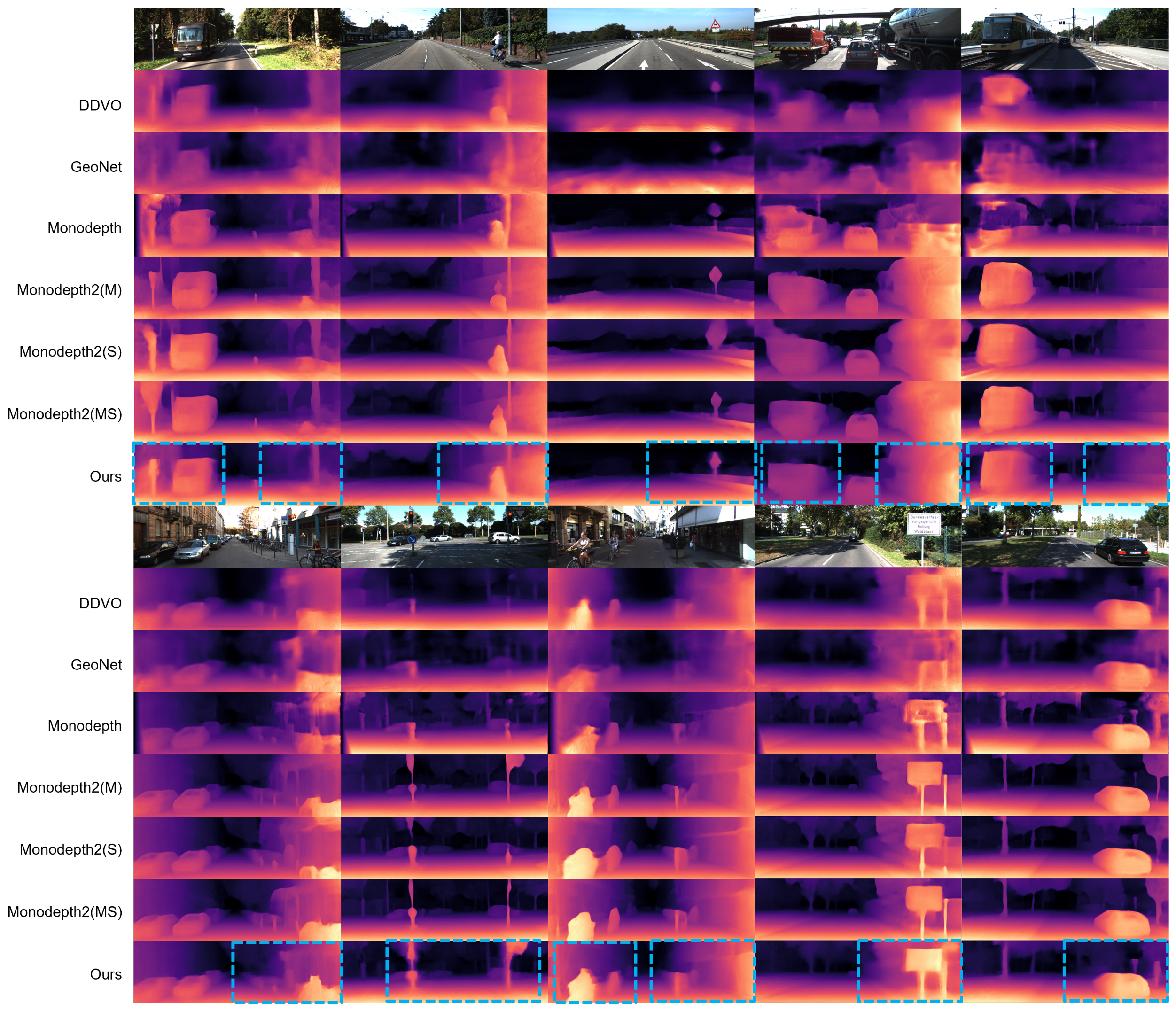
Figure 2 displays the predicted depth maps of various studies for multiple images. The comparative analysis primarily focuses on comparing our model’s results with a series of Monodepth models that share a similar structure and employ an SSIM-based image reconstruction loss. Two other relevant studies were also considered in this analysis.

In the first image of the top row, our depth map accurately represents the large bus, sign, and roadside forest on the left, as well as the grass surrounding the road and the nearby forest on the right. The second image showcases a clear depiction of a cyclist, with well-defined boundaries between the road and the trimmed shrubbery and forest in the distance. Our model’s superiority is evident in the third image, where the boundaries of roads, guardrails, low shrubbery trees, and the sky are clearly visible in the distance. The fourth image emphasizes the clear boundaries of large trucks on both sides, while the fifth image highlights the depth of a long tram on the left and the distinct border between the road, fence, and surrounding forest on the right. An important point to emphasize here is the impact of object edge clarity and object geometry correctness in the depth map on the overall depth performance. In Figure 2, the edges of objects such as cars, traffic signs, cyclists, trains, and trees in the Monodepth2(MS) images appear clearer than in our images. However, it can be observed that the shape accuracy of objects in our depth map images is higher than that of Monodepth2(MS). This difference is linked to the quantitatively enhanced performance of our model compared to Monodepth2(MS), as shown in Table 2. This means that the precise image shape of an object generated by LPIPS-based image reconstruction and left–right difference image loss functions adopted by our model has a greater impact on depth map accuracy. Evidently, further improvement is also needed to increase the accuracy of object edges in the depth map images generated by our model.

Moving to the bottom row, the first and second images provide a clearer representation of cyclists, roadside buildings, traffic lights, and signs. The third image at the bottom further demonstrates our model’s superiority, with a distinct figure of a cyclist on the left and a clearly visible outline of a large building far away on the right side of the road. In the fourth and fifth images at the bottom, our depth map accurately portrays the signs and their surroundings, as well as the cars and their surroundings. Visually, it is evident that our model generates clearer depth maps compared to other studies. Particularly, our model excels in capturing depth information for composite objects such as cyclists, large structures, distant shrubbery trees, grassy areas around roads, borders with forests, and long-distance roads. This superior performance can be attributed to the effectiveness of LPIPS-based image reconstruction loss and the inclusion of the left–right difference loss in our model.

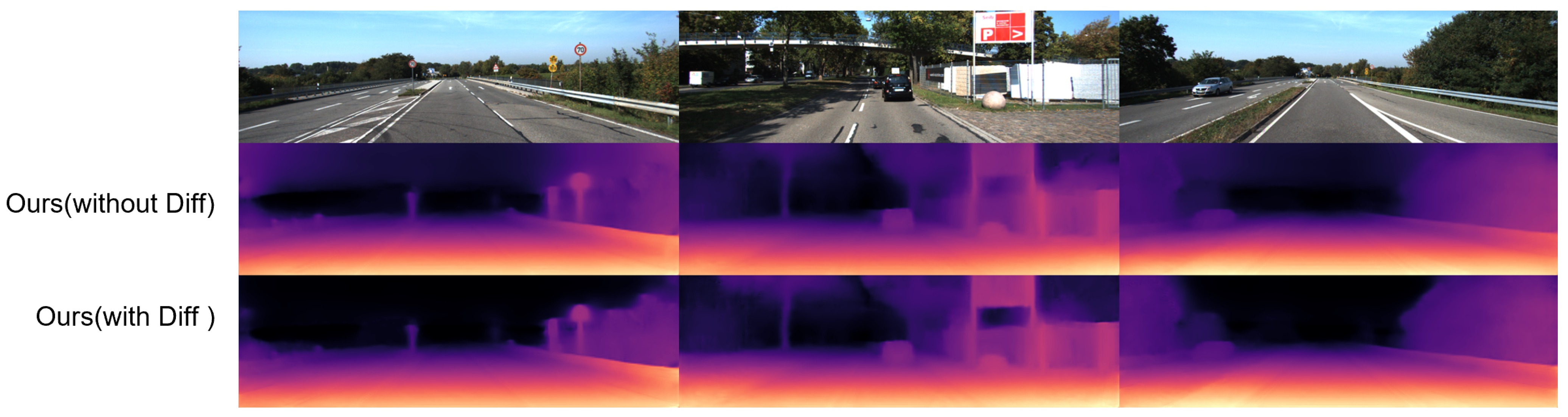
Figure 3 illustrates the impact of our model’s left–right difference image loss on the generation of depth maps for distant regions. The first depth map, positioned at the bottom, showcases the substantial improvement achieved when our model incorporates the left–right difference image loss. The boundary between the road and the guardrail is significantly clearer, even at greater distances, compared to the depth map generated by our model without utilizing this loss function. Additionally, there is an improved definition in depicting the demarcation between the forest surrounding the road and the distant sky, particularly in remote areas. The second image further highlights the difference. The model that incorporates the left–right difference image loss demonstrates enhanced clarity in distinguishing the spatial variation between the sign and the background, as well as the structure and the background, in comparison to the model without the application of this loss function. Furthermore, the third depth map reveals that the model utilizing the left–right difference image loss effectively establishes a distinct boundary between the distant forest and the sky. This demonstrates the ability of our model to capture and represent the depth information accurately, particularly in remote areas. Overall, Figure 3 emphasizes the significance of the left–right difference image loss in improving the depiction of depth maps, especially for distant regions, by enhancing clarity, spatial variation, and boundary delineation.

4.2.3. Ablation Analysis

We have conducted an ablation study with a primary focus on highlighting the efficacy of LPIPS-based image reconstruction loss and left–right difference image loss, as proposed in this paper. The ablation study also aims to offer a comparative analysis between the newly introduced LPIPS-based image reconstruction loss and the conventional SSIM-based counterpart. The outcomes of the ablation study are summarized in

Table 5. Ablation analysis (L1: L1-based image reconstruction loss, SSIM: SSIM-based image reconstruction loss, LPIPS: LPIPS-based image reconstruction loss, DIFF: left–right difference image loss, ↓: lower is better, ↑: higher is better).

Method	Abs Rel ↓	Sq Rel ↓	RMSE ↓	RMSE Log ↓	$\mathit{\delta }<1.25$↑	$\mathit{\delta }<1.{25}^2$↑	$\mathit{\delta }<1.{25}^3$↑
L1	0.178	1.213	5.601	0.250	0.735	0.922	0.970
L1 + SSIM	0.112	0.790	4.687	0.195	0.871	0.955	0.979
L1 + LPIPS	0.106	0.760	4.635	0.187	0.883	0.958	0.980
L1 + LPIPS + DIFF	0.100	0.756	4.575	0.179	0.894	0.962	0.982

.

Applying SSIM-based image reconstruction loss results in a noticeable enhancement in performance compared to using only L1 loss. Notably, the adoption of the proposed LPIPS-based image reconstruction loss yields substantial performance improvements when contrasted with the conventional SSIM-based loss. Moreover, the inclusion of the left–right difference image loss function further contributes to the overall performance enhancement. Through this comprehensive ablation analysis, we successfully demonstrate the significant effectiveness of both the proposed LPIPS-based image reconstruction loss and the left–right difference image loss.

4.3. Evaluation on CityScapes Dataset

We extensively evaluated our proposed model using a total of 1525 test images from the CityScapes dataset. To ensure methodological rigor, we applied a standardized process of cropping and resizing the lower section of each image, resulting in a uniform resolution of $640\times 192$, mirroring the approach used for the KITTI dataset. The qualitative outcomes of this evaluation, focusing on the CityScapes test images, are showcased in Figure 4. The depth maps generated by our model exhibit remarkable precision in capturing a diverse array of objects within these test images, ranging from automobiles, traffic signs, and pedestrians to trees, bicycles, and road surfaces. This impressive performance underscores the model’s robust generalization capabilities, enabling accurate depth predictions across a wide spectrum of untrained image contexts.

5. Conclusions

In conclusion, this paper presented a novel approach for self-supervised monocular depth estimation by leveraging stereo–image learning. The proposed model incorporates a perceptual assessment of reconstructed and left–right difference images, effectively guiding the training process, particularly in challenging conditions such as low-texture areas and distant regions. These kinds of regions have often posed challenges for methods utilizing conventional computer vision-based IQA models like SSIM. The adoption of LPIPS image assessment algorithm as an image reconstruction loss in our model is particularly advantageous due to its alignment with human perception during the training process. This characteristic ensures that the reconstructed images are perceptually aligned with the target images, reducing artifacts even in challenging regions. Consequently, the use of LPIPS-based loss function enhances the overall quality and visual fidelity of the reconstructed images, especially in artifact-prone regions. The integration of the left–right difference image loss primarily aims to mitigate distortions arising from variations in the left–right images of a stereo pair, caused by factors like lighting fluctuations and camera calibration errors. Moreover, the application of the left–right difference image loss effectively mitigates distortions in distant regions of the reconstructed images by guiding distant pixel values within the reconstructed difference images toward convergence with zero.

The experimental results conducted on the KITTI driving dataset provide compelling evidence of the effectiveness of our proposed approach. Our model outperforms other recent studies employing more complex approaches and those utilizing similar approaches. Despite being trained solely on stereo–image data, our model demonstrates superior performance compared to networks employing a hybrid training approach involving both stereo–image and monocular video sequence data. Furthermore, our single-task learning model trained solely for predicting depth achieves higher performance than multi-task learning models trained for both semantic segmentation and depth estimation. Through the process of comparing experimental results, we observed that the hybrid data learning and multi-task learning approaches significantly enhance the performance of self-supervised monocular depth estimation. These findings suggest that incorporating these approaches into our model has the potential to further improve its performance. As a result, our future research endeavors will focus on exploring and implementing these techniques to enhance the capabilities of our model.