Article

Combination of Fast Finite Shear Wave Transform and Optimized Deep Convolutional Neural Network: A Better Method for Noise Reduction of Wetland Test Images

1
Systems Engineering Institute, AMS, PLA, Beijing 100141, China
2
The 3rd Research Institute of China Electronics Technology Group Corporation, Beijing 100015, China
3
Xi’an Institute of Electromechanical Information Technology, Xi’an 710065, China
*
Author to whom correspondence should be addressed.
Electronics 2023, 12(17), 3557; https://doi.org/10.3390/electronics12173557
Submission received: 2 August 2023 / Revised: 9 August 2023 / Accepted: 10 August 2023 / Published: 23 August 2023
(This article belongs to the Special Issue Artificial Intelligence in Image Processing and Computer Vision)

Abstract

:
Wetland experimental images are often affected by factors such as waves, weather conditions, and lighting, resulting in severe noise in the images. In order to improve the quality and accuracy of wetland experimental images, this paper proposes a wetland experimental image denoising method based on the fast finite shearlet transform (FFST) and a deep convolutional neural network model. The FFST is used to decompose the wetland experimental images, which can capture the features of different frequencies and directions in the images. The network model has a deep network structure and powerful feature extraction capabilities. By training the model, it can learn the relevant features in the wetland experimental images, thereby achieving denoising effects. The experimental results show that, compared to traditional denoising methods, the proposed method in this paper can effectively remove noise from wetland experimental images while preserving the details and textures of the images. This is of great significance for improving the quality and accuracy of wetland experimental images.

1. Introduction

During the process of high-dimensional wetland experiments, they are often affected by harsh environmental noise, such as strong winds, insufficient lighting, rain, and snow. These factors result in a large amount of noise information being mixed in the images captured from a long distance, posing significant challenges for subsequent data analysis in the experiments. In order to address the issue of image denoising, this field has become a hot research direction in recent years. Researchers have proposed many image denoising methods and achieved good research results [1,2,3].
There are various classifications of image denoising methods, which can be broadly divided into: spatial domain-based denoising algorithms, such as Gaussian filtering [4], median filtering [5]; transform domain-based denoising algorithms, such as wavelet transform [6]; sparse representation-based denoising algorithms, such as discrete cosine transform (DCT) [7], K-singular value decomposition (K-SVD) [8]; and deep learning-based denoising algorithms, such as convolutional neural networks (CNN) [9], DnCNN [10], etc. Although existing denoising algorithms have achieved good results, they still have certain limitations. For example, median filtering often ignores important details of edges and textures during the filtering process, leading to the loss of image edges and textures. The wavelet transform, on the other hand, makes it difficult to achieve the optimal sparse representation of the geometric properties of an image on different scales. Deep learning lacks adaptive capability for handling spatially varying noise and requires training multiple network models for different noise levels. In response to these issues, in-depth research will be focused on the transform domain and deep learning aspects.
In order to achieve better sparse representation and processing of images, researchers have proposed the multiscale geometric analysis method based on the wavelet transform. By using different thresholding rules, this method achieves a hierarchical decomposition of the image from coarse-to-fine scales and has achieved excellent results in denoising. Among them, the classical ridgelet transform is a new method [11] that has better nonlinear approximation properties in two-dimensional space compared to the wavelet transform and can obtain a more efficient sparse representation. However, the performance of the ridgelet transform is not ideal when dealing with high-dimensional images, especially since the problem of wrap-around artifacts after the inverse transform still exists. To address such issues, the research on the curvelet transform by Ma et al. [12] has shown that it can effectively remove speckle and Gaussian noise while preserving the edge details of the image. However, when dealing with images with a high density of salt-and-pepper noise, this method may result in the image becoming more blurred. Senthilkumar et al. [13] proposed the use of the contourlet transform to effectively extract the geometric features and contour information of an image, and further improve the image quality. By merging singularities into the same coefficients, noise and discontinuities in the image can be reduced, resulting in clearer and smoother image results. However, there are some limitations, such as the slow convergence speed in the frequency domain and the potential problem of pseudo-oscillations. In order to address this, researchers have proposed improved methods for contourlet transform, such as nonsubsampled contourlet transform [14] and a combination of hidden Markov tree and Gaussian mixture model [15]. Zhang et al.’s research [16] introduces a novel shearlet transform method that possesses excellent time-frequency characteristics, multidirectionality, and multiscale resolution advantages. This method can more accurately capture and represent the details and structural features in an image, thereby improving the quality and clarity of the image.
In recent years, significant breakthroughs have been made in image denoising research based on deep neural networks, especially in dealing with Gaussian white noise. Tian et al. [17] combined the advantages of sparse block, feature enhancement block, attention block, and reconstruction block on the basis of CNN, which can effectively suppress noise in images. Tang et al. [18] proposed a multilayer perceptron, which achieved good results in eliminating speckle noise in images. Chen et al. [19] developed a trainable nonlinear reaction-diffusion model that can be applied to various image denoising tasks, such as Gaussian image-denoising and single-image super-resolution. However, it has been found in the research on the above model that satisfactory results cannot be obtained when dealing with noisy images of specific noise density levels, and there are certain limitations. To address this issue and improve the blind denoising capability of the model, Zhang et al. [20] proposed a combination of residual learning and batch normalization methods to accelerate the training process and enhance the Gaussian denoising capability of unknown noise. Singh et al. [21] proposed a new algorithm based on deep residual learning that can effectively overcome the problems of different levels of Gaussian noise and gradient vanishing.
Despite the significant success achieved by the multiscale geometric analysis method and deep learning methods in the field of image denoising, the current existing methods still face the following problems:
  • Most nondeep learning algorithms require prior knowledge, such as noise density levels and noise distribution. However, in real-world environments, these influencing factors are often unclear, making it difficult to achieve satisfactory denoising results using existing algorithms.
  • Multiscale geometric decomposition technique maps part of the image texture information to high-frequency sub-bands in the noise mapping process. However, when applying the threshold shrinkage method to denoise the high-frequency sub-band images, excessively high thresholds can cause the image to be excessively smoothed. This excessive smoothing phenomenon is caused by the incorrect removal of texture information in the high-frequency sub-bands, which is mistakenly identified as noise.
  • Currently, most deep learning algorithms are constructed based on known noisy prior knowledge and can only effectively denoise at specific noise density levels, typically lacking strong adaptability. Due to the network effects generated during the upsampling process, some important image details are lost.
To address the aforementioned issues, this paper proposes an image-denoising method called fast finite shearlet transform (FFST) combined with a deep convolutional neural network (CNN) model, referred to as FFSTnet [22]. Firstly, the FFST algorithm is used to decompose the original image and obtain multiple sub-band images, which are then input as training samples into the CNN network. After training the CNN denoising network, a denoising learning model is established to process the sub-band images. Finally, the inverse FFST algorithm is used to reconstruct the sub-band images and obtain the denoised image.
The main contributions of this paper are as follows:
  • A new image-denoising method based on the FFSTnet network model is proposed, which effectively overcomes the dependence of deep neural networks on large amounts of data. By decomposing the image into several sub-band images through FFST, the model still has good denoising effects with a small amount of data, and improves the model’s generalization ability.
  • Due to the excellent properties of FFST and inverse FFST transforms, no information loss occurs during image decomposition, which better preserves the texture and edge details of the image.
  • Various random training strategies are introduced during the model training process, which enables the model to handle the denoising of images with different noise density levels and actual noise, enhancing the flexibility of the model.
The remaining content of this article is as follows: The second part provides a detailed introduction to the basic theory of the fast finite shearlet transform (FFST) and convolutional neural networks (CNN). The third part describes the FFSTnet network denoising model in detail. The fourth part presents the analysis results of simulations and wetland experiments. The fifth part is the conclusion.

2. Methods

2.1. Fast Finite Shearlet Transform

When using the discrete shearlet transform (DST) method for image decomposition and reconstruction in the frequency domain [23], it may lead to the occurrence of the Gibbs phenomenon, which directly affects the effectiveness of image denoising. In order to effectively eliminate this phenomenon, this paper adopts a new method called FFST. FFST is a class of multiscale geometric analysis methods that perform well in local time-frequency processing. Compared with DST, FFST exhibits extremely rich directionality and discriminability in different scales and directions, making it better able to represent images with edges. FFST has many advantages, such as translation invariance and optimal sparse approximation, which makes it have great application prospects in image denoising, edge extraction, and other fields.
The similarities between FFST and DST in the frequency domain are that both methods involve multiscale decomposition and directional localization processes, allowing for a more comprehensive understanding and processing of image features. However, there are several differences between the two methods:
(1)
The window function W used in FFST is a function established based on the frequency domain, and its selection needs to satisfy the following conditions:
l = 2 j 2 j 1 W ˜ [ 2 j n 2 l ] = 1
(2)
In the multiscale decomposition process of FFST, a completely finite scale function is used, and its mathematical expression is:
ϕ ^ ( ω 1 , ω 2 ) = { φ ( ω 1 ) , | ω 2 | | ω 1 | φ ( ω 2 ) , | ω 1 | | ω 2 | = { 1 f o r         | ω 2 | 1 2 , | ω 1 | 1 2 cos ( π 2 υ ( 2 | ω 1 | 1 ) ) f o r         1 2 < | ω 1 | < 1 , | ω 2 | | ω 1 | cos ( π 2 υ ( 2 | ω 2 | 1 ) ) f o r         1 2 < | ω 2 | < 1 , | ω 1 | | ω 2 | 0                                                     o t h e r w i s e
In Equation (2), the form of φ ( ω ) is represented as:
φ ( ω ) = { 1   , | ω | 1 2 cos ( π 2 υ ( 2 | ω | 1 ) ) , 1 2 < | ω | 0   , | ω | > 1 1
(3)
In the process of FFST direction localization decomposition, the shear filter is used, and its mathematical expression is as follows:
w ^ j , l s [ n 1 , n 2 ] = φ p 1 ( δ ^ p [ n 1 , n 2 ] w ˜ [ 2 j n 2 l ] )
And needs to meet:
l = 2 j 2 j 1 w ^ j , l s ( ξ 1 , ξ 2 ) = 1
In Equation (4), φp represents the mapping function, where all elements Si,j need to satisfy the condition expressed by the matrix S with s i , j 2 = s i , j .
From Equation (4), it can be observed that in the implementation process of FFST, the shear filter is used with the aid of the mapping function φp to first transform from the pseudopolar coordinate domain to the Cartesian coordinate domain. However, in the Cartesian coordinate domain, a specific discrete resampling method is employed for processing in order to achieve the corresponding transformation. It is not a simple transformation.
When using inverse discrete Fourier transform, assuming w l s represents a shear filter w 0 , l s with a support domain of size L × L, for any function f l 2 ( Ζ N 2 ) , have:
j = 2 i 2 i 1 f w j s = f
According to Equation (6), it can be concluded that the shear filter constructed during the FFST transformation process is not a traditional compact support structure. In reality, we can use a matrix size much smaller than the given image size for computation. This method weakens the Gibbs phenomenon within a smaller support region and effectively improves the computational efficiency of the algorithm.

2.2. Basic Model of the Convolutional Neural Network (CNN)

2.2.1. Convolution Layer

The convolutional layer is an essential component of neural networks, and its main function is to perform convolutional operations on input images using a two-dimensional convolutional kernel. This process involves iterating through each pixel in the image and using a nonlinear activation function to solve for the feature map. Figure 1 illustrates this process. The purpose of the convolutional layer is to extract local features from the input image and adapt to different tasks and data through the parameter learning of the convolutional kernel. Through convolutional operations, neural networks can automatically learn spatial relationships and important features in images, enabling effective processing and analysis of the images.

2.2.2. Pooling Layer

After the convolutional layer, the next component in neural networks is the pooling layer, which is an important part of the network. The main purpose of the pooling layer is to downsample the input features by applying pooling kernels. This process reduces the dimensionality of the features while further extracting more valuable information. This downsampling helps to effectively reduce the number of parameters in the neural network, thereby improving the training speed of the network. In this article, the max pooling layer is used, which has the advantage of obtaining position-invariant feature parameters, as shown in Figure 2.

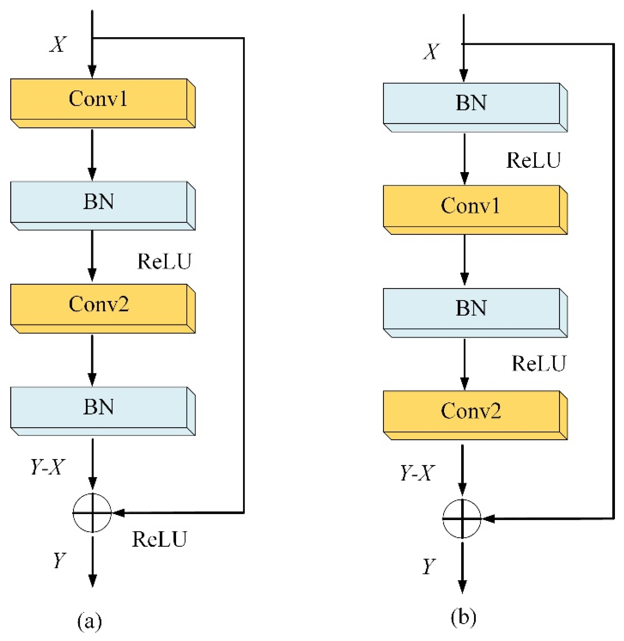
2.2.3. Residual Network

The deep residual network is a network structure composed of multiple residual blocks, which are considered the core components of the ResNet model. Here, residual refers to the difference between the observed value and the predicted value. Figure 3 shows two commonly used residual block structures. Figure 3a shows the standard residual block structure, which consists of two convolutional layers, two batch normalization layers, and two ReLU activation functions. Figure 3b shows the residual block structure with a downsampling layer, which adds a downsampling layer to the standard residual block structure. These two types of residual block structures play an important role in ResNet [24]. The residual block structure with downsampling layer provides convenience for internal backpropagation by directly connecting the input and output through a shortcut path. This structure effectively solves the problems of gradient explosion and gradient vanishing, thereby improving the training efficiency of the neural network. Given this advantage, this paper chooses to use the residual block structure with a downsampling layer as the component of the network.

2.3. Important Parameters and Optimization Methods

2.3.1. Batch Normalization

Batch normalization (BN) is an important technique that applies a unified linear transformation to the features extracted from each layer of the network. Its core idea is to normalize the features of each batch, making their mean 0 and variance 1. It is important to emphasize that this normalization is not applied to the entire layer of neurons, but to the data of each neuron independently. The advantage of BN is that it is not affected by network parameters, has good robustness, and can maintain the relative stability of the input data distribution for each layer of the network, thereby significantly improving the training speed of the network.

2.3.2. Receptive Field

The receptive field refers to the mapping of the pixels on each layer’s feature map to the area on the original image and represents the area as the size of the pixels on the feature map. This concept is crucial for understanding the visual perception and information extraction capabilities of a convolutional neural network. Through this method, we can understand which regions of the original image the pixels on the feature map are paying attention to and thus deduce the network’s sensitivity to each pixel in the image. Therefore, the size of the receptive field directly affects the network’s perception ability and its ability to capture image details.

3. Image Denoising Network Model Based on FFSTnet

3.1. The Structure of the FFSTnet Denoising Model

Figure 4 shows the network structure of the FFSTnet denoising model, which consists of a total of 15 layers in the CNN denoising network module. The size of the filter is set to 3 × 3 × a, where a = 3 represents denoising of color images, and a = 1 represents denoising of grayscale images. First, the input image is decomposed into multiple sub-band images using the FFSF transform, which not only enlarges the receptive field but also effectively enhances the denoising capability of the model. However, traditional methods of enlarging the receptive field involve increasing the size of the filter or continuously expanding the convolutional layers, resulting in higher computational costs. Among them, expanding the receptive field area through dilated convolution layers increases computational complexity and leads to the network effect. Typically, the receptive field of a CNN is set as (2N + 1) × (2N + 1), where N represents the network layer. Therefore, for a 15-layer CNN, the receptive field would be 31 × 31. After the FFST decomposition, multiple sub-band images are obtained, which increases the number of samples and allows the FFSTnet to have a receptive field of at least 66 × 66 or even larger. The FFST and inverse FFST transformations do not result in any information loss during the decomposition and reconstruction processes. This means that they effectively preserve the texture and edge details of the image. This approach not only enhances the denoising capability but also reduces the computational burden.

3.2. FFSTnet Noise Reduction Model Detailed Description

The detailed composition of each layer in the FFSTnet denoising model is as follows:
Layer 1: The input layer imports the image that needs to be denoised and uses the FFST transform to decompose it into multiple sub-band images, which serve as the data source for the second layer.
Layer 2: The convolutional layer consists of convolution (Conv) and rectified linear unit (ReLU) as activation functions, which extract feature parameters from the first layer sample images.
Layers 3–16: Composed of BN (batch normalization), ReLU, and Conv, they further extract more valuable feature parameters and complete batch normalization processing, which helps improve computational speed.
Layer 17: Composed only of Conv. After the image passes through each convolutional layer, zero-padding is performed to maintain the consistency of the sub-band image sizes.
Layer 18: Using the inverse FFST transform with the same size as the input sample, it reconstructs a series of denoised sub-images.
The number of Conv layers directly affects the performance and computational complexity of the FFSTnet denoising model. Based on the trade-off between performance and computational complexity, a denoising network with 15 layers of CNN is set according to the simulation results. Residual learning has been proven to improve computational capacity, batch normalization operations, and denoising effects. This is mainly because the output of residual learning follows a Gaussian distribution, and through multiple rounds of convolutional layer processing, it can effectively distinguish noise from structures in the image and capture more valuable feature information from specific noise levels. Therefore, residual learning has excellent denoising effects when handling single tasks with additive Gaussian white noise. To address the diversified needs of large-scale noise and single noise, different training strategy models are adopted. In Figure 4, the red arrow represents the denoising model for large-scale noise, which effectively improves the flexibility of the FFSTnet denoising model. The purple arrow represents the denoising model for additive Gaussian white noise.

3.3. FFSTnet Noise Reduction Model Important Parameter Description

The number of feature maps is a crucial parameter in the FFSTnet denoising model, as it directly affects the quality of the denoising effect. In traditional CNN models, the same number of feature maps is usually set to meet the denoising requirements of grayscale and color images. However, in the FFSTnet denoising model, only one channel is needed for grayscale images, while three channels (R, G, and B) are required for color images. Therefore, a larger number of feature maps needs to be allocated for processing color images. Based on experimental analysis, we found that setting the number of feature maps to 64 for grayscale images and 128 for color images can achieve satisfactory denoising results. This setting can better adapt to different types of image inputs and improve the performance of the denoising model.
The FFSTnet network parameters are represented by Θ. Assuming P(w; Θ) represents the output of the denoising model. Consider { ( w i , x i ) } i = 1 N as a training set, where wi represents the i-th input image and xi represents the ground truth image. For a range noise removal task, the loss function can be expressed as:
K ( Θ ) r a n g e = 1 2 N i = 1 N ( P ( w i ; Θ ) x i F 2
For a specific single task denoising model with residual learning, the loss function can be represented as:
K ( Θ ) s p e c i f i c = 1 2 N i = 1 N ( P ( w i ; Θ ) ( w i x i ) F 2
To accelerate the training process and improve the convergence speed of the FFSTnet model, we used the ADAM algorithm to optimize the network. During the network training process, the learning rate gradually decreases from 10−3 to 10−4 until the training error reaches a stable state and no longer increases. In the training phase, we set the minibatch parameter to 128 and use conventional data augmentation techniques to expand the input samples. When the training error is relatively stable in five consecutive steps, we fuse each BN parameter with the adjacent filters. Additionally, as the learning rate gradually decreases to 10−6, we also need to add an additional 50 steps to prevent the FFSTnet model from getting trapped in local minima.

4. Experimental Data Verification

4.1. Experimental Analysis of Real Image Noise Reduction

To verify the influence of different network model parameters on the image denoising effect, we selected the starfish image from the BSD68 image dataset and used the PSNR metric for objective evaluation. The main network parameter settings for the proposed FFSTnet denoising network model are shown in Table 1. When optimizing the network using the SGDM algorithm, the PSNR value is higher when the MiniBatchSize parameter is set to 128 compared to when it is set to 64, indicating a better denoising effect. When optimizing the network using the ADAM algorithm and setting the MiniBatchSize parameter to 128, the PSNR metric is significantly higher than the results of other parameters, effectively verifying the effectiveness of the FFSTnet network parameter settings.
In terms of model training, the ImageNet dataset is used as the training sample. In the experiment, FFSTnet uses 300 images as the training sample, and cuts the input sample picture into 128 × 2000 image blocks of 50 × 50, so that the model can obtain good generalization performance.

4.2. Simulation Experiment Analysis of Grayscale Image Denoising

4.2.1. Compared with Traditional Methods

The effectiveness of the proposed FFSTnet denoising method was validated in two dimensions: traditional and classical deep learning denoising algorithms, as shown in Table 2. In terms of validation datasets, BSD68 and Set12 were used, and the noise density parameter in each denoising algorithm was uniformly set to (σ = 15 for low density, 25 for medium density, 50 for high density). The objective evaluation selects the peak signal-to-noise ratio (PSNR) metric as the criterion for judging the denoising effect.
From Figure 5, Figure 6 and Figure 7, it can be seen that when using the Meanfilter and Medianfilter denoising algorithms to process the image, the texture details of the image will become blurred, resulting in the occurrence of artifacts. This phenomenon will increase the blurriness of the image as the noise density parameter increases. In the river image with σ = 50, the recognition of the river and land in the enlarged area is very low.
Secondly, from the perspective of visual effects, the denoising algorithms K-SVD and BM3D are obviously superior to the Meanfilter and Medianfilter denoising algorithms, but the problems of blurry texture details and artifacts still exist. Compared to the previous algorithms, the DnCNN denoising algorithm can effectively remove noise interference in the image, thereby obtaining a clearer image.
Finally, under three different noise density conditions, the FFSTnet denoising algorithm proposed in this paper is compared with five other algorithms. This method can effectively preserve the edge texture details of the image and achieve good denoising results. The train head and smoke in Figure 5 and the river and land in Figure 7 can be clearly distinguished. This is because FFST and inverse FFST have many excellent characteristics, which enable FFSTnet to have a strong ability to preserve image details and achieve ideal denoising results.

4.2.2. Signal-to-Noise Ratio Analysis of the Denoising Effect

To further validate the effectiveness of this method, we selected some images from the BSD68 and Set12 image datasets and conducted objective evaluations using the PSNR metric, as shown in Table 3. Through the analysis of Table 3, the following conclusions can be summarized:
  • Compared to the Meanfilter and Medianfilter denoising algorithms, the proposed FFSTnet denoising model in this paper has improved PSNR values by 5.14 dB and 5.41 dB, respectively, at σ = 15. This represents a significant improvement in image denoising, indicating that traditional filtering-based denoising algorithms cannot effectively preserve the texture information of the image in nonsmooth areas, resulting in poor denoising performance. Compared to deep learning algorithms, the FFSTnet model demonstrates better capability in extracting image features, leading to more ideal denoising results.
  • Compared to the K-SVD and BM3D algorithms, the PSNR values of the proposed method generally improved by 0.19–4.24 dB, demonstrating good denoising performance. Firstly, the K-SVD denoising algorithm has a strong adaptive learning capability, which can effectively compensate for the limitations of traditional dictionary matrix bases in adapting to image textures and achieve good denoising results. However, a drawback is that it requires a large amount of computational power for dictionary updates. Secondly, the core idea of the BM3D denoising algorithm is to use search image similar blocks to filter in the transform domain, obtain a large number of overlapping local block estimates, and perform weighted averaging to achieve good denoising results. However, the proposed FFSTnet denoising model demonstrates a good ability to obtain optimal representations containing texture, contours, edges, etc., at different scales, directions, and resolutions when dealing with images with regular repetitive structures, resulting in decent denoising performance. Conversely, for images with irregular textures, this specific prior advantage may be lost, leading to suboptimal denoising results.
  • Compared to the DnCNN denoising algorithm, the denoising performance of the FFSTnet model improved by 0.17 dB, 0.22 dB, and 0.27 dB, respectively, at σ = 15, 25, and 50, indicating that the FFSTnet model has better denoising capabilities under the same noise conditions, surpassing DnCNN. This is because when FFSTnet decomposes the image, the region size exceeds that of DnCNN. The larger the receptive field area, the more valuable spatial features and texture information can be extracted, which to some extent improves the denoising performance of the FFSTnet model.
  • Compared with the DSTnet algorithm, when σ = 15, 25, and 50, the noise reduction effect is improved by 0.09 db, 0.09 db, and 0.05 db, respectively, which proves that the FFSTnet model has a better noise reduction effect than the DSTnet model because FFST is superior to DST in the characteristics of directional localization, different scales, and different directions.
  • From the perspective of the average PSNR values, it is evident that the FFSTnet denoising model has higher PSNR values than other denoising algorithms under different noise conditions. A higher PSNR value indicates better denoising performance. The PSNR values are 33.34 dB, 30.99 dB, and 27.92 dB, respectively, further demonstrating the effectiveness of the proposed method.
However, in addition to PSNR evaluation indicators, there are many other image quality evaluation indicators, such as perceptual similarity (PSIM) [27], structural similarity (SSIM) [28], and so on. From the observation of Table 4, it can be clearly seen that when σ = 15, the FFSTnet noise reduction model is higher than DSTnet and DnCNN in the PSIM and SSMI evaluation indexes. The larger the value of SSMI, the better the quality of the noise reduction image; conversely, the smaller the value of SSMI, the worse the quality of the noise reduction image. From the average value, the noise reduction effect of FFSTnet is also better than the other two algorithms, which further proves the effectiveness of the proposed method in this paper.

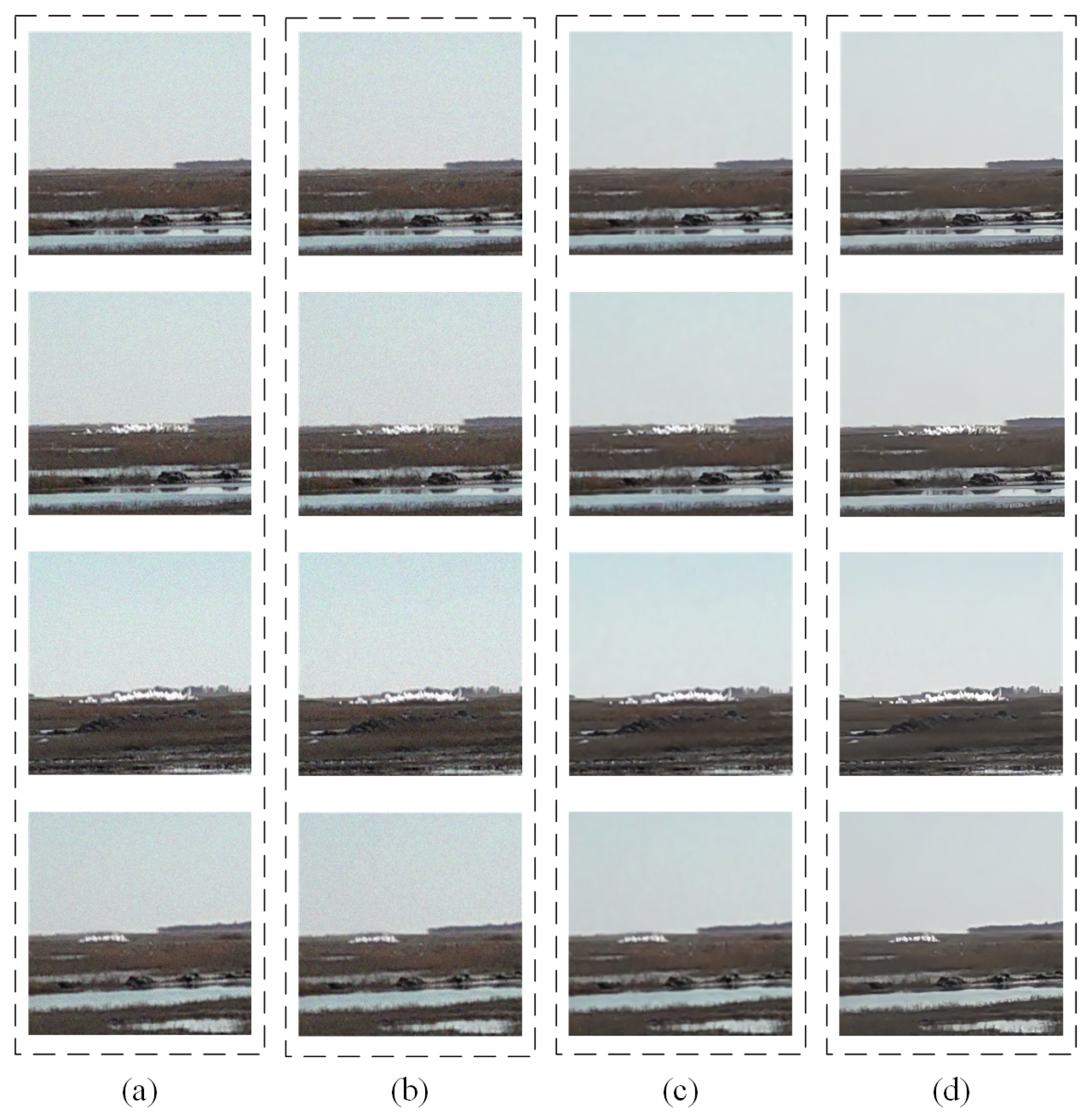
4.3. Experimental Analysis of Real Image Noise Reduction

To validate the effectiveness of the FFSTnet denoising model in practical applications, actual image samples containing noise will be used to compare the actual denoising performance of the FFSTnet model. Considering the various sources of noise in actual noisy images, such as image acquisition, compression, and the external environment, it is important to note that the noise exhibits characteristics such as spatial variation and non-Gaussian distribution. Currently, there is no accurate objective evaluation metric to assess denoising performance. Therefore, a subjective visual evaluation method will be used to compare the denoising results.

4.3.1. Comparative Analysis of Noise Reduction in Gray Level Image

In this paper, we selected the K-SVD, BM3D, DnCNN, and MWCNN [29] denoising algorithms for comparative analysis. The image dataset used was grayscale images with different noise densities from the RENIOR dataset in order to further validate the effectiveness of the FFSTnet denoising model. Through the analysis of Figure 8, the following conclusions can be summarized:
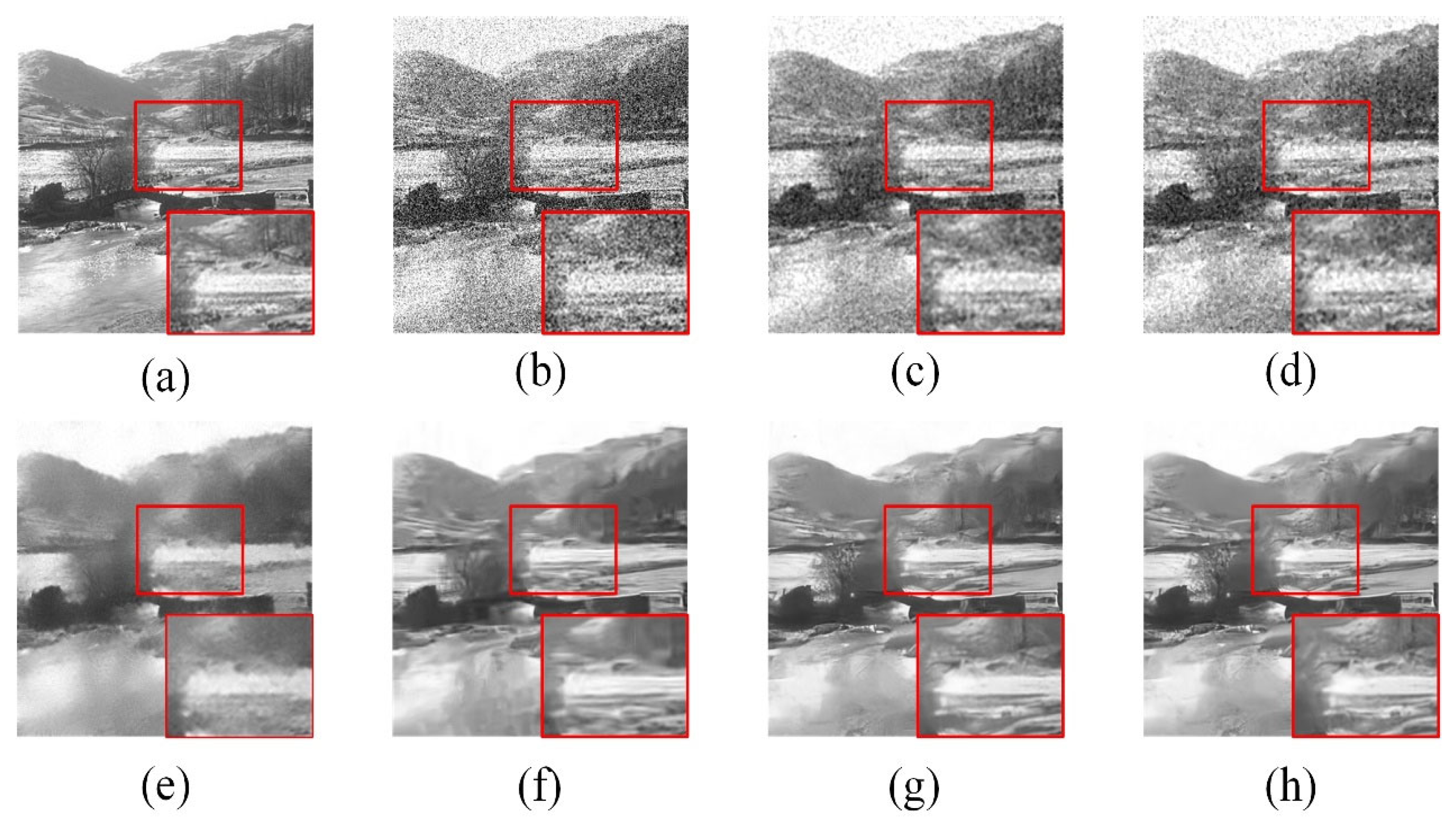
  • Each denoising algorithm achieved the expected results when denoising the third image. Secondly, K-SVD and BM3D denoising algorithms performed poorly when denoising the first, second, and fourth images in Figure 7. In comparison, the denoising effect of the FFSTnet denoising model on these images was significantly better than that of DnCNN and MWCNN. However, it should be noted that both FFSTnet and MWCNN exhibited over-smoothing in certain cases, which means that these two methods may partially lose the fine details of the image.
  • The overall denoising performance of K-SVD and BM3D algorithms on real noisy images was poor. The main reason for this result is that the K-SVD algorithm has limited denoising effectiveness on the texture and edge parts of high-frequency and low-frequency images when optimizing the dictionary. Although the K-SVD algorithm performs well in some specific scenarios, it has certain limitations when dealing with images containing nonrepetitive structural noise. On the other hand, the BM3D algorithm denoises by utilizing the similarity between blocks. However, when processing images with nonrepetitive structural noise, the characteristics of this noise result in the low similarity between blocks, which affects the denoising effectiveness of the BM3D algorithm.
  • Compared to DnCNN, MWCNN achieved better denoising performance. This result is mainly attributed to the excellent time-frequency localization characteristics and detail preservation ability of the discrete wavelet transform (DWT) used in MWCNN. Additionally, DWT can effectively balance the size of the receptive field and improve computational efficiency, thereby further enhancing the denoising effectiveness.
In conclusion, the proposed FFSTnet denoising model in this paper demonstrates stable denoising capabilities in practical grayscale noisy image applications. Compared to other denoising algorithms, the reason for this stability lies in the fact that the denoising model uses random-range noise during training. This strategy effectively eliminates Gibbs artifacts and noise in the image while preserving more texture and detail elements.

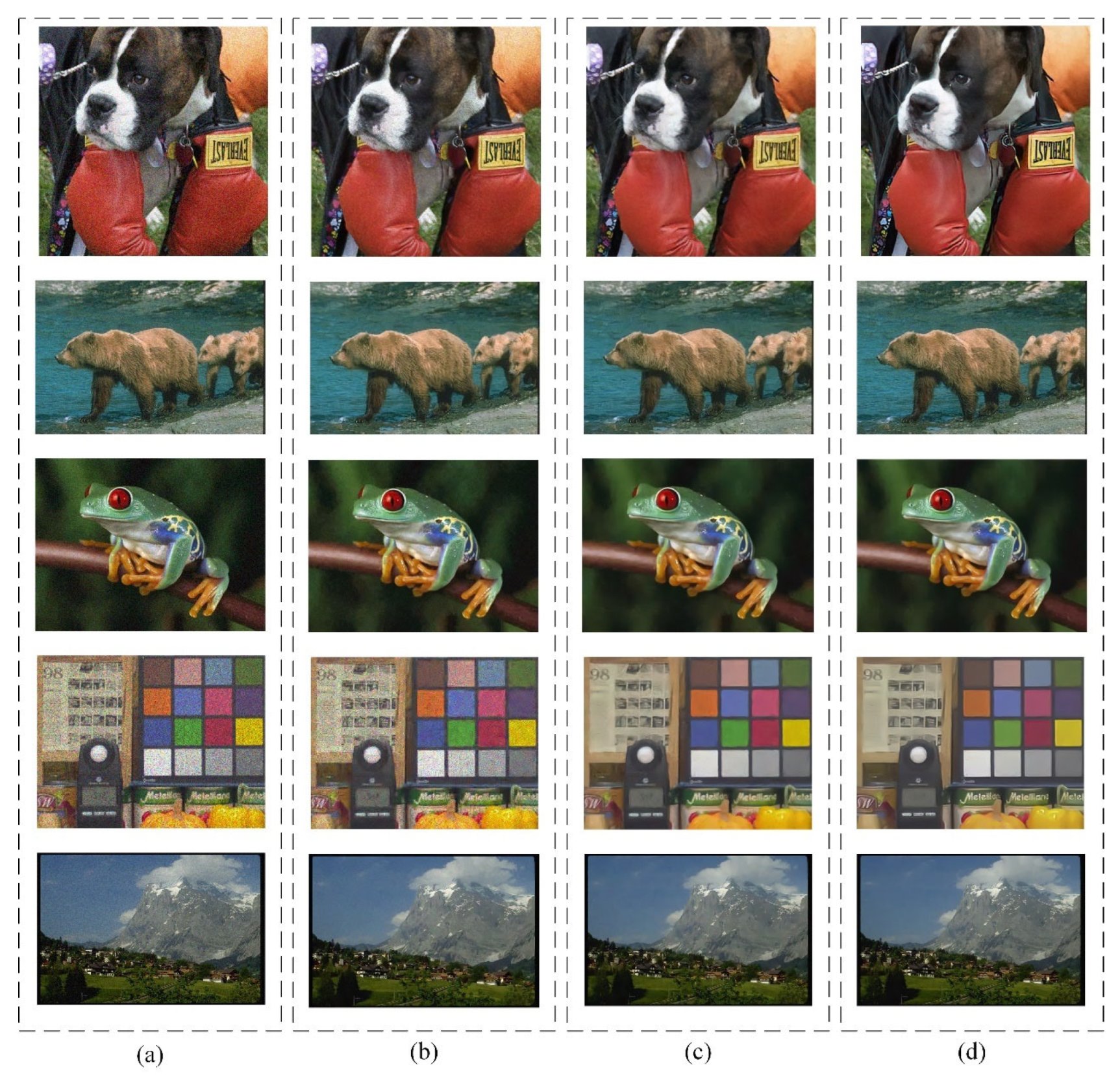
4.3.2. Contrastive Analysis of Noise Reduction in Color Images

In this study, we selected CBM3D and DnCNN as the two denoising algorithms for comparative analysis. To validate the effectiveness of the FFSTnet denoising model, we used color images with different noise densities from the RENIOR dataset as samples, as well as actual wetland experimental image data. By conducting experiments on these samples, we can verify the performance of the FFSTnet denoising model.
From the results in Figure 9, it can be observed that, compared to the CBM3D algorithm, both DnCNN and FFSTnet denoising algorithms exhibit better denoising performance. This further validates the ineffectiveness of denoising algorithms that rely on nonlocal similarity to remove noise in actual images. Compared to DnCNN, the images denoised by DnCNN appear overly smooth in texture details and edge parts. Therefore, there is still room for improvement and optimization in selecting methods to preserve image detail elements and eliminate noise. The FFSTnet denoising model proposed in this study demonstrates excellent denoising performance when dealing with actual noisy images. From a subjective visual perspective, the texture of the denoised images is very clear, successfully removing the noise components from the images.
From the observed actual wetland experimental image data in Figure 10, it is evident that the CBM3D algorithm performs poorly in terms of denoising results and fails to effectively remove noise from all images. This further demonstrates the limited adaptability of algorithms relying on nonlocal similarity in noisy image applications. Although both DnCNN and FFSTnet algorithms can effectively remove noise from the actual images by observing the clarity of the wetland and distant smoke in all images, it is apparent that FFSTnet outperforms DnCNN in terms of denoising effectiveness. This indicates that the FFSTnet denoising model can more accurately capture and restore texture details and edge features in actual noisy images, making it better suited for applications in different noise environments.
In conclusion, through experiments on publicly available image datasets and wetland experimental data, the FFSTnet denoising model has demonstrated excellent denoising capabilities, further validating the effectiveness and robustness of this method.

4.4. Analysis of Computational Speed

Computational speed is also an important criterion in evaluating denoising algorithms. Table 5 presents the computation times of BM3D, DnCNN, MWCNN, and FFSTnet. The speed of computation is closely related to the size of the image, with smaller images resulting in faster computation speeds, while larger images require more computation time. The denoising computation times for grayscale and color images of three different sizes are compared and analyzed: 1024 × 1024, 512 × 512, and 256 × 256. The experiments were conducted on a computer with a 12-core Intel(R) Core(TM) i7-8750H @ 2.20 GHz processor, 32 GB RAM, and Nvidia GeForce GTX 1050 Ti 4 GB, all running on the Matlab(R2020b) environment. Based on the observation and analysis of Table 5, the following conclusions can be drawn:
  • When removing noise from color images, all denoising algorithms require more time compared to processing grayscale images. This is because color images contain richer information, and the transformation of luminance and chrominance components requires more computational resources to support.
  • DnCNN, MWCNN, and FFSTnet can effectively harness the powerful computing capabilities of GPUs. However, for the BM3D model, there is a lack of GPU acceleration support when processing color images, resulting in suboptimal computational speed.
  • The FFSTnet denoising model performs exceptionally well in handling noise in both grayscale and color images, requiring the shortest processing time. Additionally, the model not only exhibits flexibility to adapt to various practical application scenarios, but also demonstrates outstanding denoising effectiveness. Therefore, FFSTnet has extensive application value and strong competitiveness in solving real-world problems.

5. Conclusions

To address the common lack of flexibility in deep learning denoising models and the difficulty of modeling through small samples. This study proposes an image-denoising method that combines the FFST with a deep convolutional neural network (CNN) model. By decomposing the image using FFST, the number of samples for each image is increased, and then a superior network model is obtained through deep learning. This overcomes the problem of overfitting in small-sample model training and improves the generalization ability of the model. To achieve denoising with FFSTnet for different noise levels, multiple random learning strategies are employed to enhance the adaptability of the model. The simulation results show that the proposed model achieves a good balance between denoising effectiveness and preserving image edge details. The results on real noisy images validate that the proposed model achieves good subjective and objective evaluations, effectively addressing spatially variant noise problems. Comparisons of computational time indicate that the FFSTnet denoising network model has the advantages of fast speed and low computational complexity compared to other algorithms. The research results will provide a new idea and method for solving the noise problem in the complex background. In the next step, we will carry out in-depth research on practical engineering applications.

Author Contributions

Data curation, X.C. and Y.Z.; Resources, Y.Z. and Z.W.; Supervision, X.C.; Validation, X.C. and H.B.; Writing—original draft, X.C.; Writing—review & editing, X.C. All authors have read and agreed to the published version of the manuscript.

Funding

This research received no external funding.

Data Availability Statement

Data will be provided upon request to the authors.

Conflicts of Interest

The authors declare no conflict of interest.

References

  1. Sun, H.; Peng, L.; Zhang, H.; He, Y.; Cao, S.; Lu, L. Dynamic PET image denoising using deep image prior combined with regularization by denoising. IEEE Access 2021, 9, 52378–52392. [Google Scholar] [CrossRef]
  2. Tran, T.O.; Vo, T.H.; Le, N.Q.K. Omics-based deep learning approaches for lung cancer decision-making and therapeutics development. Brief. Funct. Genom. 2023, 7, elad031. [Google Scholar] [CrossRef] [PubMed]
  3. Yuan, Q.; Chen, K.; Yu, Y.; Le, N.Q.K.; Chua, M.C.H. Prediction of anticancer peptides based on an ensemble model of deep learning and machine learning using ordinal positional encoding. Brief. Bioinform. 2023, 24, bbac630. [Google Scholar] [CrossRef] [PubMed]
  4. Shi, K.; Guo, Z. Non-Gaussian Noise Removal via Gaussian Denoisers with the Gray Level Indicator. J. Math. Imaging Vis. 2023, 1–17. [Google Scholar] [CrossRef]
  5. Li, P.; Liu, X.; Xiao, H. Quantum image median filtering in the spatial domain. Quantum Inf. Process. 2018, 17, 49. [Google Scholar] [CrossRef]
  6. Maria, H.H.; Jossy, A.M.; Malarvizhi, G.; Jenitta, A. Analysis of lifting scheme based double density dual-tree complex wavelet transform for de-noising medical images. Optik 2021, 241, 166883. [Google Scholar] [CrossRef]
  7. Lin, Z.; Jia, S.; Zhou, X.; Zhang, H.; Wang, L.; Li, G.; Wang, Z. Digital holographic microscopy phase noise reduction based on an over-complete chunked discrete cosine transform sparse dictionary. Opt. Lasers Eng. 2023, 166, 107571. [Google Scholar] [CrossRef]
  8. Ma, X.; Hu, S.; Liu, S. SAR image de-noising based on shift invariant K-SVD and guided filter. Remote Sens. 2017, 9, 1311. [Google Scholar] [CrossRef]
  9. Cho, S.I.; Kang, S.J. Gradient prior-aided CNN denoiser with separable convolution-based optimization of feature dimension. IEEE Trans. Multimed. 2018, 21, 484–493. [Google Scholar] [CrossRef]
  10. Hsu, L.Y.; Hu, H.T. QDCT-based blind color image watermarking with aid of GWO and DnCNN for performance improvement. IEEE Access 2021, 9, 155138–155152. [Google Scholar] [CrossRef]
  11. Arivazhagan, S.; Ganesan, L.; Kumar, T.G.S. Texture classification using ridgelet transform. Pattern Recognit. Lett. 2006, 27, 1875–1883. [Google Scholar] [CrossRef]
  12. Ma, J.; Plonka, G. The curvelet transform. IEEE Signal Process. Mag. 2010, 27, 118–133. [Google Scholar] [CrossRef]
  13. Senthilkumar, M.; Periasamy, P.S. RETRACTED: Contourlet transform and adaptive neuro-fuzzy strategy–based color image watermarking. Meas. Control 2020, 53, 287–295. [Google Scholar] [CrossRef]
  14. Wang, X.; Zhang, S.; Wen, T.; Yang, H.; Niu, P. Coefficient difference based watermark detector in nonsubsampled contourlet transform domain. Inf. Sci. 2019, 503, 274–290. [Google Scholar] [CrossRef]
  15. Po, D.D.Y.; Do, M.N. Directional multiscale modeling of images using the contourlet transform. IEEE Trans. Image Process. 2006, 15, 1610–1620. [Google Scholar] [CrossRef]
  16. Zhang, H.; Cheng, J.; Tian, M.; Liu, J.; Shao, G.; Shao, S. A Reverberation Noise Suppression Method of Sonar Image Based on Shearlet Transform. IEEE Sens. J. 2022, 23, 2672–2683. [Google Scholar] [CrossRef]
  17. Tian, C.; Xu, Y.; Li, Z.; Zuo, W.; Fei, L.; Liu, H. Attention-guided CNN for image denoising. Neural Netw. 2020, 124, 117–129. [Google Scholar] [CrossRef]
  18. Tang, X.; Zhang, L.; Ding, X. SAR image despeckling with a multilayer perceptron neural network. Int. J. Digit. Earth 2019, 12, 354–374. [Google Scholar] [CrossRef]
  19. Chen, Y.; Pock, T. Trainable nonlinear reaction diffusion: A flexible framework for fast and effective image restoration. IEEE Trans. Pattern Anal. Mach. Intell. 2016, 39, 1256–1272. [Google Scholar] [CrossRef]
  20. Zhang, K.; Zuo, W.; Chen, Y.; Meng, D.; Zhang, L. Beyond a gaussian denoiser: Residual learning of deep cnn for image denoising. IEEE Trans. Image Process. 2017, 26, 3142–3155. [Google Scholar] [CrossRef]
  21. Singh, G.; Mittal, A.; Aggarwal, N. ResDNN: Deep residual learning for natural image denoising. IET Image Process. 2020, 14, 2425–2434. [Google Scholar] [CrossRef]
  22. Yu, X.; Cui, Y.; Wang, X.; Zhang, J. Image fusion algorithm in integrated space-ground-sea wireless networks of B5G. EURASIP J. Adv. Signal Process. 2021, 2021, 55. [Google Scholar] [CrossRef]
  23. Lyu, Z.; Zhang, C.; Han, M. DSTnet: A new discrete shearlet transform-based CNN model for image denoising. Multimed. Syst. 2021, 27, 1165–1177. [Google Scholar] [CrossRef]
  24. Agis, D.; Pozo, F. Vibration-Based Structural Health Monitoring Using Piezoelectric Transducers and Parametric t-SNE. Sensors 2020, 20, 1716. [Google Scholar] [CrossRef]
  25. Bnou, K.; Raghay, S.; Hakim, A. A wavelet denoising approach based on unsupervised learning model. EURASIP J. Adv. Signal Process. 2020, 2020, 36. [Google Scholar] [CrossRef]
  26. Dabov, K.; Foi, A.; Katkovnik, V.; Egiazarian, K. Image denoising by sparse 3-D transform-domain collaborative filtering. IEEE Trans. Image Process. 2007, 16, 2080–2095. [Google Scholar] [CrossRef]
  27. Gu, K.; Li, L.; Lu, H.; Min, X.; Lin, W. A fast reliable image quality predictor by fusing micro- and macro-structures. IEEE Trans. Ind. Electron. 2017, 64, 3903–3912. [Google Scholar] [CrossRef]
  28. Wang, Z.; Bovik, A.C.; Sheikh, H.R.; Simoncelli, E.P. Image quality assessment: From error visibility to structural similarity. IEEE Trans. Image Process. 2004, 13, 600–612. [Google Scholar]
  29. Liu, P.; Zhang, H.; Zhang, K.; Lin, L.; Zuo, W. Multi-level wavelet-CNN for image restoration. In Proceedings of the IEEE Conference on Computer Vision and Pattern Recognition Workshops, Salt Lake City, UT, USA, 18–22 June 2018; pp. 773–782. [Google Scholar]
Figure 1. Schematic diagram of the convolution process.
Electronics 12 03557 g001
Figure 2. Schematic diagram of the convolution process.
Electronics 12 03557 g002
Figure 3. Schematic diagram of residual structure block: (a) identity residual block; (b) sampling residual block.
Electronics 12 03557 g003
Figure 4. Network structure of FFSTnet noise reduction model.
Electronics 12 03557 g004
Figure 5. Denoising results of a train image with noise density σ = 15: (a) original image; (b) noisy image = 23.15 db; (c) Meanfilter = 23.79 db; (d) Medianfilter = 23.76 db; (e) K−SVD = 28.72 db; (f) BM3D = 29.66 db; (g) DnCNN = 29.99 db; and (h) FFSTnet = 30.06 db.
Electronics 12 03557 g005
Figure 6. Denoising results of a ship image with noise density σ = 25: (a) original image; (b) noisy image = 20.32 db; (c) Meanfilter = 26.55 db; (d) Medianfilter = 25.73 db; (e) K−SVD = 27.91 db; (f) BM3D = 29.82 db; (g) DnCNN = 30.20 db; and (h) FFSTnet = 30.24 db.
Electronics 12 03557 g006
Figure 7. Denoising results of a river image with noise density σ = 50: (a) original image; (b) noisy image = 14.16 db; (c) Meanfilter = 21.52 db; (d) Medianfilter = 20.40 db; (e) K−SVD = 22.74 db; (f) BM3D = 23.90 db; (g) DnCNN = 24.29 db; and (h) FFSTnet = 24.35 db.
Electronics 12 03557 g007
Figure 8. Comparative analysis of noise reduction effect of gray image: (a) original noise image; (b) K-SVD; (c) BM3D; (d) DnCNN; (e) MWCNN; and (f) FFSTnet.
Electronics 12 03557 g008
Figure 9. Comparative analysis of noise reduction effect of color images: (a) original image with noise; (b) BM3D; (c) DnCNN; and (d) FFSTnet.
Electronics 12 03557 g009
Figure 10. Comparative analysis of noise reduction effect of color images in the wetland test: (a) original noisy image; (b) CBM3D; (c) DnCNN; and (d) FFSTnet.
Electronics 12 03557 g010
Table 1. Comparison of different network parameters.
FFSTnetFFSTnetFFSTnetFFSTnet
Solver name (algorithm)sgdmsgdmadamadam
InitialLearnRate0.00050.00050.00050.0005
MaxEpochs30303030
MiniBatchSize6412864128
ValidationFrequency50505050
ShuffleEvery epochEvery epochEvery epochEvery epoch
ExecutionEnvironmentGPUGPUGPUGPU
PSNR31.35 db32.27 db33.62 db35.12 db
Table 2. List of traditional noise reduction methods.
No.Noise Reduction MethodType
1Mean filteringBelongs to linear filtering and denoising methods
2Median filteringBelongs to nonlinear filtering and denoising methods
3K-SVD [25]Belongs to adaptive overcomplete dictionary denoising methods
4BM3D [26]Belongs to nonlocal similarity denoising methods
5DnCNN [20]Belongs to discriminative learning denoising methods
Table 3. The PSNR (db) of different methods on datasets BSD68 and Set12.
ImagesStarfishHousetest002test003test018test042Ave.
Noise level σ = 15
Meanfilter29.9827.5927.8925.8530.6526.1028.01
Medianfilter29.7127.7427.9125.9129.9926.2527.92
K-SVD33.2229.5830.8430.8233.2030.2231.31
BM3D34.9334.8734.9735.0335.0335.0034.97
DnCNN34.9532.0332.6832.5235.2532.0333.24
DSTnet35.0332.0632.7132.5735.2832.0933.29
FFSTnet35.1232.1432.7332.6035.3332.1333.34
Noise level σ = 25
Meanfilter27.5126.0226.4624.7628.0424.9726.29
Medianfilter26.4825.3125.8424.3026.8224.4925.54
K-SVD30.6526.8528.2528.0630.6627.9228.73
BM3D28.5728.5628.6028.5028.4728.5728.55
DnCNN33.0829.3530.2230.0733.0629.6530.91
DSTnet33.2129.3730.2430.0933.1029.6630.94
FFSTnet33.3029.4030.2730.1233.1429.6930.99
Noise level σ = 50
Meanfilter22.7622.2722.8521.7323.0721.8522.42
Medianfilter21.3321.0021.4920.5521.5820.6321.10
K-SVD26.0422.9025.5424.2827.7724.3925.15
BM3D26.6226.6426.6326.6526.6526.6526.64
DnCNN30.0125.7527.2826.9330.3626.6827.84
DSTnet30.2325.7727.2926.8930.4126.6927.88
FFSTnet30.2825.7927.3126.9430.5026.7127.92
Table 4. When σ = 15, different image quality evaluation indexes are compared and analyzed.
IndicatorsPSIMSSIM
MethodsFFSTnetDSTnetDnCNNFFSTnetDSTnetDnCNN
Starfish0.99920.99860.99810.94490.94450.9422
House0.99830.99790.99750.88760.88730.8855
test0020.99850.99800.99760.91830.91760.9148
test0030.99880.99830.99770.92140.92020.9171
test0180.99870.99820.99730.95250.95170.9493
test0420.99770.99740.99720.91120.90960.9088
Ave.0.99850.99810.99760.92270.92180.9196
Table 5. Calculation time of different noise reduction algorithms (seconds).
SizeBM3DDnCNNMWCNNFFSTnet
GrayColorGrayColorGrayColorGrayColor
DeviceCPUGPUGPUGPU
256 × 2560.671.360.0190.0220.0670.0770.0140.013
512 × 5122.854.230.0390.0510.1090.1860.0220.029
1024 × 102410.6122.740.1350.1630.3720.4310.0430.051
Disclaimer/Publisher’s Note: The statements, opinions and data contained in all publications are solely those of the individual author(s) and contributor(s) and not of MDPI and/or the editor(s). MDPI and/or the editor(s) disclaim responsibility for any injury to people or property resulting from any ideas, methods, instructions or products referred to in the content.

