A Sales Forecasting Model for New-Released and Short-Term Product: A Case Study of Mobile Phones

Abstract

In today’s competitive market, sales forecasting of newly released and short-term products is an important challenge because there is not enough sales data. To address these challenges, we propose a sales forecasting model for new-released and short-term products and study the case of mobile phones. The main approach is to develop an integrated sales forecasting model by training the sales patterns and product characteristics of the same product category. In particular, we analyze the performance of the latest 12 machine learning models and propose the best performance model. Machine learning models have been used to compare performance through the development of Ridge, Lasso, Support Vector Machine (SVM), Random Forest, Gradient Boosting Machine (GBM), AdaBoost, LightGBM, XGBoost, CatBoost, Deep Neural Network (DNN), Recurrent Neural Network (RNN), and Long Short-Term Memory (LSTM). We apply a dataset consisting of monthly sales data of 38 mobile phones obtained in the Korean market. As a result, the Random Forest model was selected as an excellent model that outperforms other models in terms of prediction accuracy. Our model achieves remarkable results with a mean absolute percentage error (MAPE) of 42.6258, a root mean square error (RMSE) of 8443.3328, and a correlation coefficient of 0.8629.

1. Introduction

The current economic situation is characterized by intense competition, rapid product development, and increased product differentiation, resulting in shorter product lifecycles and greater volatility in sales patterns. These changes have significant implications for the retail industry, which faces stronger requirements for sales forecasting. In the industry, accurate sales forecasting is becoming increasingly important because if excessive sales forecasting is made, malicious inventory will accumulate, and if under-sales forecasting is made, the opportunity to increase profits will be lost. In particular, as the life cycle of the product is getting shorter, sales forecasting immediately after release is becoming very important. However, forecasting sales for newly released and short-term products is challenging because of the limited availability of historical sales data, a major source of sales forecasting. In particular, sectors such as electronics and fashion encounter challenges in accurately forecasting sales due to high product diversity and limited sales history [1]. Even with business expertise, predictions can still be influenced by cognitive and motivational biases [2,3]. Additionally, while it is known that there is some kind of nonlinear mapping relationship between sales series, it is difficult to explain it with a clear mathematical model. For the above reasons, machine learning models are suitable for learning and predicting quantitative data-based linear and nonlinear sales patterns.

While individual forecasting models of short-term products may face learning failures and generalization errors due to limited amounts and diversity of data, integrated models across short-term product groups can achieve stronger results. Given the shorter product lifecycles of products like mobile phones [4], an integrated model for the product group is more appropriate. In particular, when the amount of data is limited, such as short-term products, machine learning, which is less affected by data sets, should be considered first rather than deep learning, which requires relatively much data [5]. Product sales forecasting is influenced by various factors, and past sales are one of the factors that are usually considered [6,7,8]. However, in order to build an integrated model for short-term products, identifying the characteristics between products can also be an important factor. Therefore, in this study, we develop an integrated sales forecasting model for mobile phones, taking into account various data on product sales and context, including when to introduce, specifications provided by manufacturers, and information on product sales.

Sales forecasting has been extensively explored by researchers, encompassing various topics and methodologies. Notably, a range of methods for sales and demand forecasting have been studied, with a recent emphasis on machine learning and deep learning models. In one study, multiple linear regression and Support Vector Machine (SVM) were applied to forecast sales in the German automobile market. The results demonstrated that the nonlinear SVM model outperformed the linear regression model [9]. Another study investigated traffic accidents and employed Linear Regression, Random Forest, Naive Bayesian, and AdaBoost. Among these models, Random Forest yielded the best performance [10]. An empirical study focused on predicting tourism demand for Hong Kong visitors using the Lasso model, which was found to be valid for this purpose [11]. Another study analyzed supply chain demand forecasts using nonlinear machine learning techniques, specifically SVM and Recurrent Neural Network and demonstrated their superiority over traditional statistical methods when applied to real Canadian foundry data [12]. Additionally, a study predicted retail clothing sales using SVM and artificial neural networks, revealing that the models based on artificial neural networks outperformed SVM [13]. Moreover, Support Vector Regression was employed to forecast demand for Taiwanese mobile phones, further highlighting its effectiveness [14].

Tree-based ensemble models have also been extensively explored in demand forecasting. For example, Reference [15] presented gradient boosting models trained on different aggregations of water consumption data, emphasizing the impact of spatial aggregation on forecasting accuracy. The study also indicated that the incorporation of additional explanatory variables can minimize forecasting errors. Similarly, GBM and LightGBM were assessed for their utility in forecasting future sales and promotions, demonstrating decent accuracy [16,17,18]. XGBoost, a widely used model in demand forecasting due to its strong performance in sales forecasting for retail, was found to be a favorable choice [19]. The performance of XGBoost surpassed other models in predicting gold rates [20]. Moreover, XGBoost outperformed artificial neural networks and Support Vector Regression in groundwater level prediction [21]. Horticultural sales forecasting benefited significantly from machine learning, particularly with XGBoost’s dominant performance [22]. Furthermore, a study compared four forecasting models for road accidents (K-Nearest Neighbor, Decision Tree, AdaBoost, and Naive Bayes regression) and found that AdaBoost outperformed the others [23]. To forecast sales of US-based retail companies, a hybrid model of XGBoost, Random Forest (RF), and Linear Regression (LR) methodologies is proposed. The RF-XGBoost-LR model, an integrated model, performed better than the RF, Artificial Neural Network, gradient boosting, Adaboost, and XGBoost models [24].

Deep learning techniques have also been employed to address the limitations of traditional machine learning algorithms and capture nonlinear relationships. Deep neural networks, which consist of more than two hidden layers and employ improved backpropagation processes, have shown promising results in predicting automobile sales [25]. Another study confirmed that deep neural networks outperformed autoregressive models in forecasting oil prices [26]. Advanced deep learning approaches have been successfully applied to demand prediction and sales forecasting in the retail industry, showcasing their high performance [27]. Feature selection in Long Short-Term Memory models proved effective in electric load forecasting, highlighting the characteristics of time series data forecasting [28]. Comparing the performance of machine learning and multi-layer perceptron algorithms in predicting demand for short-term and textile products, multi-layer perceptron emerged as the dominant model [29]. A study verified the prediction of blood demand through SVM and artificial neural networks and confirmed that artificial identity networks accurately predict actual demand [30]. A novel sales forecasting model is proposed, integrating temporal convolutional networks (TCN) for the robust extraction of deep temporal features, demonstrating superior performance compared to conventional neural network models [31]. Directed Acute Graph Neural Network, consisting of a layer of Convolutional Neural Networks and BiLSTM, showed high predictive performance as a revenue prediction method for e-commerce [32]. A study leverages several machine learning (ML) models, including recurrent neural network (RNN) models, such as LSTM and Temporary Fusion Transformer, to present models for accurate sales forecasting for restaurants. The results of the study confirmed that the RNN model shows the highest performance when trends and seasonality are preserved [33]. A study utilizes RNN, LSTM, and GRU models for precise power consumption prediction in IoT and big data settings, revealing that the ensemble model combining the three models achieves the highest accuracy rate of 98.43% [34]. There are also studies using SGTM neural-like structure, its modifications and non-iterative approaches for demand and sales forecasting. A study proposes a new linear supervised learning predictor for health insurance cost prediction, utilizing Ito decomposition and the Successive Geometric Transformation Model (SGTM). The results demonstrate its superiority over existing approaches (common SGTM neural-like structure, multi-layer perceptron, Support Vector Machine, adaptive boosting, linear regression) in terms of speed, generalization, accuracy, and scalability for large datasets [35]. A stacking-based GRNN-SGTM Ensemble Model is proposed for used car price prediction, and its performance is found to outperform classical regression methods and neural network-based approaches on an RMSE [36]. A novel non-iterative learning approach has been proposed that combines a Random Vector Functional Link (RVFL) network with Ensemble Empirical Mode Decomposition (EEMD) for crude oil price forecasting. Additionally, it is confirmed that the proposed EEMD-based RVFL network outperforms other single algorithms and ensemble methods in both forecasting accuracy and computational speed [37].

There are many prior studies on sales forecasts, but demand and sales forecast studies are mainly conducted on mid- to long-term products that can collect sufficient past sales data, such as electricity, automobiles, oil prices, and daily necessities. However, as previous studies have been investigated, there are few new-released or short-term product sales forecasting studies. There is a study that predicts the sales of new products through the correlation coefficient of sales of similar products [38], but no study that developed a sales forecasting model through machine learning or deep learning was found. To bridge this gap, we define product-related and sales-related variables that understand sales patterns for products belonging to the same product category and propose a sales forecasting model by comparing the performance of 12 supervised machine learning algorithms using real data from the Korean mobile phone market. We evaluate the model performance using commonly used metrics in sales forecasting studies, such as Mean Absolute Percentage Error (MAPE), Root Mean Squared Error (RMSE), and Correlation. Our results show that the Random Forest model has the highest predictive power. Among the considered linear, neural network, tree and nonlinear-based machine learning models, we also confirm that tree-based models perform better for sales forecasting. We believe that our work will provide valuable insights on a new basis that was not present in previous studies, especially for forecasting sales of new-released and short-term products such as mobile phones.

The remainder of this paper is organized as follows: Section 2 covers variable definitions and machine learning algorithms. Section 3 describes data collection, data statistics, experiments, and the results of model performance comparisons. Finally, Section 4 presents the conclusion.

2. Methodology

This section describes the methodology employed in this study, encompassing the meticulous definition of independent and dependent variables for sales forecasting and presenting a comprehensive overview of 12 sales forecasting models.

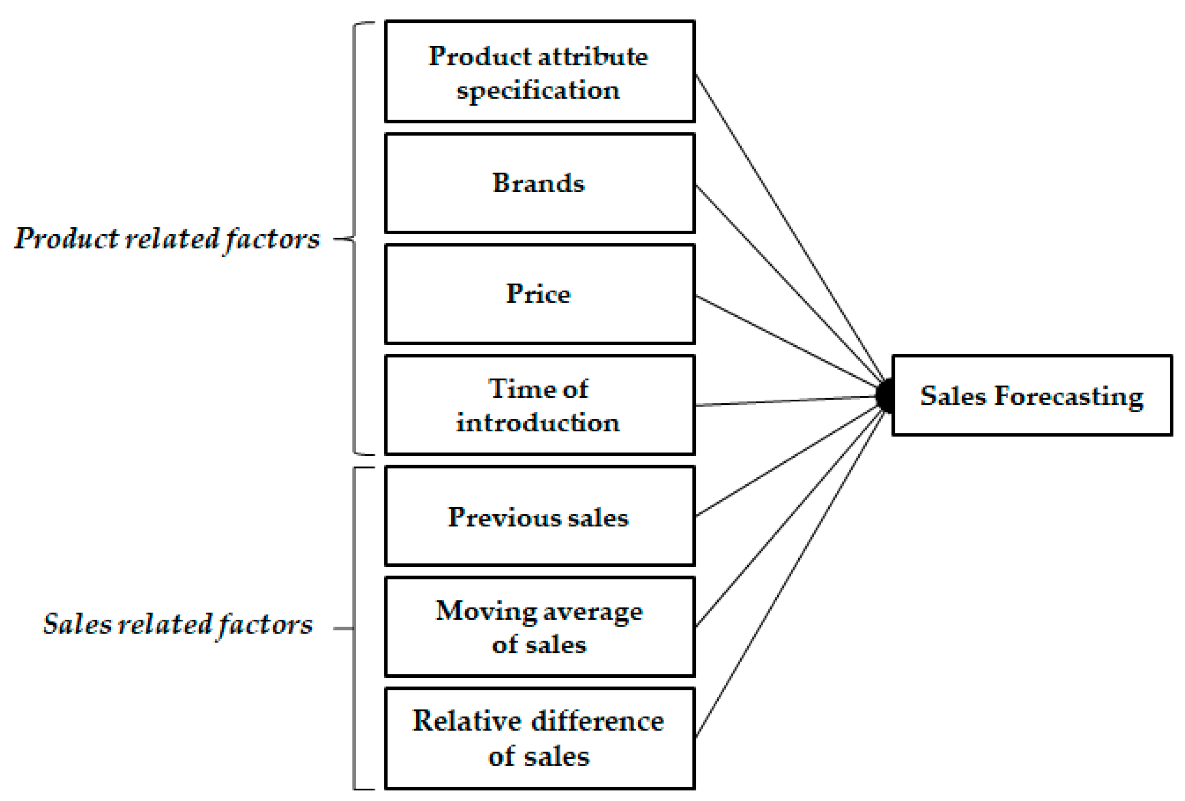
2.1. Sales Forecasting Related Factors

Figure 1 illustrates the conceptual model for integrated sales forecasting adopted in this study. Sales forecasting is influenced by a variety of factors, which can be categorized into product-related and sales-related factors.

2.1.1. Product Related Factors

• Product attribute specification: Product attribute specifications play a crucial role in shaping consumers’ perception of a product’s relevance to their personal needs. Understanding consumer preferences across different lifestyles is essential since individuals prioritize their functional and hedonic needs to varying extents [39]. For instance, when purchasing a tablet computer, customers consider factors such as the operating system, battery life, screen size, and RAM level. Therefore, it is reasonable to take into account attribute levels when forecasting sales [40]. In this study, we consider 14 attributes, including the operating system, display size (mm), display resolution (ppi), CPU processor speed (GHz), number of processor cores, rear camera pixels (MP), front camera pixels (MP), storage (GB), width (mm), length (mm), depth (mm), weight (g), battery capacity (mAh), and RAM (GB).
• Brands: Brand image plays a vital role in building brand equity, which encompasses consumers’ overall perception and emotional response towards a brand, influencing their behaviors. Marketers aim to shape consumers’ perceptions and attitudes towards a brand through marketing activities. The goal is to establish a strong brand image in consumers’ minds, stimulate their purchasing behavior, boost sales, maximize market share, and develop brand equity [41].
• Price: Price plays a significant role in consumer purchasing decisions and is equally important for providers [42]. Lower pricing can impact sales volume, as some providers strategically price certain products low to attract the attention of consumers with the intention of selling them other, higher-priced items. However, consumers may question the quality of a product if the price is excessively low. Many consumers prioritize value over the lowest price and are willing to pay a price that reflects the worth of a product. Setting prices too low can create a perception among consumers that a product is less satisfactory compared to similar products on the market [43].
• Time of Introduction: Products like mobile phones have short release cycles, making it crucial to consider this factor when forecasting sales. Continuous releases of new mobile phone models in the market create competition, trends, and consumer demand [4]. Technology products, including mobile phones, often experience high sales immediately after their release, followed by a rapid decline in the sales curve. Therefore, the time elapsed since the product release is a significant factor in understanding the sales pattern [44,45]. The value assigned to the months after release starts with 1 for the month of release and incrementally increases by 1 for each subsequent month.

2.1.2. Sales Related Factors

• Previous sales: In the manufacturing industry, the previous month’s sales have been identified as a particularly influential parameter in sales forecasting [6]. This suggests that the sales performance in the immediately preceding month plays a significant role in predicting future sales. Furthermore, research conducted in this domain has consistently shown that not only the previous month’s sales but also the sales figures from the two to three months prior can impact the sales outcomes in the predicted months [7,8].
• Moving average of sales: Capturing the trend of sales is recognized as a crucial variable in related studies. One commonly employed method to represent this trend is the use of moving averages. It is a prevalent research practice to calculate the moving average of sales over a period of two to three months [6,7]. By calculating the average sales over this time window, the moving average provides a smoothed representation of the sales trend, allowing for a better understanding and prediction of sales patterns.
• Relative difference of sales: The majority of time series data commonly demonstrate discernible vibration patterns that can either exhibit a decreasing or increasing trend. These patterns are quantified as relative difference variables, which represent the growth rates of sales over time. Such variables hold significant importance as primary factors within sales forecasting models [46,47].

Therefore, a total of 24 predictor variables, comprising both sales-related and product-related variables, are depicted in

Table 1. List of the predictor variables.

Variable	Description
X1	Display size (mm)
X2	Display resolution (ppi)
X3	Operate System
X4	CPU processor speed (GHz)
X5	Number of processor cores
X6	Rear camera pixels (MP)
X7	Front camera pixels (MP)
X8	RAM (GB)
X9	Storage (GB)
X10	Width (mm)
X11	Length (mm)
X12	Depth (mm)
X13	Weight (g)
X14	Battery capacity (mAh)
X15	Brand
X16	Release price (KRW)
X17	Time of introduction
X18	Previous 1 month’s sales
X19	Previous 2 month’s sales
X20	Previous 3 month’s sales
X21	Previous 1–2 month’s moving average of sales
X22	Previous 1–3 month’s moving average of sales
X23	Relative difference between the previous 1 month’s sales and the previous 2 month’s sales
X24	Relative difference between the previous 1 month’s sales and the previous 3 month’s sales

.

2.2. Machine Learning Methods

This section describes 12 machine learning models applied in our study.

2.2.1. Ridge, Lasso Regression

Multiple linear regression models tend to overfit. The relationship between feature values and label values was analyzed in more detail than necessary. This results in poor generalization and poor prediction of new data. Ridge and Lasso are methods used to overcome these shortcomings. The Ridge regression model is a method of estimating the regression coefficient by minimizing the objective function by adding an L2 penalty term to the sum of error squares in an existing regression expression [48]. The loss in Ridge regression is defined as:

$${Loss}_{ridge}\left(\widehat{\beta }\right)={\sum }_{i=1}^n{\left(y_i-x_i^{\prime }\widehat{\beta }\right)}^2+\lambda \sum _{j=1}^m{\beta }_j^2$$

(1)

where $\beta$ is the regression coefficient associated with the input parameters of the Ridge model; $x$ and $y$ are the input and output, respectively, $n$ is the number of samples in the training dataset, and the hyperparameter $\lambda$ is the penalty parameter.

The Lasso regression model is a method in which the L1 Penalty term is added [49]. The loss in Lasso regression is defined as:

$${Loss}_{lasso}\left(\widehat{\beta }\right)={\sum }_{i=1}^n{\left(y_i-x_i^{\prime }\widehat{\beta }\right)}^2+\lambda \sum _{j=1}^m\left|{\beta }_j\right|$$

(2)

where $x$ and $y$ are the input and output vector, respectively, $n$ is the number of samples in the training dataset, β is the regression coefficient, and λ is the penalty parameter.

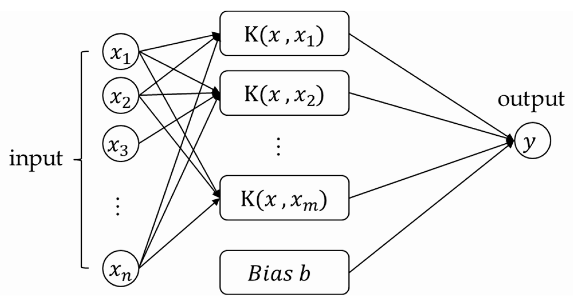
2.2.2. Support Vector Regression

Support Vector Machine (SVM) is a supervised learning model that solves computational problems that predict using a kernel. Specifically, the main objective of SVM is to create the best decision boundaries to separate n-dimensional spaces into separate classes. In SVM, the best decision boundary is called a hyperplane. The hyperplanes help improve the predictive power of the model and reduce errors in prediction and classification [50]. Figure 2 shows the main structure of the SVM. $y$ represents the model’s output, and b is the bias term to be optimized based on the regularized function. K is the kernel function. As shown in Figure 2, this is a small subset extracted from the training data by a related algorithm consisting of SVMs. Additionally, the kernel is used to transform the data into the necessary form through input. The SVM models use different types of kernel functions such as linear kernel, Bessel kernel, and radial basis kernel. The most popular of these kernel functions is the radial basis kernel with nonlinear characteristics.

2.2.3. Random Forest Regression

Random Forest (RF) is a tree-based ensemble model used to construct predictive models using objective functions as regression functions. The RF model uses data samples to create multiple decision trees, calculate each tree, and vote to produce the best results [51]. Key functions of the RF include speed and flexibility that generate the relationship between input and output functions. RF also handles large datasets more efficiently than other machine learning techniques.

2.2.4. Gradient Boosting Regression

Gradient Boosting Machine (GBM) is a tree-based ensemble model, learning several weak learners sequentially, learning the wrong residuals, updating weights and improving errors. In particular, the gradient descent method is used as a method of updating the weights. The process repeats unless the maximum number of trees is reached or the response is improved [52].

2.2.5. AdaBoost Regression

AdaBoost or Adaptive Boost is a tree-based ensemble model, which is a machine learning sequential ensemble technique used to randomly combine several weak learners in a dataset to create powerful learners. Among all training data sets, each sample observation is weighted, identifying false predictions and weighing them to further assign them to the next learner. The exact process repeats until the algorithm can correctly classify the output [53].

2.2.6. XGBoost Regression

XGBoost is a tree-based ensemble model that uses the Base Learner as the decision tree and learns in a way that compensates for the weaknesses of the previous model. Specifically, XGBoost uses a boosting algorithm to continuously correct fitting effects; each tree grows from the residuals of the previous tree and weights the ensemble output of all regression trees to obtain predictions [54].

2.2.7. Lightgbm Regression

Lightgbm is a tree-based ensemble model that uses leaf-based segmentation rather than tree-based segmentation. This creates a deep, asymmetric tree while continuously segmenting leaf nodes with maximum loss values without balancing the tree. This minimizes the prediction error loss compared to the tree-based segmentation scheme [55].

2.2.8. CatBoost Regression

CatBoost is a tree-based ensemble model created to solve the overfitting problem of existing boosting models. To this end, CatBoost learns after calculating the residual with only a part of the learning data, and as a result, the model is rebuilt [56].

2.2.9. Deep Neural Network

Deep Neural Network (DNN) is a machine learning and deep learning method that defines complex architectures for artificial neural networks (ANN). In ANN, artificial neurons (nodes) that form a network by combining synapses change the binding strength of synapses through learning, minimizing errors between predicted and actual values [57]. DNN is a learning method with two or more hidden layers in an ANN structure [58]. Figure 3 shows the main structure of the DNN with two layers. The $y$ represents the model’s output and $h$ is the neurons. In practice, neural networks with two hidden layers are widely used and have performed very well for time series data [59].

2.2.10. Recurrent Neural Network

Recurrent Neural Network (RNN) is a neural network-structured algorithm that is used for time-dependent or sequential data learning because it contains internal circulatory structures. It is an algorithm that can express information as previous information is accumulated in the current information by the internal circulation structure, and the information can be constantly updated because the data are circulated [60]. Given $x_t$ as an input, unit time $t$, its hidden state $h_t$. It is then computed as Equation (3):

$$h_t=\mathrm{t}\mathrm{a}\mathrm{n} h(W_h·\left[h_{t-1},x_t\right]+b_h)$$

(3)

where $W_h$ and $b_h$ are parameters to be learned and $\mathrm{t}\mathrm{a}\mathrm{n}h$ is a hyperbolic tangent function.

2.2.11. Long Short-Term Memory

Long Short-Term Memory (LSTM) is a neural network-structured algorithm designed to enable long/short-term memory by compensating for the shortcomings that existing RNNs cannot remember information far from the output. It is mainly used for time series prediction and natural language processing. To solve dependency and vanishing gradient problems, LSTM uses the cell state to adaptively adjust the amount of historical memory and the new information currently available [61]. LSTM comprises two state vectors: unit at time $t$, hidden state $h_t$ and cell state $C_t$, and three gates: forget gate $f_t$, input gate $i_t$, and output gate $o_t$. Each state and gate is computed as follows:

$$f_t=\sigma (W_f·\left[h_{t-1},x_t\right]+b_f)$$

(4)

$$i_t=\sigma (W_i·\left[h_{t-1},x_t\right]+b_i)$$

(5)

$$o_t=\sigma (W_o·\left[h_{t-1},x_t\right]+b_o)$$

(6)

$${\tilde{C}}_t=\mathrm{t}\mathrm{a}\mathrm{n}h(W_g\left[h_{t-1},x_t\right]+b_g)$$

(7)

$$C_t=f_t\times c_{t-1}+i_t\times g_t$$

(8)

$$h_t=o_t\times \mathrm{t}\mathrm{a}\mathrm{n}h\left(c_t\right)$$

(9)

where $W$ and $b$ are parameters to be learned and $\sigma$ is a sigmoid function as an activation function. The cell state ensures long-term dependence between data points in the input sequence and allows the LSTM to be applied to long sequence data.

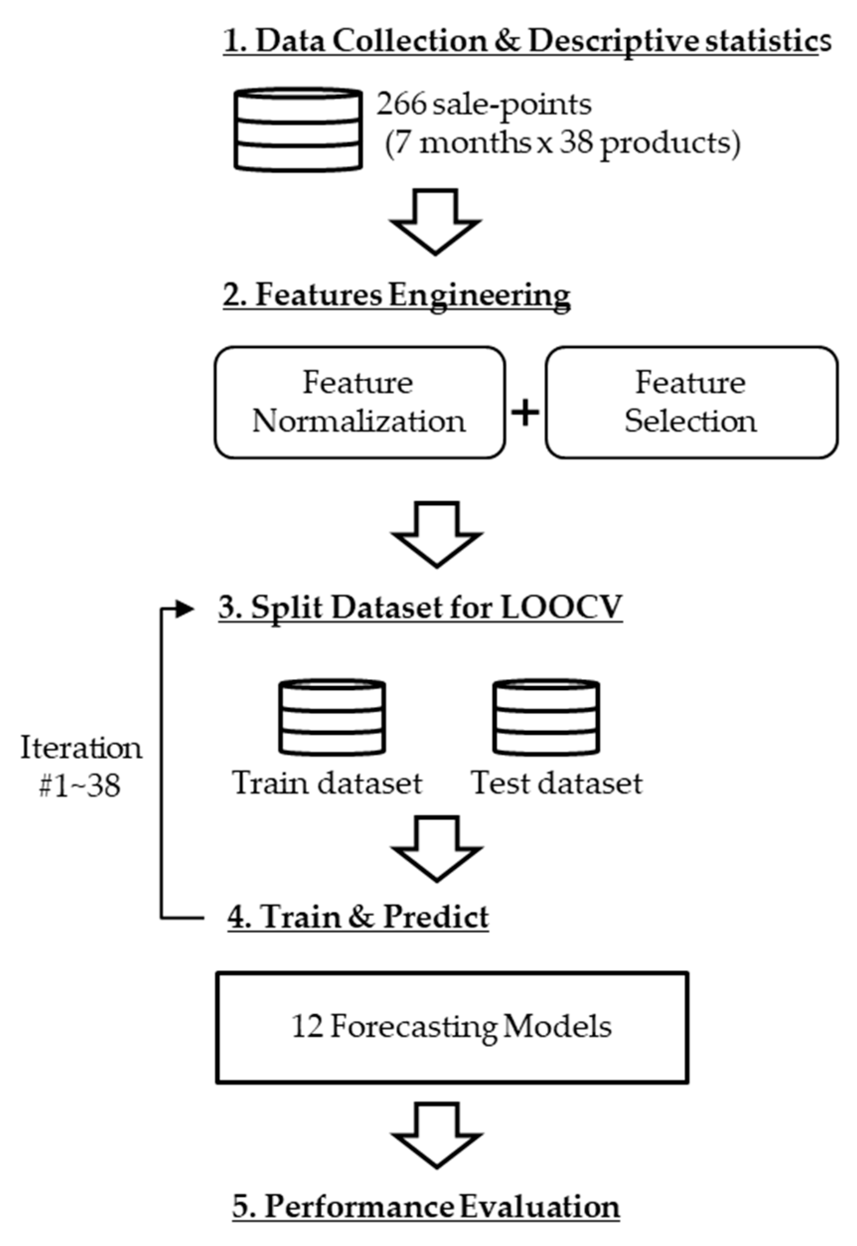
3. Experiments and Results

In this section, we present the experiments conducted and the results obtained from the performance comparison analysis of the forecasting models. The methodology is outlined in Figure 4. Initially, we collected the required data for analysis. Subsequently, descriptive statistics were examined for sales and other pertinent variables to enhance our comprehension of the dataset. Following this, we applied feature normalization and feature selection techniques to preprocess the data for modeling. These steps ensured the appropriate scaling of input features and the inclusion of only the most relevant ones in the analysis. Next, we employed the Leave-One-Out Cross-Validation (LOOCV) technique to forecast values for the test dataset to find robust models. Additionally, this approach is suitable as a sales forecasting scenario for cases where there is little sales data, such as short-term and newly released products. Finally, the MAPE, RMSE, and Correlation metrics compare the predicted value with the actual value to find the best-performing forecasting model.

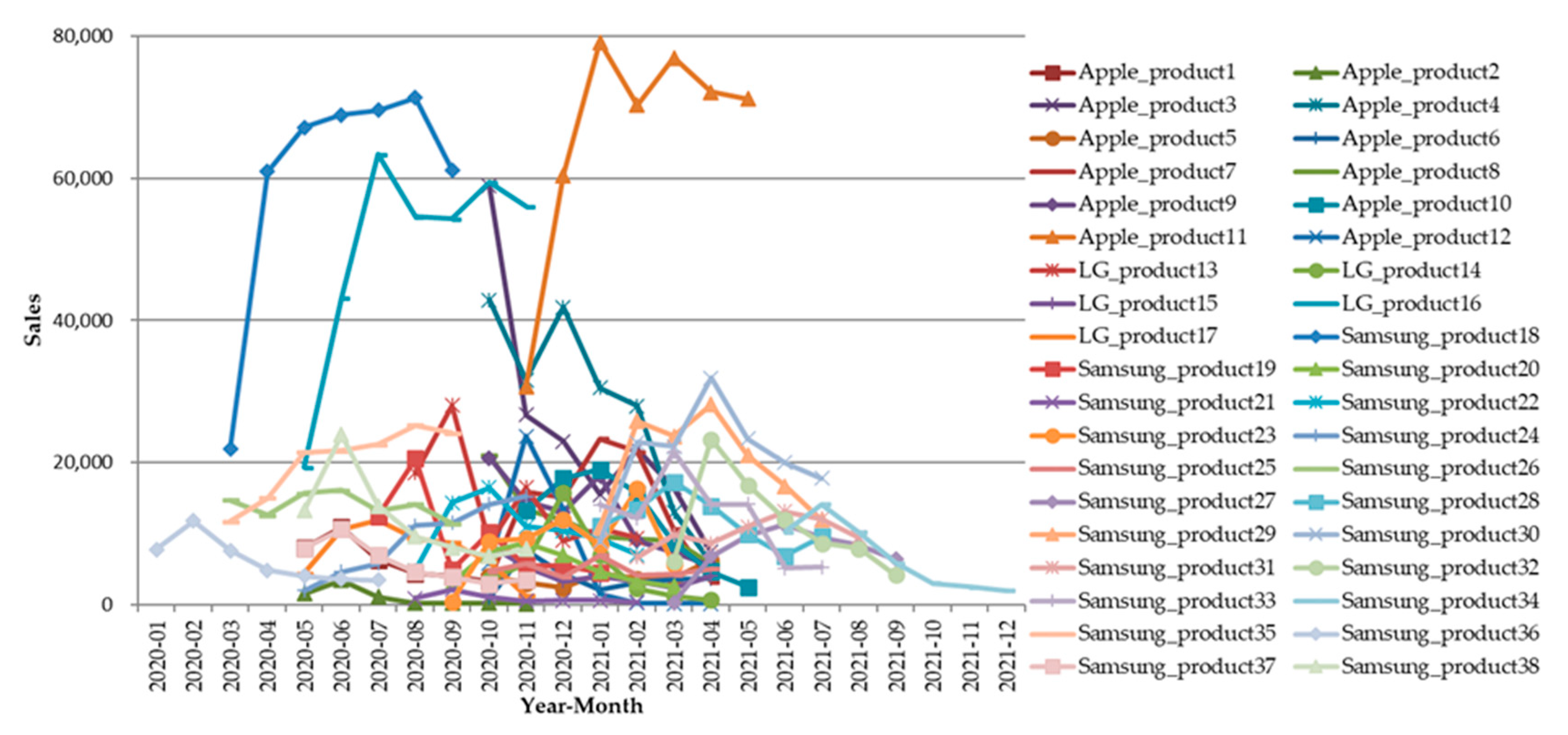
3.1. Data Collection and Descriptive Statistics

In this study, we collected sales data for 38 mobile phones from January 2020 to December 2021, specifically, the monthly sales data for 7 months after each mobile phone is released. The sales data used in this study are provided by one of the three telecommunication companies in South Korea and include the monthly sales data for each mobile product. Figure 5 illustrates the monthly sales trend for each mobile phone over the seven months following its release. The graph includes 38 products, categorized as 22 Samsung-branded, 12 Apple-branded, and 4 LG-branded products. Each line represents a specific product. Among the 38 mobile phones, five of them achieved monthly sales exceeding 40,000 units at least once during the observation period. On the other hand, the remaining thirty-three mobile phones had sales below this threshold. It is observed that the sales of mobile phones generally exhibit an initial increase in the first three months after their release. However, the growth rate gradually diminishes in the subsequent months. Additionally, we refrained from removing outliers through outlier analysis to avoid excluding relatively high-selling products. Additionally, since forecasting high-selling products is crucial, our model training includes sales datasets for all products. This comprehensive approach ensures that our predictions encompass the entire sales spectrum, including high-performing products. In addition to the sales data, we also gathered 14 product attribute specifications for each mobile phone. These specifications include details such as the brand and release price. The release price data were obtained from the well-known mobile phone information website “http://www.cetizen.co.kr” accessed on 3 April 2023. Additionally, 14 detailed specifications for each product were collected from the official websites of Samsung, LG, and Apple. The product specifications can be found on Samsung’s ‘https://www.samsung.com’ accessed on 3 April 2023, LG’s ‘https://www.lge.co.kr’ accessed on 3 April 2023, and Apple’s ‘https://www.apple.com’ accessed on 3 April 2023.

In

Table 2. Descriptive statistics of X, Y variables.

Variable	Characteristics	Mean	Std. Dev	Min	Max
Y	continuous	14,184.68	16,156.55	100	79,158
X1	continuous	160.78	15.91	96.6	192.7
X2	continuous	407.97	77.73	246	536
X3	discrete	-	-	-	-
X4	continuous	2.65	0.44	1.4	3.09
X5	continuous	7.14	1.28	4	8
X6	continuous	55.95	37.35	8	168
X7	continuous	15.43	9.21	5	40
X8	continuous	6.27	3.08	2	12
X9	continuous	160.86	102.34	32	512
X10	continuous	155.45	11.75	122	169.5
X11	continuous	74.3	9.87	60.2	128.2
X12	continuous	8.21	1.53	6.9	16.1
X13	continuous	187.32	31.06	133	282
X14	continuous	3751.14	1007.93	1812	5000
X15	discrete	-	-	-	-
X16	continuous	976,829.73	485,853.42	199,100	1,760,000
X17	continuous	4	2	1	7
X18	continuous	12,617.78	15,749.29	0	79,158
X19	continuous	10,752.53	14,984.32	0	79,158
X20	continuous	8721.73	13,868.59	0	79,158
X21	continuous	10,873.87	15,032.38	0	74,744.50
X22	continuous	8805.38	14,151.91	0	75,489.33
X23	continuous	−0.16	0.81	−7.92	0.96
X24	continuous	−0.16	0.87	−8.76	2.16

, we present the descriptive statistics of the X and Y variables used to forecast sales for the 38 mobile phones released in Korea between January 2020 and December 2021.

3.2. Feature Engineering

3.2.1. Feature Normalization

Improper data normalization can negatively impact the performance of both Machine Learning and Deep Learning models [62,63]. When variables possess varying magnitudes, machine learning techniques may fail to accurately capture their influence on the dependent variable. By applying the min–max scaling method, the normalization of values can effectively mitigate the impact of disparate magnitudes on the analysis results. This normalization process ensures a more reliable representation of the variable’s influence, regardless of their original scales.

$$x_{normalization }=\frac{x-x_{min}}{x_{max}-x_{min}}$$

(10)

3.2.2. Feature Selection

Feature selection is a valuable technique that reduces the number of features used in model building, resulting in a more concise model that is quick to train, analyze, and comprehend. To avoid subjective human intervention, many studies employ quantitative methods for feature selection. Random Forest is a commonly used method for this purpose, as demonstrated in several previous studies [64,65,66]. Typically, variables with feature importance close to zero are eliminated [64]. In our study, we also employed Random Forest for feature selection.

To analyze the feature importance using the Random Forest method, categorical variables such as brand and operating system were converted into dummy variables. Additionally, since the number of trees utilized affects the estimation of variable importance, we performed the analysis with various numbers of trees (200, 500, 1000, and 2000) to obtain robust results for variable importance [64]. The average value of feature importance was calculated based on these different tree configurations. As depicted in Figure 6, the analysis of feature importance led to the removal of variables with close to zero importance, such as brand, number of processor cores, and operating system. Previous 1–2 months’ moving average of sales, rear camera pixels, release price, and CPU processor speed were identified as variables of high importance. Consequently, the number of selected variables was reduced to 21.

3.3. Demand Forecasting Models

In this study, we define the 12 models listed below for sales forecasting:

(1).

Ridge regression;

(2).

Lasso regression;

(3).

Support vector regression with non-linear kernel;

(4).

Random forest regression;

(5).

Gradient boosting regression;

(6).

AdaBoost regression;

(7).

Lightgbm regression;

(8).

XGBoost regression;

(9).

CatBoost regression;

(10).

DNN with two hidden layers, Relu activation function and rmsprop optimizer;

(11).

RNN with two hidden layers, Relu activation function and rmsprop optimizer;

(12).

LSTM with two hidden layers, Relu activation function and rmsprop optimizer.

We utilized the 12 models mentioned above to compare their performance in sales forecasting. The key hyperparameter settings employed in this study are presented in

Table 3. Hyperparameters for our experiments.

Model	Hyperparameter	Candidate Values	Selected Value
Ridge	alpha	[0.1, 0.3, 0.5, 0.7, 0.9, 1, 3, 5]	1
Lasso	alpha	[0.1, 0.3, 0.5, 0.7, 0.9, 1, 3, 5]	0.7
SVM	cost	[1000, 2000, 3000, 4000, 5000]	3000
Random Forest	number of estimators	[100, 300, 500, 700, 900]	300
GBM	number of estimators	[100, 300, 500, 700, 900]	100
AdaBoost	number of estimators	[100, 300, 500, 700, 900]	300
Lightgbm	number of estimators	[100, 300, 500, 700, 900]	300
XGBoost	number of estimators	[100, 300, 500, 700, 900]	500
CatBoost	number of estimators	[100, 300, 500, 700, 900]	300
DNN	number of neurons	[16, 32, 64, 128]	64
RNN	number of neurons	[16, 32, 64, 128]	32
LSTM	number of neurons	[16, 32, 64, 128]	32

. The hyperparameter “alpha” corresponds to the regularization intensity for Lasso and Ridge, while the hyperparameter “cost” relates to SVM. For Random Forest, GBM, AdaBoost, LightGBM, XGBoost, and CatBoost, the hyperparameter “number of estimators” refers to the number of boosting trees. As for DNN, RNN, and LSTM, the hyperparameter represents the number of neurons. We set candidate values to find the optimal hyperparameters and selected the hyperparameters with the lowest RMSE and MAPE for the test dataset.

3.4. Performance Comparison of Models

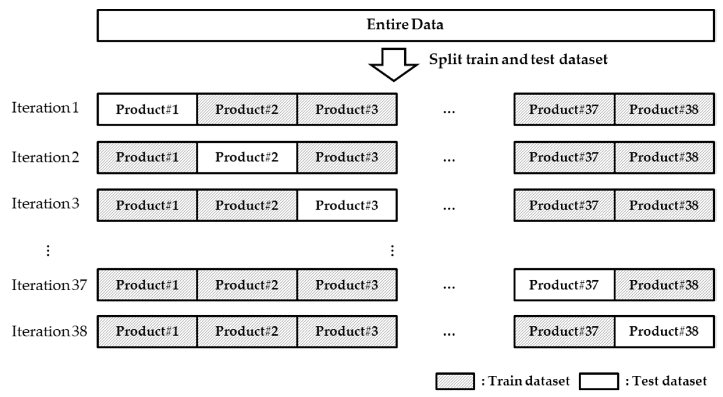
3.4.1. Leave-One-Out Cross Validation

To assess the forecasting performance and calculate the error rate of sales forecasting, we employed Leave-One-Out Cross-Validation (LOOCV) [67]. LOOCV involves training a model on all but one product and then evaluating the sales forecasting performance on the excluded product using the trained model. This process is repeated for all products in the dataset, ensuring comprehensive testing and minimizing randomness to obtain stable results. In our study, as illustrated in Figure 7, we conducted 38 iterations corresponding to the number of mobile phones and the error of the predicted values was computed. This approach is appropriate because it trains and predicts data from the same category of products when there is little sales data, such as short-term and newly released products.

3.4.2. Evaluation Metric

To evaluate the performance of the models, the evaluation metrics employed in this study include Mean Absolute Percentage Error (MAPE), Root Mean Square Error (RMSE), and Correlation. MAPE provides insights into the average absolute deviations in terms of percentages, making it a suitable indicator for detecting marginal errors. Conversely, RMSE, which relies on standard deviation, is particularly sensitive to values with significant errors or outliers [68].

$$\mathrm{M}\mathrm{A}\mathrm{P}\mathrm{E}=\frac{100}{n}\left|\frac{y_i-{\widehat{y}}_i}{y_i}\right|$$

(11)

$$\mathrm{R}\mathrm{M}\mathrm{S}\mathrm{E}=\sqrt{\sum _{i=1}^n\frac{{\left(y_i-{\widehat{y}}_i\right)}^2}{n} }$$

(12)

$n$ represents for the number of data indexes; $y_i$ and ${\widehat{y}}_i$ are considered as actual sales, and predicted sales.

Correlation is an indicator that analyzes the strength of the relationship between the predicted value and actual value.

$$\mathrm{C}\mathrm{o}\mathrm{r}\mathrm{r}\mathrm{e}\mathrm{l}\mathrm{a}\mathrm{t}\mathrm{i}\mathrm{o}\mathrm{n}=\frac{cov\left(y,{\widehat{y}}_{ }\right)}{{\sigma }_y{\sigma }_{{\widehat{y}}_{ }}}$$

(13)

where $cov$ is the covariance, ${\sigma }_y$ is the standard deviation of actual sales, and ${\sigma }_{{\widehat{y}}_{ }}$ is the standard deviation of predicted sales.

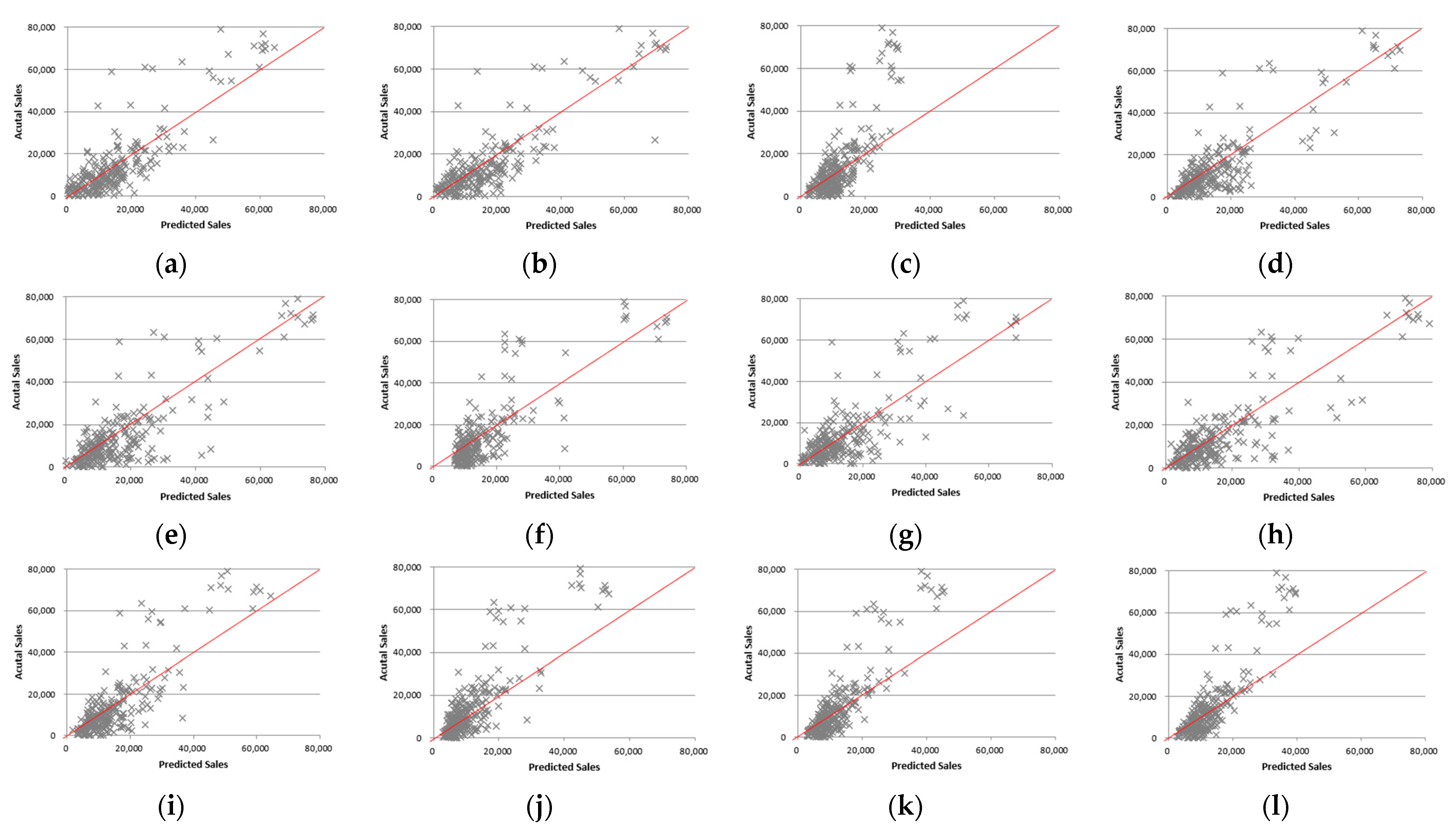
3.5. Predictive Performance

The scatterplot in Figure 8 depicts the relationship between actual sales and predicted sales for the test data using LOOCV. The plot includes 266 sale points, representing 7 months multiplied by 38 products. The purpose of this plot is to examine the correlation between predicted and actual sales. Ideally, a forecast that closely aligns with actual sales would follow the red line. Points below the red line indicate that predicted sales exceed actual sales, while points above the red line indicate the opposite. Based on Figure 8c, the Support Vector Model’s prediction reveals limitations in forecasting high-section sales. Additionally, the DNN, RNN, and LSTM models exhibit inaccuracies in predicting high-section sales. Specifically, these models tend to underestimate the actual values in the high sales range.

To gain deeper insights into the variations in predictive performance among the top three models, namely Random Forest, CatBoost, and AdaBoost, Figure 9 visually represents the actual sales and predicted sales generated by these models. It is evident from the figure that the Random Forest model outperformed the other two models across all sales ranges, demonstrating superior accuracy in sales forecasting.

3.6. Comparison of Models

After forecasting sales using 12 machine learning models, the results were compared and evaluated based on RMSE, MAPE, and Correlation. The total ranking was calculated by summing the rankings for each metric, with lower rankings indicating a more dominant model. A lower MAPE and RMSE corresponded to a higher ranking, while a larger Correlation also led to a higher ranking.

The evaluation of the test dataset was compared and analyzed using machine learning models, as presented in

Table 4. Performance results of sales forecasting models for test dataset.

Model	MAPE	RMSE	Correlation	Rank for MAPE	Rank for RMSE	Rank for Correlation	Total Ranking
Ridge	245.0623	9747.8058	0.8045	9	7	7	23
Lasso	116.9212	20,346.4701	0.5842	8	12	9	29
SVM	54.9216	12,307.4523	0.7904	6	8	8	21
Random Forest	42.6258	8443.3328	0.8629	1	1	1	3
GBM	54.8821	9643.082	0.8163	5	5	5	15
AdaBoost	46.5266	9354.7838	0.8285	3	4	3	10
Lightgbm	58.7273	9689.4442	0.8052	7	6	6	19
XGBoost	51.0913	9274.0941	0.8242	4	3	4	11
CatBoost	42.922	9201.2448	0.8434	2	2	2	6
DNN	293.7084	13,265.2662	0.4306	10	9	10	29
RNN	310.3341	13,835.2733	0.3706	11	10	11	32
LSTM	326.1333	15,673.6825	0.3229	12	11	12	35

. The Random Forest model demonstrated the best performance with an MAPE of 42.6258, RMSE of 8443.3328, and correlation of 0.8629. Conversely, the lowest-performing model was LSTM, with an MAPE of 326.1333, RMSE of 15,673.6825, and correlation of 0.3229. The Random Forest model consistently outperformed other models across all evaluation indicators. It exhibited performance similar to the second-place CatBoost model based on MAPE, showcased an error reduction rate of approximately 3.6% compared to the Ridge model based on RMSE, and achieved the highest correlation, with a slight 2.2% difference from the second-place CatBoost model.

We confirm that the Random Forest model exhibits the highest prediction performance as an integrated prediction model but further review the prediction accuracy according to the brand. As shown in

Table 5. Performance results for Random Forest forecasting models by brand.

Brand	MAPE	RMSE	Correlation
Samsung	35.2090	7075.6550	0.8952
Apple	47.83854	9665.8200	0.8634
LG	64.07153	40,535.66	0.3241

, all performance evaluation indicators showed high predictive performance in the order of Samsung brand products, Apple brand products, and LG brand products. To compare the forecasting accuracy between brands, based on Samsung brand products, Apple brand products had a relatively high error rate of 35.9%, RMSE, 36.6%, and a correlation of 3.5%, while LG brand products had a relative error rate of 82%, RMSE, 48.9%, and a correlation of 63.8%.

4. Conclusions

In the case of products with short-term lifecycles, such as mobile phones and new products, sales data collection is limited, making it difficult to predict sales. However, accurate sales forecasting is one of the important factors that maximize the company’s profits, so it is a problem to be solved. This study proposes an integrated model that trains product-related and sales-related variables that can understand sales patterns and product specifications for the same product category. To this end, the optimal model was identified and developed by comparing and evaluating the performance of 12 machine learning models using 38 mobile phone sales data in the Korean market between 2020 and 2021 to identify the best performance models. The following observations were found in the analysis of forecasting models considering product and sales-related variables:

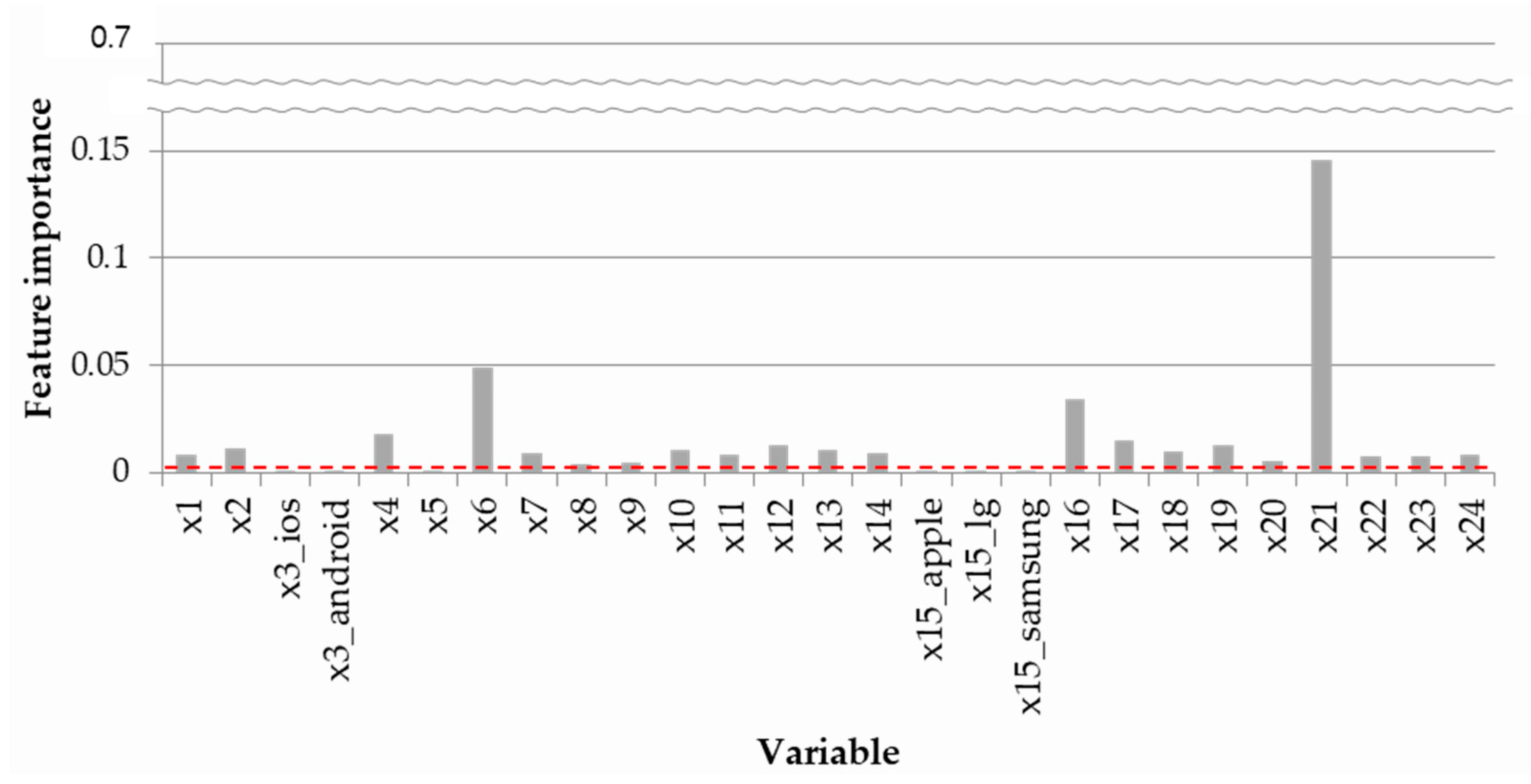
• For the mobile phone sales forecasting case, the previous 1–2 month’s moving average of sales for sales-related variables, and rear camera pixels, release price, and CPU processor speed for product-related variables were identified as variables that significantly affect sales.
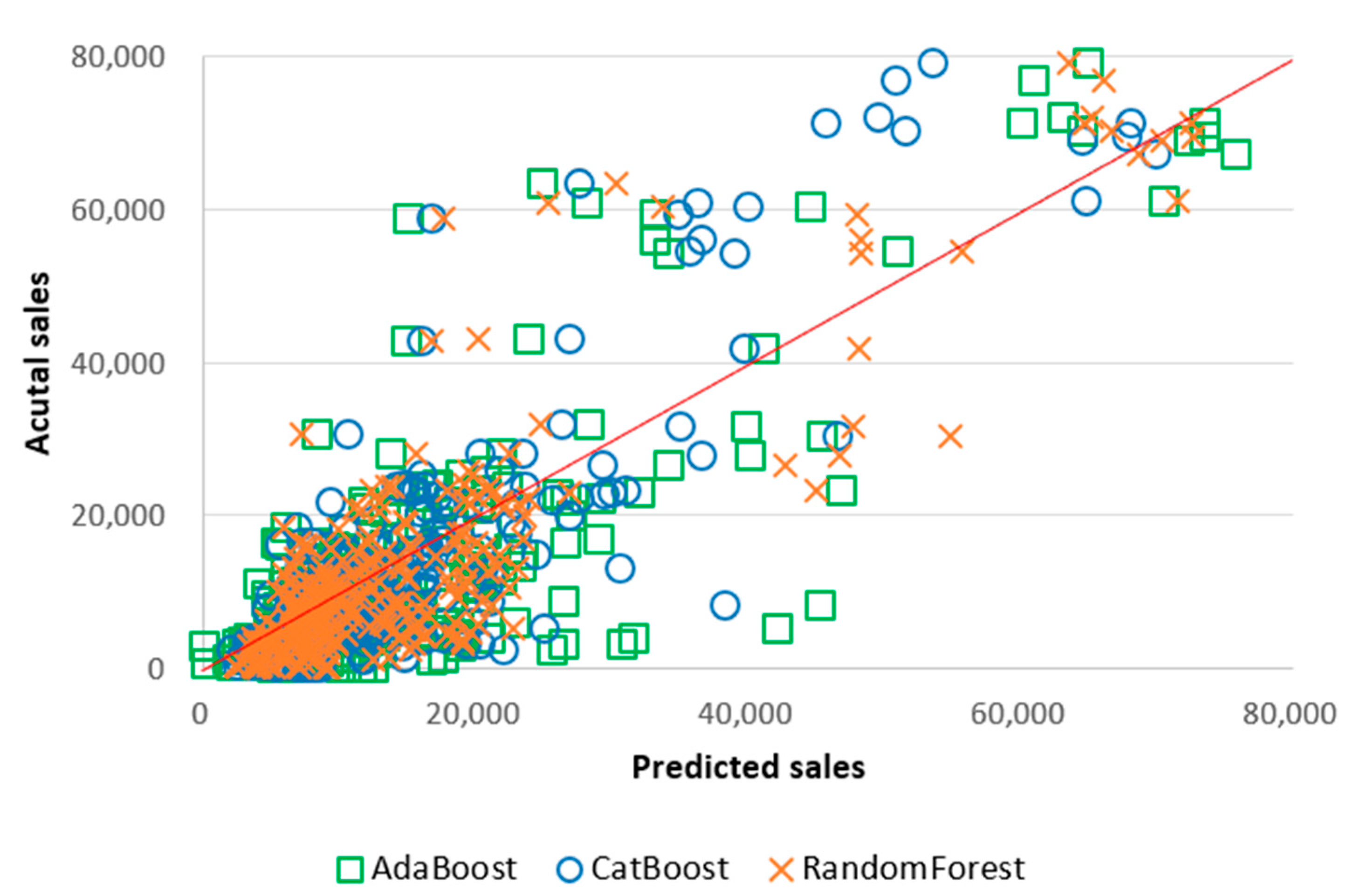
• The Random Forest model outperformed other models in sales forecasting, with the lowest-performing model, LSTM, exhibiting a significantly higher relative error percentage of 665% for MAPE and 86% for RMSE compared to Random Forest.
• The overall ranking order of the models, from best to worst performance, was as follows: Random Forest > CatBoost > AdaBoost > XGBoost > GBM > LightGBM > SVM > Ridge > Lasso > DNN > RNN > LSTM. Tree-based models (Random Forest, GBM, AdaBoost, LightGBM, XGBoost, CatBoost) outperformed neural network (DNN, RNN, LSTM) and linear (Ridge, Lasso) and SVM models.
• Consistent with previous studies [5], deep learning models such as DNN, RNN, and LSTM demonstrated lower performance than machine learning models when working with relatively small datasets.
• The Random Forest model, with the highest prediction performance, exhibited varying accuracy for each brand. The order of high accuracy was Samsung brand products > Apple brand products > LG brand products.

The analysis results of this study have the following important implications for companies engaged in sales forecasting of products with short lifecycles, such as mobile phones:

• Significant performance differences observed between the best and worst performance models highlight the need for informed decision making. Employing an unsuitable model can result in significant forecasting errors that accumulate over time, adversely impacting the entire supply chain. Thus, businesses should meticulously evaluate the specific characteristics of their sales data, consider the strengths and weaknesses of each model, and select the most suitable model aligned with their specific requirements and objectives.
• We believe that companies that produce short-term products can optimize the supply chain strategy by applying the Random Forest model or analysis process proposed by our study.
• The variation in predictive performance by brand may be attributed to differences in sales patterns resulting from brand-specific marketing strategies, including promotions and price policies [69,70]. To enhance forecasting accuracy, collecting additional data on promotion timing, price fluctuations, and advertising timing to reflect brand-specific marketing strategies would be beneficial.

Both directions to enhance model performance warrant further research. Firstly, assessing the impact of outlier processing on forecasting accuracy is crucial, as outliers can significantly influence results. Secondly, exploring the implementation of more advanced models, such as SGTM neural-like structures, modifications, and non-iterative approaches, holds promise for improving the overall forecasting performance. Furthermore, exploring the generalizability of our proposed forecasting approach is intriguing. A study report increased online sales of electronics during the COVID-19 pandemic [71], while others indicate a decrease in sales volume [72]. As research on the pandemic’s impact on sales is ongoing, analyzing our model’s predictive results before and after the COVID-19 pandemic could provide valuable insights to academia. This analysis would contribute to a better understanding of the model’s effectiveness under varying market conditions. Future research endeavors could focus on validating the findings in diverse markets, taking into account the unique characteristics of different product lifecycles. Additionally, conducting studies that involve the collection and analysis of daily or weekly sales data would contribute to a more comprehensive understanding of sales forecasting and should be a subject of interest for future investigations.

References

1. Fisher, M.; Rajaram, K. Accurate Retail Testing of Fashion Merchandise: Methodology and Application. Mark. Sci. 2000, 19, 266–278. [Google Scholar] [CrossRef]
2. Berg, J.M. Balancing on the Creative Highwire. Adm. Sci. Q. 2016, 61, 433–468. [Google Scholar] [CrossRef]
3. Lawrence, M.; Goodwin, P.; O’Connor, M.; Önkal, D. Judgmental Forecasting: A Review of Progress over the Last 25 years. Int. J. Forecast. 2006, 22, 493–518. [Google Scholar] [CrossRef] [Green Version]
4. Tsang, M.M.; Ho, S.-C.; Liang, T.-P. Consumer Attitudes toward Mobile Advertising: An Empirical Study. Int. J. Electron. Commer. 2004, 8, 65–78. [Google Scholar] [CrossRef]
5. Bailly, A.; Blanc, C.; Francis, É.; Guillotin, T.; Jamal, F.; Wakim, B.; Roy, P. Effects of Dataset Size and Interactions on the Prediction Performance of Logistic Regression and Deep Learning Models. Comput. Methods Programs Biomed. 2021, 213, 106504. [Google Scholar] [CrossRef]
6. Sharma, R.; Sinha, A.K. Sales Forecast of an Automobile Industry. Int. J. Comput. Appl. 2012, 53, 25–28. [Google Scholar] [CrossRef]
7. Lu, C.-J.; Lee, T.-S.; Lian, C.-M. Sales Forecasting for Computer Wholesalers: A Comparison of Multivariate Adaptive Regression Splines and Artificial Neural Networks. Decis. Support Syst. 2012, 54, 584–596. [Google Scholar] [CrossRef]
8. Luxhøj, J.T.; Riis, J.O.; Stensballe, B. A Hybrid Econometric—Neural Network Modeling Approach for Sales Forecasting. Int. J. Prod. Econ. 1996, 43, 175–192. [Google Scholar] [CrossRef]
9. Brühl, B.; Hülsmann, M.; Borscheid, D.; Friedrich, C.M.; Reith, D. A Sales Forecast Model for the German Automobile Market Based on Time Series Analysis and Data Mining Methods. In Advances in Data Mining, Proceedings of the Advances in Data Mining. Applications and Theoretical Aspects: 9th Industrial Conference, ICDM 2009, Leipzig, Germany, 20–22 July 2009; Springer: Berlin/Heidelberg, Germany, 2009; pp. 146–160. [Google Scholar] [CrossRef]
10. AlMamlook, R.E.; Kwayu, K.M.; Alkasisbeh, M.R.; Frefer, A.A. Comparison of Machine Learning Algorithms for Predicting Traffic Accident Severity. In Proceedings of the 2019 IEEE Jordan International Joint Conference on Electrical Engineering and Information Technology (JEEIT), Amman, Jordan, 9–11 April 2019. [Google Scholar] [CrossRef]
11. Liu, H.; Liu, Y.; Li, G.; Wen, L. Tourism Demand Nowcasting Using a LASSO-MIDAS Model. Int. J. Contemp. Hosp. Manag. 2021, 33, 1922–1949. [Google Scholar] [CrossRef]
12. Carbonneau, R.; Laframboise, K.; Vahidov, R. Application of Machine Learning Techniques for Supply Chain Demand Forecasting. Eur. J. Oper. Res. 2008, 184, 1140–1154. [Google Scholar] [CrossRef]
13. Güven, İ.; Şimşir, F. Demand Forecasting with Color Parameter in Retail Apparel Industry Using Artificial Neural Networks (ANN) and Support Vector Machines (SVM) Methods. Comput. Ind. Eng. 2020, 147, 106678. [Google Scholar] [CrossRef]
14. Hong, W.-C.; Dong, Y.; Chen, L.-Y.; Lai, C.-Y. Taiwanese 3G Mobile Phone Demand Forecasting by SVR with Hybrid Evolutionary Algorithms. Expert Syst. Appl. 2010, 37, 4452–4462. [Google Scholar] [CrossRef]
15. Xenochristou, M.; Hutton, C.; Hofman, J.; Kapelan, Z. Water Demand Forecasting Accuracy and Influencing Factors at Different Spatial Scales Using a Gradient Boosting Machine. Water Resour. Res. 2020, 56, e2019WR026304b. [Google Scholar] [CrossRef]
16. Hasan, R.; Kabir, M.A.; Shuvro, R.A.; Das, P. A Comparative Study on Forecasting of Retail Sales. arXiv 2022, arXiv:2203.06848. [Google Scholar] [CrossRef]
17. Henzel, J.; Sikora, M. Gradient Boosting Application in Forecasting of Performance Indicators Values for Measuring the Efficiency of Promotions in FMCG Retail. In Proceedings of the 2020 Federated Conference on Computer Science and Information Systems, Sofia, Bulgaria, 6–9 September 2020. [Google Scholar] [CrossRef]
18. Panarese, A.; Settanni, G.; Vitti, V.; Galiano, A. Developing and Preliminary Testing of a Machine Learning-Based Platform for Sales Forecasting Using a Gradient Boosting Approach. Appl. Sci. 2022, 12, 11054. [Google Scholar] [CrossRef]
19. Massaro, A.; Panarese, A.; Giannone, D.; Galiano, A. Augmented Data and XGBoost Improvement for Sales Forecasting in the Large-Scale Retail Sector. Appl. Sci. 2021, 11, 7793. [Google Scholar] [CrossRef]
20. Ul, I.; Nazir, K. Predicting Future Gold Rates Using Machine Learning Approach. Int. J. Adv. Comput. Sci. Appl. 2017, 8, 12. [Google Scholar] [CrossRef] [Green Version]
21. Osman AI, A.; Ahmed, A.N.; Chow, M.F.; Huang, Y.F.; El-Shafie, A. Extreme Gradient Boosting (Xgboost) Model to Predict the Groundwater Levels in Selangor Malaysia. Ain Shams Eng. J. 2021, 12, 1545–1556. [Google Scholar] [CrossRef]
22. Haselbeck, F.; Killinger, J.; Menrad, K.; Hannus, T.; Grimm, D.G. Machine Learning Outperforms Classical Forecasting on Horticultural Sales Predictions. Mach. Learn. Appl. 2021, 7, 100239. [Google Scholar] [CrossRef]
23. Labib, M.F.; Rifat, A.S.; Hossain, M.M.; Das, A.K.; Nawrine, F. Road Accident Analysis and Prediction of Accident Severity by Using Machine Learning in Bangladesh. In Proceedings of the 2019 7th international conference on smart computing & communications (ICSCC), Sarawak, Malaysia, 28–30 June 2019. [Google Scholar] [CrossRef]
24. Mitra, A.; Jain, A.; Kishore, A.; Kumar, P. A Comparative Study of Demand Forecasting Models for a Multi-Channel Retail Company: A Novel Hybrid Machine Learning Approach. In Operations Research Forum; Springer: Berlin/Heidelberg, Germany, 2022; Volume 3. [Google Scholar] [CrossRef]
25. Kaya, A.; Kaya, G.; Çebi, F. Forecasting Automobile Sales in Turkey with Artificial Neural Networks. Int. J. Bus. Anal. 2019, 6, 50–60. [Google Scholar] [CrossRef]
26. Ramyar, S.; Kianfar, F. Forecasting Crude Oil Prices: A Comparison between Artificial Neural Networks and Vector Autoregressive Models. Comput. Econ. 2017, 53, 743–761. [Google Scholar] [CrossRef]
27. Saha, P.; Gudheniya, N.; Mitra, R.; Das, D.; Narayana, S.; Tiwari, M.K. Demand Forecasting of a Multinational Retail Company Using Deep Learning Frameworks. IFAC-Pap. 2022, 55, 395–399. [Google Scholar] [CrossRef]
28. Bouktif, S.; Fiaz, A.; Ouni, A.; Serhani, M. Optimal Deep Learning LSTM Model for Electric Load Forecasting Using Feature Selection and Genetic Algorithm: Comparison with Machine Learning Approaches. Energies 2018, 11, 1636. [Google Scholar] [CrossRef] [Green Version]
29. Lorente-Leyva, L.L.; Alemany, M.; Peluffo-Ordóñez, D.H.; Araujo, R.A. Demand Forecasting for Textile Products Using Statistical Analysis and Machine Learning Algorithms. In Asian Conference on Intelligent Information and Database Systems; Springer: Berlin/Heidelberg, Germany, 2021; pp. 181–194. [Google Scholar] [CrossRef]
30. Seda Hatice, G.; Boran, S. Prediction of demand for red blood cells using ridge regression, artificial neural network, and integrated taguchi-artificial neural network approach. Int. J. Ind. Eng. 2022, 29, 1. [Google Scholar] [CrossRef]
31. Huang, J.; Chen, Q.; Yu, C. A New Feature Based Deep Attention Sales Forecasting Model for Enterprise Sustainable Development. Sustainability 2022, 14, 12224. [Google Scholar] [CrossRef]
32. Petroșanu, D.-M.; Pîrjan, A.; Căruţaşu, G.; Tăbușcă, A.; Zirra, D.-L.; Perju-Mitran, A. E-Commerce Sales Revenues Forecasting by Means of Dynamically Designing, Developing and Validating a Directed Acyclic Graph (DAG) Network for Deep Learning. Electronics 2022, 11, 2940. [Google Scholar] [CrossRef]
33. Schmidt, A.; Kabir, M.W.U.; Hoque, M.T. Machine Learning Based Restaurant Sales Forecasting. Mach. Learn. Knowl. Extr. 2022, 4, 105–130. [Google Scholar] [CrossRef]
34. Kim, M.; Lee, S.; Jeong, T. Time Series Prediction Methodology and Ensemble Model Using Real-World Data. Electronics 2023, 12, 2811. [Google Scholar] [CrossRef]
35. Tkachenko, R.; Izonin, I.; Vitynskyi, P.; Lotoshynska, N.; Pavlyuk, O. Development of the Non-Iterative Supervised Learning Predictor Based on the Ito Decomposition and SGTM Neural-Like Structure for Managing Medical Insurance Costs. Data 2018, 3, 46. [Google Scholar] [CrossRef] [Green Version]
36. Izonin, I.; Tkachenko, R.; Vitynskyi, P.; Zub, K.; Tkachenko, P.; Dronyuk, I. Stacking-Based GRNN-SGTM Ensemble Model for Prediction Tasks. In Proceedings of the 2020 International Conference on Decision Aid Sciences and Application (DASA), Sakheer, Bahrain, 8–9 November 2020. [Google Scholar] [CrossRef]
37. Tang, L.; Wu, Y.; Yu, L. A Non-Iterative Decomposition-Ensemble Learning Paradigm Using RVFL Network for Crude Oil Price Forecasting. Appl. Soft Comput. 2018, 70, 1097–1108. [Google Scholar] [CrossRef]
38. Tanaka, K. A Sales Forecasting Model for New-Released and Nonlinear Sales Trend Products. Expert Syst. Appl. 2010, 37, 7387–7393. [Google Scholar] [CrossRef]
39. Zhu, H.; Wang, Q.; Yan, L.; Wu, G. Are Consumers What They Consume?—Linking Lifestyle Segmentation to Product Attributes: An Exploratory Study of the Chinese Mobile Phone Market. J. Mark. Manag. 2009, 25, 295–314. [Google Scholar] [CrossRef]
40. Schneider, M.J.; Gupta, S. Forecasting Sales of New and Existing Products Using Consumer Reviews: A Random Projections Approach. Int. J. Forecast. 2016, 32, 243–256. [Google Scholar] [CrossRef]
41. Zhang, Y. The Impact of Brand Image on Consumer Behavior: A Literature Review. Open J. Bus. Manag. 2015, 3, 58–62. [Google Scholar] [CrossRef] [Green Version]
42. Walters, R.G. Assessing the Impact of Retail Price Promotions on Product Substitution, Complementary Purchase, and Interstore Sales Displacement. J. Mark. 1991, 55, 17–28. [Google Scholar] [CrossRef]
43. Keefer, A. How Does Poor Pricing Affect the Success of a Product? Available online: https://smallbusiness.chron.com/poor-pricing-affect-success-product-36373.html (accessed on 28 March 2023).
44. Burmester, A.B.; Becker, J.U.; van Heerde, H.J.; Clement, M. The Impact of Pre- and Post-Launch Publicity and Advertising on New Product Sales. Int. J. Res. Mark. 2015, 32, 408–417. [Google Scholar] [CrossRef]
45. Tellis, G.J.; Stremersch, S.; Yin, E. The International Takeoff of New Products: The Role of Economics, Culture, and Country Innovativeness. Mark. Sci. 2003, 22, 188–208. [Google Scholar] [CrossRef] [Green Version]
46. Huarng, K.; Yu, T.H.-K. Ratio-Based Lengths of Intervals to Improve Fuzzy Time Series Forecasting. IEEE Trans. Syst. Man Cybern. Part B 2006, 36, 328–340. [Google Scholar] [CrossRef]
47. Lu, C.-J. Sales Forecasting of Computer Products Based on Variable Selection Scheme and Support Vector Regression. Neurocomputing 2014, 128, 491–499. [Google Scholar] [CrossRef]
48. Marquardt, D.W.; Snee, R.D. Ridge Regression in Practice. Am. Stat. 1975, 29, 3. [Google Scholar] [CrossRef]
49. Tibshirani, R. Regression Shrinkage and Selection via the Lasso: A Retrospective. J. R. Stat. Soc. Ser. B 2011, 73, 273–282. [Google Scholar] [CrossRef]
50. Boser, B.E.; Guyon, I.M.; Vapnik, V.N. A Training Algorithm for Optimal Margin Classifiers. In Proceedings of the Fifth Annual Workshop on Computational Learning Theory—COLT ’92, Pittsburgh, PA, USA, 27–29 July 1992. [Google Scholar] [CrossRef] [Green Version]
51. Breiman, L. Random Forests. Mach. Learn. 2001, 45, 5–32. [Google Scholar] [CrossRef] [Green Version]
52. Friedman, J.H. Greedy Function Approximation: A Gradient Boosting Machine. Ann. Stat. 2001, 29, 1189–1232. [Google Scholar] [CrossRef]
53. Freund, Y.; Schapire, R. A Short Introduction to Boosting. J. Jpn. Soc. Artif. Intell. 1999, 14, 771–780. [Google Scholar]
54. Chen, T.; Guestrin, C. XGBoost: A Scalable Tree Boosting System. In Proceedings of the 22nd ACM SIGKDD International Conference on Knowledge Discovery and Data Mining—KDD ’16, San Francisco, CA, USA, 13–17 August 2016; pp. 785–794. [Google Scholar] [CrossRef] [Green Version]
55. Ke, G.; Meng, Q.; Finley, T.; Wang, T.; Chen, W.; Ma, W.; Ye, Q.; Liu, T.-Y. LightGBM: A Highly Efficient Gradient Boosting Decision Tree. Adv. Neural Inf. Process Syst. 2017, 30, 3149–3157. [Google Scholar]
56. Prokhorenkova, L.; Gusev, G.; Vorobev, A.; Dorogush, A.V.; Gulin, A. CatBoost: Unbiased Boosting with Categorical Features. Neural Information Processing Systems. Available online: https://proceedings.neurips.cc/paper/2018/hash/14491b756b3a51daac41c24863285549-Abstract.html (accessed on 15 April 2023).
57. Jain, A.K.; Mao, J.; Mohiuddin, K.M. Artificial Neural Networks: A Tutorial. Computer 1996, 29, 31–44. [Google Scholar] [CrossRef] [Green Version]
58. Schmidhuber, J. Deep Learning in Neural Networks: An Overview. Neural Netw. 2015, 61, 85–117. [Google Scholar] [CrossRef] [Green Version]
59. Kaastra, I.; Boyd, M. Designing a Neural Network for Forecasting Financial and Economic Time Series. Neurocomputing 1996, 10, 215–236. [Google Scholar] [CrossRef]
60. Medsker, L.; Jain, L.C. Recurrent Neural Networks: Design and Applications; CRC Press: Boca Raton, FL, USA, 1999. [Google Scholar]
61. Hochreiter, S.; Schmidhuber, J. Long Short-Term Memory. Neural Comput. 1997, 9, 1735–1780. [Google Scholar] [CrossRef] [PubMed]
62. Passalis, N.; Tefas, A.; Kanniainen, J.; Gabbouj, M.; Iosifidis, A. Deep Adaptive Input Normalization for Time Series Forecasting. IEEE Trans. Neural Netw. Learn. Syst. 2020, 31, 3760–3765. [Google Scholar] [CrossRef] [PubMed] [Green Version]
63. Ambarwari, A.; Jafar Adrian, Q.; Herdiyeni, Y. Analysis of the Effect of Data Scaling on the Performance of the Machine Learning Algorithm for Plant Identification. J. RESTI 2020, 4, 117–122. [Google Scholar] [CrossRef]
64. Genuer, R.; Poggi, J.-M.; Tuleau-Malot, C. Variable Selection Using Random Forests. Pattern Recognit. Lett. 2010, 31, 2225–2236. [Google Scholar] [CrossRef] [Green Version]
65. Kursa, M.B.; Rudnicki, W.R. The All Relevant Feature Selection using Random Forest. arXiv 2011, arXiv:1106.5112. [Google Scholar] [CrossRef]
66. Behnamian, A.; Millard, K.; Banks, S.N.; White, L.; Richardson, M.; Pasher, J. A Systematic Approach for Variable Selection with Random Forests: Achieving Stable Variable Importance Values. IEEE Geosci. Remote Sens. Lett. 2017, 14, 1988–1992. [Google Scholar] [CrossRef] [Green Version]
67. Wong, T.-T. Performance Evaluation of Classification Algorithms by K-Fold and Leave-One-out Cross Validation. Pattern Recognit. 2015, 48, 2839–2846. [Google Scholar] [CrossRef]
68. Chai, T.; Draxler, R.R. Root Mean Square Error (RMSE) or Mean Absolute Error (MAE)?—Arguments against Avoiding RMSE in the Literature. Geosci. Model Dev. 2014, 7, 1247–1250. [Google Scholar] [CrossRef] [Green Version]
69. Ehrenberg, A.S.C.; Hammond, K.; Goodhart, G.J. The After-Effects of Price-Related Consumer Promotions. J. Advert. Res. 1994, 34, 11–22. [Google Scholar]
70. Jee, T.W. The Perception of Discount Sales Promotions—A Utilitarian and Hedonic Perspective. J. Retail. Consum. Serv. 2021, 63, 102745. [Google Scholar] [CrossRef]
71. Valaskova, K.; Durana, P.; Adamko, P. Changes in Consumers’ Purchase Patterns as a Consequence of the COVID-19 Pandemic. Mathematics 2021, 9, 1788. [Google Scholar] [CrossRef]
72. Rossolov, A.; Aloshynskyi, Y.; Lobashov, O. How COVID-19 Has Influenced the Purchase Patterns of Young Adults in Developed and Developing Economies: Factor Analysis of Shopping Behavior Roots. Sustainability 2022, 14, 941. [Google Scholar] [CrossRef]
Figure 1. A conceptual framework of integrated sales forecasting for mobile phones.
Electronics 12 03256 g001
Figure 2. Main structure of Support Vector Machine.
Electronics 12 03256 g002
Figure 3. Main structure of Deep Neural Network with two layers.
Electronics 12 03256 g003
Figure 4. Process for comparison performance analysis of the forecasting models.
Electronics 12 03256 g004
Figure 5. Monthly Sales of each mobile phone.
Electronics 12 03256 g005
Figure 6. Variable importance for mobile phone sales.
Electronics 12 03256 g006
Figure 7. Train and test datasets for product-specific LOOCV validation.
Electronics 12 03256 g007
Figure 8. Actual versus predicted sales of mobile phone using (a) Ridge regression, (b) Lasso regression, (c) Support Vector regression, (d) Random Forest regression, (e) Gradient boosting regression, (f) AdaBoost regression, (g) Lightgbm regression, (h) XGboost regression, (i) Catboost regression, (j) DNN, (k) RNN and (l) LSTM.
Electronics 12 03256 g008
Figure 9. Scatter plot of measured sales and predicted sales with Random Forest, CatBoost, AdaBoost.
Electronics 12 03256 g009