Skeleton-Based Human Action Recognition Based on Single Path One-Shot Neural Architecture Search

Abstract

Skeleton-based human action recognition based on Neural Architecture Search (NAS.) adopts a one-shot NAS strategy. It improves the speed of evaluating candidate models in the search space through weight sharing, which has attracted significant attention. However, directly applying the one-shot NAS method for skeleton recognition requires training a super-net with a large search space that traverses various combinations of model parameters, which often leads to overly large network models and high computational costs. In addition, when training this super-net, the one-shot NAS needs to traverse the entire search space of the complete skeleton recognition task. Furthermore, the traditional method does not consider the optimization of the search strategy. As a result, a significant amount of search time is required to obtain a better skeleton recognition network model. A more efficient weighting model, a NAS skeleton recognition model based on the Single Path One-shot (SNAS-GCN) strategy, is proposed to address the above challenges. First, to reduce the model search space, a simplified four-category search space is introduced to replace the mainstream multi-category search space. Second, to improve the model search efficiency, a single-path one-shot approach is introduced, through which the model randomly samples one architecture at each step of the search training optimization. Finally, an adaptive Covariance Matrix Adaptation Evolution Strategy (CMA-ES) is proposed to obtain a candidate structure of the perfect model automatically. With these three steps, the entire network architecture of the recognition model (and its weights) is fully and equally trained significantly. The search and training costs will be greatly reduced. The search-out model is trained by the NTU-RGB + D and Kinetics datasets to evaluate the performance of the proposed model’s search strategy. The experimental results show that the search time of the proposed method in this paper is 0.3 times longer than that of the state-of-the-art method. Meanwhile, the recognition accuracy is roughly comparable compared to that of the SOTA NAS-GCN method.

1. Introduction

Skeleton-based human action recognition has grown in popularity as a research topic in computer vision in recent years. It has been extensively employed in various domains, including human–computer interaction and stage performance arts. A Graph Convolutional Network (GCN) [1,2] is the mainstream method for skeleton recognition, which excels in handling non-Euclidean data and has produced outstanding outcomes in human skeleton recognition. However, when creating a 10-layer network that alternates between a spatial GCN and temporal GCN, it is typically necessary to use a GCN for the skeletal recognition directly. To find the perfect network layout and training settings, and to achieve an adequate recognition accuracy, a significant amount of manual training and intricate ablation experiments are frequently needed. Some researchers have suggested using the GCN and the NAS (Neural Architecture Search) to automatically determine the best network layout and parameters to increase the model’s recognition effectiveness. For instance, the literature (Pérez-Rúa, Juan-Manuel et al.) [3] proposed a multi-modal skeleton recognition model based on neural architecture search, which achieved a high recognition accuracy in the skeleton recognition task. However, to introduce NAS into the skeleton recognition task, factors such as the number of layers of the skeleton recognition model, the selection of the optimization modules in the model, and the categories and weights of the dataset need to be considered. As a result, NAS should initially offer a vast search space for the skeleton identification operation. The optimal model parameters, however, take a while to converge because there are too many candidate operations in the search space.

Training thousands of models is difficult or impossible for a traditional machine learning task. To solve the problem of architecture search for models, the researchers propose the idea of sharing weights between models: instead of the traditional method of training thousands of individual models from scratch, a super network is proposed, which can be trained to simulate any architecture in the search space. To make the search more flexible, instead of deciding whether a particular layer is convolutional, average pooling, or maximum pooling, the method changes the search space to mix all of the above choices in one search process. The search time is reduced by assigning weights to each component of the search space when training the skeleton model (Peng, Wei et al., 2020) [4]. A simple example of a search space is shown in Figure 1, where one can apply a 3 × 3 convolution, 5 × 5 convolution, or max-pooling layer at specific locations in the network. The search space contains three different operations; the one-shot model adds their outputs together. The implementation idea is to treat all operations, such as convolution, average pooling, and maximum pooling, as channels and allow the controller to select a mask over these channels. It is possible to train a single model containing all three operations, rather than training three separate models. By allowing the parameters to be shared between all the architectures in the search space, thus avoiding the need to train each architecture from scratch, it is more computationally efficient than a standard NAS.

However, the weight-sharing method based on NAS must traverse the whole network’s search space, which causes the search process to be overtrained in the NAS search area, and results in the absence of optimization and an automated optimization strategy. Therefore, the NAS has to thoroughly search the ideal network topology and training parameters for the skeleton identification challenge. This thesis considers the field of a GCN based on a Single Path One-Shot Neural Architecture Search (SNAS-GCN) for human skeleton recognition as the main subject of its study. In this paper, a simplified, four-category NAS search space for skeleton recognition tasks is proposed. Subsequently, to reduce the search training time of the super-net and obtain an excellent skeleton recognition model in a relatively short period, the weight-sharing search is replaced by a single path random search, which is a single path one-shot search strategy. Applying SNAS-GCN to the skeletal identification job is not simple. Skeleton recognition jobs have complicated and bloated search spaces due to the different types of models (RNN, CNN, and GCN) and data inputs (skeleton data and RGB data). A challenging problem in this domain is optimizing the search process in the NAS space. In addition, many combinations of network layers and parameters are applied to the skeleton recognition task. Obtaining the optimal combination and optimal network structure using an optimization-seeking algorithm is another challenge. To quickly identify the ideal neural network in the search space, the Covariance Matrix Adaptation Evolution Strategy (CMA-ES) is presented. With the proposed SNAS-GCN strategy, a graph convolutional network for skeleton recognition is constructed rapidly. In evaluating the performance of the search strategy proposed in this paper, the model approach took 18 h less than the NAS-GCN model to train a skeleton recognition network with a roughly comparable accuracy on the NTU-RGB + D [5] and Kinetics [6] datasets.

The contributions of this paper include the following two points:

• To improve the search efficiency and reduce the NAS search time, the optimization operation of the NAS search space is simplified. Secondly, a single-path one-shot weight-sharing model is proposed to replace the original weight-sharing strategy.
• To automatically sample candidate networks from the super-net, a new covariance matrix adaptation evolution strategy is employed.

2. Related Work

2.1. Skeleton Recognition Based on GCN

Human action recognition based on skeleton data has attracted more attention due to its robustness to changes in human scale, viewpoint, and background. With the development of deep learning, traditional methods use recurrent neural networks (RNN) [5,7,8] and convolutional neural networks (CNN) [9,10,11,12] to compute and analyze skeleton data. However, the method based on RNNs and CNNs has a high complexity, and the model’s ability to deal with the skeleton structure needs to be improved [13]. A graph convolution network (GCN) can better capture the space–time relationship between bodies and extract the advanced features of the human skeleton. Therefore, in recent years, researchers have proposed a skeleton recognition model based on a graph convolution network (GCN). (Yan, Sijie, 2018) [1] proposed the spatiotemporal graph convolutional network (ST-GCN) model, which extracts human body feature information by introducing the Spatio-temporal map convolution network and solving the problem of the previous model only being able to deal with temporal features, but not extract spatial features. (Shi et al., 2019) proposed a two-stream adaptive graph convolutional network (2s-AGCN) [2] model based on the ST-GCN model, which improves performance by collecting the dual information of joints and bones. (Liu, Ziyu et al., 2020) [14] proposed an MS-G3D model based on multi-scale expansion. By eliminating the dependence between distances, it can directly model cross Spatio-temporal joints, which solves the problem of the previous methods not being able to capture complex Spatio-temporal relationships.

The above methods all adopt the skeleton recognition model based on a GCN. Although the GCN model has achieved good advantages in processing non-Euclidean data, implementing an efficient neural network usually requires the manual setting of the network parameters and a long training time. (Peng, Wei et al., 2020) [4] proposed the GCN-NAS model based on neural architecture search. The shortcoming of the previous GCN model only setting parameters manually is solved by introducing a neural architecture search of a dynamic graph. The limitation of the previously fixed graph is broken and the accuracy of the skeleton recognition is improved. By building an automatic search strategy for neural architectures, this paper hopes to solve the problem of the amount of time one needs to spend designing models for skeleton recognition networks.

2.2. Neural Architecture Search

Because neural architecture search can automatically find the optimal network model, this method provides a new possibility to avoid manually designing the network structure in the field of image vision [15,16,17,18,19]. For example, NAS algorithms based on reinforcement learning (RL) (Zoph, Barret, 2016) [19] can replace manually designed networks. However, such methods need to consume hundreds of GPUs for their search training. To reduce the search training time of traditional NAS methods, researchers have proposed a one-shot neural architecture search strategy [20]. For example, Brock et al. (2017) [15] proposed a SMASH model based on one-shot neural architecture search, which generates suboptimal weights by introducing an auxiliary network. The overall search speed is improved because the generated suboptimal weights are related to the weights of normal training in accuracy. In addition, (Pham et al., 2018) [18] proposed a neural structure search (ENAS) method based on sub-model weight sharing, which finds the neural network structure by introducing a controller to search the optimal sub-network in an ample search space. (Luo et al., 2018) [21] proposed an automatic neural network design method based on continuous optimization based on ENAS. This method maps the neural architecture to a constant vector space and solves the problems that could not be optimized in the continuous space in the past. (Zhu, Hui et al., 2019) [22] also proposed the EENAS method based on ENAS, which accelerates the search process by introducing a pre-learning strategy, thereby reducing the amount of computation. (Chu, Xiangxiang. 2021) [23] presented a uniformly sampled FairNAS technique, whose sampling and training procedures may completely use the search space’s potential and deliver the best results among similar one-off models. (Liang, Tingting et al., 2021) [24] proposed a new search space in which each candidate is closely connected by a directed acyclic graph. Therefore, the effective method has been excellent and the method’s mobility has been dramatically improved compared to the previous methods, and advanced results can be obtained on multiple datasets. In addition, this method proposes an efficient one-shot search algorithm to find the optimal path structure.

The above methods are all one-shot neural architecture search methods based on super-nets. This class of methods must first train a super-net and then use evolutionary algorithms to find the optimal candidate paths. However, the super-net needs to design a complex search space, which leads to a too-large network model and a long search training time. To quickly find the optimal neural network under the framework of one-shot neural architecture search, Guo [25] proposed a single-path sampling strategy to train the super network, which solves the problem of the search space of the previous model being too complex, and further reduces the search training time. (Bender et al., 2018) [26] introduced the dropout strategy, which solves the problem of the previous super network being too complicated by randomly deleting operations with low weights in the training process.

2.3. Graph Convolutional Networks Based on Neural Architecture Search

With the rapid development of neural architecture search, the time required for the automatic design of a graph neural network is significantly reduced. Recently, (Gao, Yang et al., 2020) [27] proposed a GraphNAS model based on neural architecture search and designed the best graph neural architecture by introducing reinforcement learning strategies. Furthermore, by introducing a novel parameter-sharing strategy in (Zhou, Kaixiong et al.) [28], an automatic graph neural network (AGNN) framework is proposed. The above methods show the possibility of applying neural architecture search to a graph neural network. However, due to the overly complex design of the search space, the search efficiency of traditional graph neural networks needs to be further optimized. To further improve the search efficiency of neural architecture search in the field of GCNs, (Ding, Yuhui et al., 2021) [29] proposed a differentiable search DiffMG model, which solves this problem by introducing a novel and efficient search algorithm. (CAI, Shaofei et al., 2021) [30] proposed a graph neural structure (GNAS) based on a gradient search strategy to obtain a higher performance. (Li, Guohao et al.) [31] proposed a greedy algorithm SGAS based on neural structure search, which can find the best architecture and reduce the search cost.

Inspired by the above research work, to improve the efficiency of neural architecture search and better apply it to the automatic search of a skeleton recognition model, this work designs a simplified search space and proposes a covariance adaptive improvement strategy based on an evolutionary algorithm to find the best architecture.

3. Methods

In this section, the single-path one-shot NAS-strategy-based methods for optimizing the GCN structure for skeleton recognition are proposed. First, the GCN-based skeleton recognition task is described in Section 3.1. Then, the one-shot single-path NAS strategy is described in Section 3.2. Next, the search space for the neural architecture search is defined in Section 3.3. Finally, Section 3.4 introduces how to automatically optimize the best GCN network from all the candidate architectures using the covariance matrix adaptive evolutionary algorithm (CMA-ES).

The framework of the SNAS-GCN is shown in Figure 2. Three functional modules are abstracted based on the graph neural architecture search process. The search space module contains a predefined search space for the GCN architecture, which can be customized by the user for a specific task. The GCN module is then used in the search space to implement the GCN model building and training for different downstream graph tasks on known graph data and configuration parameters. The search module implements the search function and search management for the GCN architecture, using a search algorithm to sample the GCN architecture for the best structure.

3.1. GCN-Based Skeleton Recognition Network

Motion capture devices or posture estimation techniques in a video can be used to gather skeleton data. Typically, these data consist of many frames. The joint coordinates that make up each frame of the data are included. As a result, the two-dimensional or three-dimensional coordinates of the human joints in each frame serve as typical representations of the skeleton sequence. An undirected spatiotemporal graph $\mathcal{G}=\{\mathcal{V},\mathcal{E},\mathcal{A}\}$ is built using a skeleton sequence in this study. The nodes and edges of this spatiotemporal graph represent the skeleton’s joints and bones, respectively, where $\mathcal{V}$ represents all the joints in the skeleton sequence and $\left|\mathcal{E}\right|$ represents the edge connection. An adjacency matrix ${\mathcal{A}\in \mathcal{R}}^{\mathcal{n}\times \mathcal{n}}$ represents the connection of the joints.

Spatial graph convolution and temporal graph convolution are the two main components of the spatio-temporal graph based on the skeleton recognition model. An example of a constructed spatio-temporal skeleton diagram, including spatial and temporal dimensions, is shown in Figure 3, where the joints are represented as vertices and their natural connections in the body are represented as spatial edges. For the temporal dimension, the corresponding joints between two adjacent frames are connected to temporal edges. Among these, one-dimensional convolution modeling is used in the temporal domain, while graph convolution modeling is used in the spatial domain. The model constructs a spatial–temporal map of the skeletal sequence in two steps. First, the joints within a frame are connected to the edges according to the connectivity of the human body structure. Second, in each frame, each joint will be connected to the same joint. The connections in this setting are naturally defined and do not need to be manually assigned. A supervised learning problem using graph data may be used to frame the skeletal recognition issue. The robust representation of $\mathbb{G}$ will be learned using a GCN to improve the action class prediction. The GCN model is built by using neural structure search, which automatically improves the skeletal recognition model.

The research inserts 10 GCN blocks into the network for the search and training to be compatible with existing state-of-the-art GCN approaches, as illustrated in Figure 4. The spatial module for each GCN block comprises channel convolution filters, which are convolution filters with a kernel size of 9 × 1 that are applied along the temporal axis to record temporal data. The graph is projected onto a feature space with channel 64 by the network’s initial GCN block. The outputs of three GCN layers with 64-dimensional channels follow. The output channels of the three layers are then multiplied by two to obtain a total of 128 dimensions. The finished three-layer network includes 256 output channels for different dimensions. Each GCN block is subjected to the ResNet technique, similar to (Yan, and Xong, 2018) [1]. The collected characteristics are then used to make a final prediction in a fully linked layer.

3.2. A Single Path One-Shot NAS Method

3.2.1. One-Shot Weight Sharing Method

Without a loss of generality, the architecture search space $\mathcal{A}$ is represented by a directed acyclic graph (D.A.G.). The network architecture is $\mathcal{a}\in \mathcal{A}$, denoted as $\mathcal{N}(\mathcal{a},\mathcal{w})$, with a weight $\mathcal{w}$.

The neural architecture search aims to solve two related problems. The first one is weight optimization, as shown in Equation (1):

$${\mathcal{w}}_{\mathcal{a}}=\underset{\mathcal{w}}{\mathrm{a}\mathrm{r}\mathrm{g}\mathrm{m}\mathrm{i}\mathrm{n}}{\mathcal{L}}_{\mathrm{t}\mathrm{r}\mathrm{a}\mathrm{i}\mathrm{n}}\left(\mathcal{N}\left(\mathcal{a},\mathcal{w}\right)\right)$$

(1)

where ${\mathcal{L}}_{\mathrm{t}\mathrm{r}\mathrm{a}\mathrm{i}\mathrm{n}}(·)$ is the loss function on the training set.

The second is architecture optimization. It finds architectures trained on the training set and has the best accuracy on the validation set, as shown in Equation (2):

$$\mathcal{a}*=\underset{\mathcal{a}\in \mathcal{A}}{\mathrm{a}\mathrm{r}\mathrm{g}\mathrm{m}\mathrm{a}\mathrm{x}}{\mathrm{A}.\mathrm{C}.\mathrm{C}.}_{\mathrm{v}\mathrm{a}\mathrm{l}}\left(\mathcal{N}\left(\mathcal{a},{\mathcal{w}}_{\mathcal{a}}\right)\right)$$

(2)

where $AC{C}_{\mathrm{v}\mathrm{a}\mathrm{l}}(·)$ is the accuracy of the validation set.

Traditional NAS methods perform these two optimization problems in a nested fashion. Many architectures are sampled from the $\mathcal{A}$ system and trained from scratch, as shown in Equation (1). The cost of each training is high, and only a small dataset and small search space (such as a single block) can complete this training in a short time.

To alleviate the above problems, the NAS method adopts a weight-sharing strategy. The architectural search space $\mathcal{A}$ is encoded in the super-net, denoted as $\mathcal{N}(\mathcal{A},\mathcal{W})$, where $\mathcal{W}$ is the weight in the super-net. The super-net is trained only once. The weights are directly inherited by all the architectures from $\mathcal{W}$. Therefore, they share weights in common graph nodes. The architecture can be fine-tuned as needed, but it does not need to be trained from scratch. This is achieved by dividing the training and architecture search of the super network into two consecutive steps. Therefore, the architecture search speed is improved.

In general, the formula for these two consecutive steps of the super-net is as follows: First, the weights of the super-net are optimized, as shown in Equation (3):

$$W_{\mathcal{A}}=\underset{W}{\mathrm{a}\mathrm{r}\mathrm{g}\mathrm{m}\mathrm{i}\mathrm{n}}{\mathcal{L}}_{\mathrm{t}\mathrm{r}\mathrm{a}\mathrm{i}\mathrm{n}}\left(\mathcal{N}\left(\mathcal{A},W\right)\right)$$

(3)

Second, the search architecture of the super-net is optimized, as shown in Equation (4):

$$\mathcal{a}*=\underset{\mathcal{a}\in \mathcal{A}}{\mathrm{a}\mathrm{r}\mathrm{g}\mathrm{m}\mathrm{a}\mathrm{x}}{\mathrm{A}.\mathrm{C}.\mathrm{C}.}_{\mathrm{v}\mathrm{a}\mathrm{l}}\left(\mathcal{N}\left(\mathcal{a},W_{\mathcal{A}}\left(\mathcal{a}\right)\right)\right)$$

(4)

During the search process, each sampled architecture $\mathcal{a}$ inherits its weights from $W_{\mathcal{A}}$ to $W_{\mathcal{A}}\left(\mathcal{a}\right)$. The main differences between Equations (1), (2) and (4) are that the architecture weights have been trained in advance, and the evaluation of $AC{C}_{\mathrm{v}\mathrm{a}\mathrm{l}}(·)$ only requires inference and does not need to retrain new Weights. Generally, the one-shot weight-sharing method is essentially one-shot training and multiple inferences. Therefore, the search efficiency is improved.

However, compared to traditional methods, the super network reduces the cost of the architecture search by an order of magnitude, but still needs to train a large enough super network. The super network should contain enough search space, resulting in a too-large network model, which increases the calculation cost, and the search efficiency still needs to be improved.

Recent one-shot approaches have attempted to use a “path dropout” strategy to address the problem of oversized super-network models [26]. Each edge in the super-net graph is randomly eliminated in Equation (3), and the dropout rate parameter controls the randomness. In the above way, the joint adaptation of the node weights is reduced during the training, thereby reducing the search time [32]. The dropout rate parameter, however, significantly impacts this strategy’s training methodology. Because of this, the issue of super-net training is challenging and still not fully resolved.

3.2.2. Single Path One-Shot Algorithm

The single path one-shot technique is introduced by revisiting the basic idea behind the concept of weight sharing. The effectiveness of the architectural search in Equation (4) critically depends on the fact that the inherited weights $W_{\mathcal{A}}\left(\mathcal{a}\right)$ do not require fine-tuning. Second, $W_{\mathcal{A}}\left(\mathcal{a}\right)$ can correctly forecast the architecture on the validation set. The weights $W_{\mathcal{A}}\left(\mathcal{a}\right)$ should, ideally, be close to the ideal weights ${\mathcal{w}}_{\mathcal{a}}$ in (1). The value of the approximation depends on how much the training loss ${\mathcal{L}}_{\mathcal{t}\mathcal{r}\mathcal{a}\mathcal{i}\mathcal{n}}\left(\mathcal{N}\right(\mathcal{a},W_{\mathcal{A}}\left(\mathcal{a}\right)\left)\right)$ is minimized, which demands that the weights $W_{\mathcal{A}}$ of the super-net be improved in a way that simultaneously improves all of the designs in the search space, as demonstrated in Equation (5):

$$W_{\mathcal{A}}=\underset{W}{\mathrm{a}\mathrm{r}\mathrm{g}\mathrm{m}\mathrm{i}\mathrm{n}}{\mathbb{E}}_{a\sim \mathsf{\Gamma }\left(\mathcal{A}\right)}\left[{\mathcal{L}}_{\mathrm{t}\mathrm{r}\mathrm{a}\mathrm{i}\mathrm{n}}\left(\mathcal{N}\left(\mathcal{a},W\left(\mathcal{a}\right)\right)\right)\right]$$

(5)

where $\mathsf{\Gamma }\left(\mathcal{A}\right)$ is the prior distribution of $\mathcal{a}\in \mathcal{A}$ during the training process. (Guo, Zichao et al.) [25] found that a uniformly constrained sampling method can better extract the ideal architectures from the search space. Equation (3) is realized explicitly in Equation (5). Thus, just one weight $W\left(\mathcal{a}\right)$ is enabled and updated at a time throughout each optimization phase while an architecture $\mathcal{a}$ is randomly selected. Memory use is effective, and being embodied as a random super-net, the super-net is no longer effective.

A single path super-net structure is proposed to reduce the cooperative adaptation between the node weights and achieve fast search results. Each architecture is a path, as shown in Figure 5. As the choice block does not recognize branches, a random path must be kept in this case. Therefore, by randomly selecting a sub-network, its validation accuracy is evaluated during the training phase.

As shown in Figure 5, the choice block is made up of several candidate structure alternatives. In Section 3.3, the choice block in the search space is described in detail as consisting of a Chebyshev choice block and feature structure choice block. In a single-path super-net, each choice block is executed one option at a time. By sampling every option block, a single path may be found.

The simplicity of this method is used to find different architectural elements by defining several choice blocks. To facilitate complex search spaces, two additional choice blocks are particularly recommended.

3.3. GCN Search Space Design

Designing a search space for single-path one-shot architecture search is a challenging problem, because the following competing requirements must be balanced. First, the search space should be reasonably designed and expressive enough to capture a variety of helpful candidate architectures. Secondly, the accuracy of the validation set generated by the one-shot model must be able to predict the accuracy generated by the independent model training. Finally, the one-shot model must be small enough to use limited computing resources (i.e., memory and time) for the search training [33].

To enrich the search space, this paper designs two choice blocks: the Chebyshev choice block and the feature structure choice block, as shown in Figure 6.

Figure 6a shows the Chebyshev choice block module, composed of a first- and second-order Chebyshev polynomial function. Figure 6b shows the characteristic structural choice block module. It consists of a spatial feature neural operation (spatial m), a temporal feature neural operation (temporal m), and a spatio temporal feature neural operation (spatio temporal m). The entire search space consists of a number of the two aforementioned choice blocks, which are sampled by a single path to search for a better skeleton recognition network.

3.3.1. Feature Structure Choice Blocks

As shown in Figure 3, human actions can be recognized and resolved through the temporal and spatial sequences of human joint positions. By forming a high-level representation of the skeletal sequence through the spatio-temporal map, the recognition efficiency and accuracy can be further improved. Thus, the feature structure choice block includes spatial feature neural operations, temporal feature neural operations, and spatio-temporal feature neural operations.

The spatial features are extracted based on the structural correlation of the spatial node connections. To determine the connection strength between two nodes, (Shi. 2019) [2] applied the normalized Gaussian function on the graph nodes and calculated the similarity score as the correlation of the nodes, as shown in Equation (6):

$$\forall i,j\in \mathcal{V},A_D\left(i,j\right)=\frac{e^{\varphi \left(h\left(x_i\right)\right)\otimes \psi \left(h\left(x_j\right)\right)}}{{\sum }_{j=1}^n{e}^{\varphi \left(h\left(x_i\right)\right)\otimes \psi \left(h\left(x_j\right)\right)}}$$

(6)

According to the $h\left(x_i\right)$ and $h\left(x_j\right)$ of the nodes and their corresponding representations, the correlation score $A_D\left(i,j\right)$ between them is calculated. $\varphi (\cdot )$ and $\psi (\cdot )$ are two projection functions, called $conv\_s$ in Figure 7, which can be implemented by channel convolution filters. This way, the correlation between the nodes can be captured, which is the spatial feature “Spatial m” in Figure 7.

The topology of the spatial feature map is the most intuitive. However, when temporal correlations are ignored, hidden joint connections are lost. For example, if there is no time information in the NTU-RGB + D dataset, it is difficult to tell whether a person is touching his head or waving his hand. As a result, including temporal information in action recognition models improves their accuracy. First, using Equation (6), the temporal feature introduces a Gaussian function, which calculates the node correlation. Second, to extract information from the temporal of each node, the functions $\varphi (\cdot )$ and $\psi (\cdot )$ are implemented by two temporal convolutions $conv\_t$, as shown in Figure 7. “Temporal m” is the name of this module.

Previous GCN approaches have been based on predefined graph structures constrained by temporal and spatial structures, while lacking a discussion of spatio-temporal correlations, thus ignoring the implied joint associations. However, different layers contain different semantic information, and therefore layer-specific mechanisms should be designed to construct a spatio-temporal graph.

The Spatio-temporal module, which is denoted as “Spatio-Temporal m” in Figure 7, can be directly constructed using “Spatial m” and “Temporal m.” After the spatial feature neural operations and temporal feature neural operations have been formulated, the Spatio-temporal feature neural operations within the skeleton sequence must be modelled. Through constructing the graph, the temporal dimension of the graph is built by connecting the identical joints, and the graph is constructed by connecting the similar joints in consecutive frames, which allows us to define a very simple strategy for extending the spatial graph into the spatio-temporal domain. The same Gaussian function sampling is required to complete the convolution operation on the spatio-temporal graph, as in the spatial-only or time-only cases. In this way, a good convolution operation is performed on the constructed spatio-temporal graph.

3.3.2. Chebyshev Choice Block

Chebyshev polynomials provide high-order connections to GCN networks and can obtain high-level graph features. Therefore, (Deferrard et al.) [34] introduced a new spectral domain graph convolution network, which accomplishes quick localization and a low complexity, to overcome the shortcomings of the early spectral domain graph convolution network. The convolution kernel ${\mathcal{g}}_{\mathsf{\theta }}$ in a spectral domain graph can be approximated by Chebyshev polynomials of order R, as shown in Equation (7):

$$Y={\sum }_{r=0}^R{\theta }_r^{\prime }{T}_r\left(\hat{L}\right)X$$

(7)

where $R=1{,\theta }_r^{\prime }$ denotes the Chebyshev coefficient. ${\mathrm{X}\in \mathcal{R}}^{\mathcal{n}}$ is the input representation of $\mathcal{G}$ and its $n$ elements. The Chebyshev polynomial $T_r\left(\hat{L}\right)$ is defined recursively as Equation (8):

$$T_r\left(\hat{L}\right)=2\hat{L}{T}_{r-1}\left(\hat{L}\right)-T_{r-2}\left(\hat{L}\right)$$

(8)

where, $T_0=1$ and $T_1=\hat{L}$. Here, $\hat{L}=2L/{\lambda }_{max}-I_n$ is normalized to [−1, 1], ${\lambda }_{max}=2$. The graph Laplacian $L$, of which the normalized definition is $L=I_n-D^{-1/2}A{D}^{-1/2}$ and $D_{ii}=\sum _j{A}_{ij}$, is used for Fourier transform. Chebyshev polynomial functions of the first or second order are constructed on different network layers in the search space, as shown in Figure 6. With a maximum order of 2, the function module can be built from Equation (8).

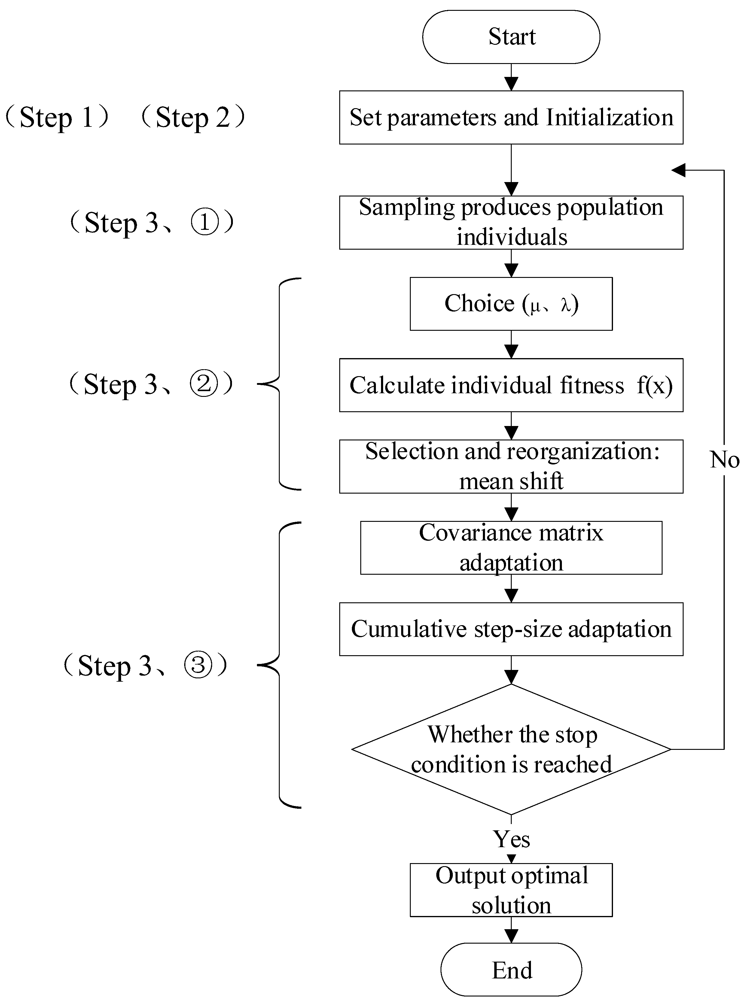
3.4. Search Strategy Algorithm

Random search for the architecture search in Equation (4) is adopted in the traditional search strategy algorithm. However, this has a limited effect on tight search spaces. This paper uses an evolutionary algorithm. The Covariance Matrix Adaptive Evolutionary Strategies (CMA-ES) is one of the most powerful evolutionary algorithms in the field of real-valued optimization, with many successful applications [35,36,37]. The invariance of CMA-ES, which is attained by carefully thought-out mutation and selection operators, and its successful adaptability to the mutation distribution, are its key benefits. The architectural parameter $\mathcal{a}$ is described by a Gaussian distribution in the CMA-ES method. Then, to update the distribution of architectures, the CMA-ES algorithm examines a collection of designs and chooses significant samples based on their performance. From the architectural dispersion, the optimal architecture can eventually be found.

The CMA-ES algorithm is divided into three parts, as shown in Figure 8.

Step 1: Parameter setting

This includes the number of children $\mathsf{\lambda }$, the number of parents $\mathsf{\mu }$, the recombination weight $w_i=1\dots \mathsf{\mu }$, the cumulative learning rate ${\mathcal{c}}_{\mathsf{\sigma }}$ controlled by the step size, the decay parameter ${\mathcal{d}}_{\mathsf{\sigma }}$ of the step size update, the cumulative learning rate ${\mathcal{c}}_{\mathcal{c}}$ of the rank-one update of the covariance matrix, the covariance matrix, the learning rate ${\mathcal{c}}_1$ of the variance matrix rank-one update, and the learning rate ${\mathcal{c}}_{\mathrm{u}}$ of the covariance matrix rank $\mathsf{\mu }$ update.

Step 2: Initialization

This includes choosing the distribution mean and step size. The evolutionary path is set as${:p}_{\sigma }=0,p_c=0$. The covariance matrix is set as $C=I$ and the number of current iterations is $\mathcal{g}=0$.

Step 3: Loop until the termination condition is reached

This includes ① sampling from the population, ② a reselection and recombination of the samples based on their fitness, and ③ updating the internal state variables based on the reordered samples.

This section describes, in detail, steps ② and ③ of step 3 above. Then, in the step of selecting reorganization, the new mean value of the search distribution is selected from the sample μ, the weighted average value of the points, through which the recombination of the best offspring is achieved to calculate the new parental status, as shown in Equations (9) and (10):

$$\begin{array}{cc}⟨\mathit{y}{⟩}_{\mathrm{w}}& ={\displaystyle \sum _{i=1}^{\mu }}{w}_i{\mathit{y}}_{i:\lambda }\hspace{1em}\hspace{1em}where\hspace{1em}\hspace{1em}{\displaystyle \sum _{i=1}^{\mu }}{w}_i=1,w_i>0\end{array}$$

(9)

$$\begin{array}{cc}\mathit{m}& \leftarrow \mathit{m}+\sigma ⟨\mathit{y}{⟩}_{\mathrm{w}}={\displaystyle \sum _{i=1}^{\mu }}{w}_i{\mathit{x}}_{i:\lambda }\end{array}$$

(10)

where $\mathit{m}$ is the mean and $\mu \le \lambda$ is the parent population size, i.e., the number of selected samples. ${\mathcal{w}}_{\mathcal{i}=1\dots \mu }\in \mathcal{R}+$: the positive weight coefficient for recombination, e.g., ${\mathcal{w}}_{\mathcal{i}=1\dots \mu }=1/\mu$. Equation (10) is equivalent to calculating the mean of $\mu$ selection points.

The fitness $f\left(\mathit{x}\right)$ is calculated for each new individual, as shown in Equation (11). The reselection and reorganization are performed according to the fitness.

$$f\left({\mathit{x}}_{1:\lambda }\right)\le f\left({\mathit{x}}_{2:\lambda }\right)\le \cdots \le f\left({\mathit{x}}_{i:\lambda }\right)$$

(11)

where ${\mathit{x}}_{i:\lambda }$: is the $i$-th optimal individual. According to the fitness ranking, the top $\mu <\lambda$ individuals are intercepted for parameter updating.

An evolutionary path is the sequence of consecutive steps taken over many generations for the update process in step 3, ③. A series of consecutive sums of steps can be used to represent an evolutionary path, and these sums are referred to as cumulative sums. Exponential smoothing is used to create the evolutionary path ${\mathit{p}}_{\mathrm{c}}$, and ${{\mathit{p}}_c}^{\left(0\right)}=0$, as seen in Equation (12):

$$\begin{array}{cc}{\mathit{p}}_{\mathrm{c}}& \leftarrow (1-c_{\mathrm{c}}){\mathit{p}}_{\mathrm{c}}+h_{\sigma }\sqrt{c_{\mathrm{c}}\left(2-c_{\mathrm{c}}\right){\mu }_{\mathrm{e}\mathrm{f}\mathrm{f}}}⟨\mathit{y}{⟩}_{\mathrm{w}}\end{array}$$

(12)

For each step of selection, the covariance matrix adaptation increases the scale in only one direction. The same technique as that in Equation (12) is adopted to construct the evolutionary path ${\mathit{p}}_{\sigma }$, as shown in Equation (13). Unlike Equation (12), however, Equation (13) constructs conjugate evolutionary paths, because the expected length of evolutionary path ${\mathit{p}}_{\mathrm{c}}$ in Equation (12) is determined by the path’s direction. Initializing ${{\mathit{p}}_{\sigma }}^{\left(0\right)}=0$, the conjugate evolutionary path is shown in Equation (13):

$$\begin{array}{cc}{\mathit{p}}_{\sigma }& \leftarrow (1-c_{\sigma }){\mathit{p}}_{\sigma }+\sqrt{c_{\sigma }\left(2-c_{\sigma }\right){\mu }_{\mathrm{e}\mathrm{f}\mathrm{f}}}{\mathit{C}}^{-\frac{1}{2}}⟨\mathit{y}{⟩}_{\mathrm{w}}\end{array}$$

(13)

The step control is updated, as shown in Equation (14):

$$\begin{array}{cc}\sigma & \leftarrow \sigma \times \mathrm{e}\mathrm{x}\mathrm{p}\left(\frac{c_{\sigma }}{d_{\sigma }}\right(\frac{\parallel {\mathit{p}}_{\sigma }\parallel }{\mathrm{E}\parallel \mathcal{N}\left(\mathbf{0},\mathbf{I}\right)\parallel }-1\left)\right))\end{array}$$

(14)

The covariance matrix is updated, as shown in Equation (15):

$$\begin{array}{cc}\mathit{C}& \leftarrow \left(1-c_1-c_{\mu }\right)\mathit{C}\end{array}\begin{array}{cc}+c_1\left({\mathit{p}}_{\mathrm{c}}{\mathit{p}}_{\mathrm{c}}^{\mathrm{T}}+\delta \left(h_{\sigma }\right)\mathit{C}\right)+c_{\mu }{\displaystyle \sum _{i=1}^{\mu }}{w}_i{\mathit{y}}_{i:\lambda }{\mathit{y}}_{i:\lambda }^{\mathrm{T}}& \end{array}$$

(15)

The above parameters are continuously updated until the optimal network structure is obtained. More details of the CMA algorithm can be found in Algorithm 1 below.

Algorithm 1: CMA—ES algorithm

set   {\displaystyle\lambda} $\mathsf{\lambda },\mathsf{\mu },w_i=1\dots \mathsf{\mu },{\mathcal{c}}_{\mathsf{\sigma }},{\mathcal{d}}_{\mathsf{\sigma }},{\mathcal{c}}_{\mathcal{c}},{\mathcal{c}}_1 and {\mathcal{c}}_{\mathrm{u}}$ // number of samples per iteration, at least two, generally >4 initialize $m,\sigma ,C=I{,p}_{\sigma }=0,p_c=0$   {\displaystyle m} // initialize state variables while not terminate do  // iterate   for i   {\displaystyle i} in $\{1\dots \lambda \}$   {\displaystyle \{1\ldots \lambda \}} do // sample   {\displaystyle \lambda } $\mathit{\lambda }$ new solutions and evaluate them     $x_i=$   {\displaystyle x_{i}={}} sample_multivariate_normal(mean = m   {\displaystyle {}=m} , covariance_matrix $={\sigma }^{2}C$   {\displaystyle {}=\sigma ^{2}C} )   {\displaystyle f_{i}=\operatorname {fitness} (x_{i})} $f_i=\mathrm{f}\mathrm{i}\mathrm{t}\mathrm{n}\mathrm{e}\mathrm{s}\mathrm{s}\left(x_i\right)$   {\displaystyle x_{1\laots \lambda }} $x_{1\dots \lambda }\leftarrow x_{s\left(1\right)\dots s\left(\lambda \right)}$   {\displaystyle x_{s(1)\ldots s(\lambda)}}  with   {\displaystyle s(i)=\operatorname {argsort} (f_{1\ldots \lambda },i)} $s\left(i\right)=\mathrm{a}\mathrm{r}\mathrm{g}\mathrm{s}\mathrm{o}\mathrm{r}\mathrm{t}(f_{1\dots \lambda },i)$// sort solutions   {\displaystyle m′=m} $m^{\prime }=m$ // need later   {\displaystyle m-m′} $m-m^{\prime }$ and $x_i-m^{\prime }$   {\displaystyle x_{i}-m′}   {\displaystyle m} $m$← update_m$\left(x_1,\dots ,x_{\lambda }\right)$   {\displaystyle (x_{1},\ldots,x_{\lambda })}   // move means to better solutions   {\displaystyle p_{\sigma }} $p_{\sigma }$← update_ps$\left(p_{\sigma },{\sigma }^{-1}{C}^{-\frac{1}{2}}\left(m-m^{\prime }\right)\right)$   {\displaystyle (p_{\sigma },\sigma ^{-1}C^{-1/2}(m-m′))}   // update isotropic evolution path   {\displaystyle p_{c}} $p_c$← update_pc$\left(p_c,{\sigma }^{-1}\left(m-m^{\prime }\right),\parallel p_{\sigma }\parallel \right)$   {\displaystyle (p_{c},\sigma ^{-1}(m-m′),\|p_{\sigma }\|)}   // update anisotropic evolution path   {\displaystyle C} $C$← update_C$(C,p_c,(x_1-m^{\prime })/\sigma ,\dots ,(x_{\lambda }-m^{\prime })/\sigma )$   {\displaystyle (C,p_{c},(x_{1}-m′)/\sigma,\ldots,(x_{\lambda }-m′)/\sigma)}   // update covariance matrix   {\displaystyle \sigma } $\sigma$← update_sigma   {\displaystyle (\sigma,\|p_{\sigma }\|)} $\sigma ,\parallel p_{\sigma }\parallel )$// update step-size using isotropic path length return $m$   {\displaystyle m} or $x_1$   {\displaystyle x_{1}}

3.5. Summary

The combination of an efficient search space design, a single-path one-shot super-net strategy, and an evolutionary structural search algorithm enables the efficient and flexible search of the skeleton recognition network. Therefore, this model is easy to train for search, occupies little memory, and is highly competitive on large datasets. To validate the model’s efficiency, the approach proposed by the model is evaluated in Section 4.

4. Experiments

In this section, the effectiveness and superiority of the single-path search strategy are evaluated using experiments. NTU-RGB + D and dynamics are used in the experiment.

4.1. Dataset and Evaluation Metrics

The NTU-RGB+D dataset is a significant public human motion recognition dataset captured by the second-generation Kinect. The dataset collects all the data patterns that the Kinect camera can provide, including depth maps, 3D joint information, RGB frames, and R.IR sequences. The data consist of 56,000 action sequences and 4 million frames in 60 categories of actions, 60 of which were demonstrated by 40 volunteers aged between 10 and 35. The 60 types of movements are divided into three main categories: 40 daily activities, 9 health-related activities, and 11 pairwise interactive actions.

Kinetics is a video-based action recognition dataset that only provides raw video clips without skeletal data. To flatten the joint positions in the dataset, all the videos were first resized to a resolution of 340 × 256, and then the frame rate was converted into 30 fps. Secondly, each frame’s bones in the video were extracted through Openpose to generate the Kinetics skeleton data (7.5 GB). The Kinetics dataset includes 400 human action categories, each of which has at least 400 video clips taken from different Youtube videos, with a duration of about ten seconds. The categories of the dataset are mainly divided into three categories: human–object interaction, such as playing a musical instrument; and human–human interaction, such as shaking hands, hugging, and sports, etc. They are named person, person–person, and person–object.

4.2. Experimental Details

The experiments in this section were implemented on PyTorch (Paszke et al., 2017) [38] with an NVIDIA RTX 3090 (with 24 G RAM) GPU. The experimental environment is consistent with the current state-of-the-art GCN methods (Yan, Xiong, and Lin 2018; Shi et al., 2019) [1,2].

The joint NTU-RGB + D data were searched experimentally during the search to find the best structure. During the training process, the stochastic gradient descent (S.G.D.) with a momentum of 0.9 was used as the optimization algorithm for the network. Cross entropy loss was selected as the loss function of the recognition task. During the search and training, the weight decay was set as 0.0001 or 0.0006, respectively. For the NTU-RGB + D dataset, there could be up to two individuals in each dataset sample. If the number of entities in the sample was less than 2, the second entity was filled by 0. The maximum number of frames per sample was 300, and for samples with less than 300 frames, these were repeated until 300 frames were reached. The learning rate was set to 0.1 and divided by 10 at periods 30, 45, and 60. The training process ended at the 61st calendar time.

4.2.1. Ablation Study

To test the efficacy of the single-path neural structure search and confirm that the model could search for the best GCN network, the following experience was conducted on NTU-RGB + D using the cross-view dataset as a baseline. Each experiment showed the time (mins) results for searching one epoch of search time. A series of baselines were established for the experiments as a point of comparison: (1) There was a fixed choice of one or more candidate options. Only Temporal m (T), Spatio-Temporal m (ST), and Spatial m + Temporal m + Spatio-Temporal m (S + T + ST) were in the search space; (2) there was the random selection of an option from the search space. An option could be chosen and combined with cheb². The single path search lowered the search cost as much as was practicable while still being able to guarantee accuracy when combined with the experimental findings, which are shown in

Table 1. Performance comparison of NTU-RGB + D CV evaluation.

Methods	Joint (%)	Search Time per Epoch (mins)
Ours (T)	93.8	20.46
Ours (ST)	93.8	16.26
Ours (S + T + ST)	93.7	24.19
Ours (T + Cheb2)	94.2	20.53
Ours (ST + Cheb2)	94.2	16.28
Ours (S + T + ST + Cheb2)	94.1	24.22
Ours(SNAS-GCN)	94.3	17.43

. Second, the usefulness of including second-order Chebyshev polynomials was demonstrated by the fact that adding cheb² to the search space increased the accuracy compared to the conventional approach, while maintaining a relatively constant search time. The overall experimental findings support the method’s efficacy and efficiency (Single Path One-Shot, SNAS-GCN).

The results also show that the temporal feature neural operation (T) took longer to search than the Spatio-temporal feature neural operation (ST). First, the temporal module involved interactions outside the same frame. In contrast, the spatial feature interactions were limited to features of the same dimension at the same time step, resulting in a long (T) operation search time. Second, the search time of the (S + T + ST + Cheb²) experimental module demonstrated that, while the super-net ensured a better accuracy by simultaneously searching all the modules, it also took longer.

4.2.2. Search Cost Analysis

The memory cost and total time cost of training a super network in search space were adopted to measure the model’s performance. All the super networks underwent 61 iterations of training, with a batch size of 16, and were trained using an NVIDIA RTX 3090 24 G GPU.

Table 2. Cost analysis of search space.

Methods	Joint (%)	Search Time per Epoch (mins)
Ours(S + T + ST + Cheb2)	94.1	24.22
GCN-NAS(S + T + ST + Cheb2)	94.3	25.1
Ours(7 Categories)	94.4	25.2
GCN-NAS(7 Categories)	94.6	26.1
Ours (single path NAS)	94.3	17.43

shows the search cost of the search space; and

Table 3. Search costs for each baseline model.

Method	Training Time	Search Time	Total Time	CV (Joint) (%)
MFAS [3]	--	150.91 h	--	93.46
GCN-NAS [4]	24 h	46.2 h	70.2 h	94.6
SAR-NAS [39]	--	29 h	--	94.3
Ours (Joint)	17.7 h	34.4 h	52.1	94.3

shows that the modeling approach in this paper clearly used less search time than the baseline model.

• Cost analysis of search space

The experimental results in Table 2 show that searching based on a single-path architecture is efficient compared to the search cost of the traditional method (GCN-NAS) [4] (experiments conducted in the same experimental environment). This is because searching within a single path with only a few layers is far more efficient than searching the entire architecture with many layers, and then defining the overall architecture by stacking units.

The experimental results in Table 2 show that, compared to the search costs of traditional methods (GCN-NAS) [4] (experiments conducted in the same experimental environment), a search based on a single-path architecture is effective. This is because searching in a single path with only a few layers is much more efficient than searching in an entire architecture with many layers, and then defining the whole architecture through stacked units.

This study demonstrates that a simplified search space using single-path search can produce good search results in a GCN architecture search. The model in this paper was based on single-path grid search, but with simplified operations and fast optimization seeking.

The above comparison indicates that using a simplified search space with a single-path search can produce good search results in GCN architecture searches. It can be seen that the model proposed in this article has a simple operation and fast optimization speed.

2.

Comparison of search costs with the baseline model

The GCN-NAS model was compared with the model proposed in this paper in the same empirical setting with the same experimental parameters, such as the number of epochs and batch sizes. The experimental results showed that the model approach of the article was less time-consuming and had approximately the same accuracy.

Due to the different search spaces and data types, as well as the fact that the source code of the papers is not publicly available, the MFAS and SAR-NAS methods could not be reproduced in this experiment. Various papers have found that the MFAS method takes 150.9 h to search on four NVIDIA Tesla P100 16 GB GPUs, while the SAR-NAS method takes 29 h to search on one NVIDIA TitanXP 12 G GPU. By analogy, the search times required for these two experiments are also too long.

4.2.3. Comparison with State-of-the-Art (SOTA)

This section first searches the network on the NTU-RGB + D dataset to obtain a better performance. The initial learning rate was 0.1 and the learning rate was updated at 30, 45, and 60 epochs, respectively. An NVIDIA RTX 3090 24 G GPU was used for the training. A data expansion was performed using clipping and rotation angles to reduce the network overfitting. The searched models were compared with seven SOTA skeleton-based action recognition methods, including a CNN-based method, a GCN-based method, and a GCN- and NAS-based method.

Table 4. Comparison of SNAS-GCN with other methods on NTU-RGB + D60 in terms of accuracy, search time consumed.

Architecture	CS (%)	CV (%)	Time-Consuming Search
HCN [40]	86.5	91.1	--
ST-GCN [1]	81.5	88.3	--
AS-GCN [41]	86.8	94.2	--
DARTS [42]	83.9	92.0	--
SAR-NAS [39]	86.4	94.3	29 h+
MFAS [3]	--	93.46	150.91 h+
2S-AGCN [2]	88.5	95.1	--
NAS-GCN [4]	89.4	95.7	70.2 h
2s HA-GCN [43]	91.5	96.6	--
Ours (Joint)	87.1	94.3	52.1 h
Ours (Bone)	86.0	94.0	--
Ours(Joint + Bone)	89.0	95.0	--

shows the performance results of the method in this paper for NTU-RGB + D.

Regarding the NTU-RGB + D and Kinetics skeleton datasets, Table 4 and

Table 5. Performance of SNAS-GCN versus other methods on the Kinetics dataset.

Model	Top-1 (%)	Top-5 (%)
ST-GCN [1]	30.7	52.8
AS-GCN [41]	34.8	56.5
DARTS [42]	32.1	54.0
2S-AGCN [2]	36.1	58.7
SAR-NAS [39]	33.6	56.3
NAS-GCN (Joint) [4]	35.5	57.9
NAS-GCN (Bone) [4]	34.9	57.1
NAS-GCN [4]	37.1	60.1
2s HA-GCN [43]	37.4	60.5
Ours (Joint)	35.6	57.9
Ours (Bone)	34.8	57.0
Ours (Joint + Bone)	37.0	60.0

show the results for these two datasets, respectively. As can be seen from Table 4 and Table 5, the search model achieved the best results on both datasets for all the evaluation metrics, which demonstrates the effectiveness of the approach proposed in the article.

Table 4 shows that the MFAS modelling approach used more than 150 hours for searching, but the recognition accuracy still has a disadvantage compared to the model in this paper. Compared to the SAR-NAS method, the model in this paper shows a substantial improvement in recognition accuracy while maintaining search efficiency. Table 5 shows that the models trained by a single-path neural architecture search are well ahead of traditional methods and slightly below the latest techniques in terms of their recognition accuracy.

5. Conclusions

This work studied the skeleton action recognition task based on neural architecture search. It explored finding the best model quickly and automatically through neural architecture search. The main contributions of this paper include: firstly, a simplified four-category search space was constructed instead of a traditional eight-category search space. The simplified search space reduced the complexity of the super network. Secondly, a single-path one-shot weight-sharing strategy was proposed to reduce the search time of neural architecture search in the super network, thus reducing the computational cost. Finally, an evolutionary strategy algorithm was proposed, which could automatically select the best architecture from all the training architectures. The NTU-RGB + D and Kinetics datasets’ experimental results verified the proposed method’s effectiveness. Compared to the latest NAS-GCN method, the search time of the proposed method in this paper was 0.3 times longer than that of the SOTA method, while the recognition accuracy was approximately the same.

It is hoped to deploy this model in embedded systems and apply it to various application scenarios, such as stage performances and human–computer interaction. In addition, it is hoped to continue simplifying the evolutionary algorithm and improving the search speed of the NAS.

References

1. Sijie, Y.; Xiong, Y.; Lin, D. Spatial-temporal graph convolutional networks for skeleton-based action recognition. In Proceedings of the Thirty-Second AAAI Conference on Artificial Intelligence, New Orleans, LA, USA, 2–7 February 2018. [Google Scholar]
2. Shi, L.; Zhang, Y.; Cheng, J.; Lu, H. Two-stream adaptive graph convolutional networks for skeleton-based action recognition. In Proceedings of the IEEE/CVF Conference on Computer Vision and Pattern Recognition, Long Beach, CA, USA, 15–20 June 2019. [Google Scholar]
3. Perez-Rua, J.-M.; Vielzeuf, V.; Pateux, S.; Baccouche, M.; Jurie, F. Mfas: Multimodal fusion architecture search. In Proceedings of the IEEE/CVF Conference on Computer Vision and Pattern Recognition, Long Beach, CA, USA, 15–20 June 2019. [Google Scholar]
4. Peng, W.; Hong, X.; Chen, H.; Zhao, G. Learning graph convolutional network for skeleton-based human action recognition by neural searching. Proc. AAAI Conf. Artif. Intell. 2020, 34, 2669–2676. [Google Scholar] [CrossRef]
5. Shahroudy, A.; Liu, J.; Ng, T.-T.; Wang, G. Ntu rgb+ d: A large scale dataset for 3d human activity analysis. In Proceedings of the IEEE Conference on Computer Vision and Pattern Recognition, Las Vegas, NV, USA, 26 June–1 July 2016. [Google Scholar]
6. Kay, W.; Carreira, J.; Simonyan, K.; Zhang, B.; Hillier, C.; Vijayanarasimhan, S.; Viola, F.; Green, T.; Back, T.; Natsev, P.; et al. The kinetics human action video dataset. arXiv 2017, arXiv:1705.06950. [Google Scholar]
7. Song, S.; Lan, C.; Xing, J.; Zeng, W.; Liu, J. An end-to-end spatio-temporal attention model for human action recognition from skeleton data. In Proceedings of the AAAI Conference on Artificial Intelligence, San Francisco, CA, USA, 4–9 February 2017; Volume 31. [Google Scholar]
8. Zhang, P.; Lan, C.; Xing, J.; Zeng, W.; Xue, J.; Zheng, N. View adaptive recurrent neural networks for high performance human action recognition from skeleton data. Proc. IEEE Int. Conf. Comput. Vis. 2017, 41, 1963–1978. [Google Scholar]
9. Soo, K.T.; Reiter, A. InterpreTable 3d human action analysis with temporal convolutional networks. In Proceedings of the 2017 IEEE Conference on Computer Vision and Pattern Recognition Workshops (CVPRW), Honolulu, HI, USA, 21–26 July 2017. [Google Scholar]
10. Liu, M.; Liu, H.; Chen, C. Enhanced skeleton visualization for view invariant human action recognition. Pattern Recognit. 2017, 68, 346–362. [Google Scholar] [CrossRef]
11. Ullah, K.I.; Afzal, S.; Lee, J.W. Human activity recognition via hybrid deep learning based model. Sensors 2022, 22, 323. [Google Scholar] [CrossRef] [PubMed]
12. Kang, J.; Shin, J.; Shin, J.; Lee, D.; Choi, A. Robust human activity recognition by integrating image and accelerometer sensor data using deep fusion network. Sensors 2021, 22, 174. [Google Scholar] [CrossRef] [PubMed]
13. Monti, F.; Boscaini, D.; Masci, J.; Rodolà, E.; Svoboda, J.; Bronstein, M.M. Geometric deep learning on graphs and manifolds using mixture model cnns. In Proceedings of the IEEE Conference on Computer Vision and Pattern Recognition, Honolulu, HI, USA, 21–26 July 2017. [Google Scholar]
14. Liu, Z.; Zhang, H.; Chen, Z.; Wang, Z.; Ouyang, W. Disentangling and unifying graph convolutions for skeleton-based action recognition. In Proceedings of the IEEE/CVF Conference on Computer Vision and Pattern Recognition, Seattle, WA, USA, 13–19 June 2020. [Google Scholar]
15. Brock, A.; Lim, T.; Ritchie, J.M.; Weston, N. Smash: One-shot model architecture search through hypernetworks. arXiv 2017, arXiv:1708.05344. [Google Scholar]
16. Liu, C.; Zoph, B.; Neumann, M.; Shlens, J.; Hua, W.; Li, L.-J.; Fei-Fei, L.; Yuille, A.; Huang, J.; Murphy, K. Progressive neural architecture search. In Proceedings of the European Conference on Computer Vision (ECCV), Munich, Germany, 8–14 September 2018. [Google Scholar]
17. Perez-Rua, J.-M.; Baccouche, M.; Pateux, S. Efficient progressive neural architecture search. arXiv 2018, arXiv:1808.00391. [Google Scholar]
18. Pham, H.; Guan, M.Y.; Zoph, B.; Le, Q.V.; Dean, J. Efficient neural architecture search via parameters sharing. In Proceedings of the International Conference on Machine Learning, PMLR, Stockholm, Sweden, 10–15 July 2018. [Google Scholar]
19. Barret, Z.; Le, Q.V. Neural architecture search with reinforcement learning. arXiv 2016, arXiv:1611.01578. [Google Scholar]
20. Yao, Y.; Liu, R.; Zhang, J.; Zhong, W.; Fan, X.; Luo, Z. Hardware-Aware Low-Light Image Enhancement via One-Shot Neural Architecture Search with Shrinkage Sampling. In Proceedings of the 2021 IEEE International Conference on Multimedia and Expo (ICME), Shenzhen, China, 5–9 July 2021. [Google Scholar]
21. Luo, R.; Tian, F.; Qin, T.; Chen, E.; Liu, T.Y. Neural architecture optimization. Adv. Neural Inf. Process. Syst. 2018, 31, 1–12. [Google Scholar]
22. Zhu, H.; An, Z.; Yang, C.; Xu, K.; Zhao, E.; Xu, Y. EENA: Efficient evolution of neural architecture. In Proceedings of the IEEE/CVF International Conference on Computer Vision Workshops, Seoul, Republic of Korea, 27–28 October 2019. [Google Scholar]
23. Chu, X.; Zhang, B.; Xu, R. Fairnas: Rethinking evaluation fairness of weight sharing neural architecture search. In Proceedings of the IEEE/CVF International Conference on Computer Vision, Montreal, QC, Canada, 10–17 October 2021. [Google Scholar]
24. Liang, T.; Wang, Y.; Tang, Z.; Ling, H. Opanas: One-shot path aggregation network architecture search for object detection. In Proceedings of the IEEE/CVF Conference on Computer Vision and Pattern Recognition, Nashville, TN, USA, 20–25 June 2021. [Google Scholar]
25. Guo, Z.; Zhang, X.; Mu, H.; Heng, W.; Liu, Z.; Wei, Y.; Sun, J. Single path one-shot neural architecture search with uniform sampling. In European Conference on Computer Vision; Springer: Cham, Switzerland, 2020. [Google Scholar]
26. Bender, G.; Kindermans, P.J.; Zoph, B.; Vasudevan, V.; Le, Q. Understanding and simplifying one-shot architecture search. In Proceedings of the International Conference on Machine Learning, PMLR, Stockholm, Sweden, 10–15 July 2018. [Google Scholar]
27. Gao, Y.; Yang, H.; Zhang, P.; Zhou, C.; Hu, Y. Graphnas: Graph neural architecture search with reinforcement learning. arXiv 2019, arXiv:1904.09981. [Google Scholar]
28. Zhou, K.; Song, Q.; Huang, X.; Hu, X. Auto-gnn: Neural architecture search of graph neural networks. arXiv 2019, arXiv:1909.03184. [Google Scholar] [CrossRef] [PubMed]
29. Ding, Y.; Yao, Q.; Zhao, H.; Zhang, T. Diffmg: Differentiable meta graph search for heterogeneous graph neural networks. In Proceedings of the 27th ACM SIGKDD Conference on Knowledge Discovery & Data Mining, Singapore, 14–18 August 2021. [Google Scholar]
30. Cai, S.; Li, L.; Deng, J.; Zhang, B.; Zha, Z.-J.; Su, L.; Huang, Q. Rethinking graph neural architecture search from message-passing. In Proceedings of the IEEE/CVF Conference on Computer Vision and Pattern Recognition, Nashville, TN, USA, 20–25 June 2021. [Google Scholar]
31. Li, G.; Qian, G.; Delgadillo, I.C.; Müller, M.; Thabet, A.; Ghanem, B. Sgas: Sequential greedy architecture search. In Proceedings of the IEEE/CVF Conference on Computer Vision and Pattern Recognition, Seattle, WA, USA, 13–19 June 2020. [Google Scholar]
32. Zhang, H.; Jin, Y.; Hao, K. Evolutionary search for complete neural network architectures with partial weight sharing. IEEE Trans. Evol. Comput. 2022, 26, 1072–1086. [Google Scholar] [CrossRef]
33. Xia, X.; Xiao, X.; Wang, X.; Zheng, M. Progressive Automatic Design of Search Space for One-Shot Neural Architecture Search. In Proceedings of the IEEE/CVF Winter Conference on Applications of Computer Vision, Waikoloa, HI, USA, 3–8 January 2022. [Google Scholar]
34. Michaël, D.; Bresson, X.; Vandergheynst, P. Convolutional neural networks on graphs with fast localized spectral filtering. Adv. Neural Inf. Process. Syst. 2016, 29, 1–9. [Google Scholar]
35. Zhang, C.; Xiao, C.; Guo, X. Covariance Matrix Evolutionary Preference-based Policy Search for Robot Confrontation. In Proceedings of the 2022 7th Asia-Pacific Conference on Intelligent Robot Systems (ACIRS), Waikoloa, HI, USA, 3–8 January 2022. [Google Scholar]
36. Nilotpal, S.; Chen, K.-W. Neural Architecture Search using Covariance Matrix Adaptation Evolution Strategy. arXiv 2021, arXiv:2107.07266. [Google Scholar]
37. Zhang, J.; Qi, H.; Ji, Y.; Ren, Y.; He, M.; Su, M.; Cai, X. Nonlinear acoustic tomography for measuring the temperature and velocity fields by using the covariance matrix adaptation evolution strategy algorithm. IEEE Trans. Instrum. Meas. 2021, 71, 4500214. [Google Scholar] [CrossRef]
38. Paszke, A.; Gross, S.; Chintala, S.; Chanan, G.; Yang, E.; DeVito, Z.; Lerer, A. Automatic differentiation in pytorch. In Proceedings of the 31st Conference on Neural Information Processing Systems (NIPS 2017), Long Beach, CA, USA, 4 December 2017. [Google Scholar]
39. Zhang, H.; Hou, Y.; Wang, P.; Guo, Z.; Li, W. SAR-NAS: Skeleton-based action recognition via neural architecture searching. J. Vis. Commun. Image Represent. 2020, 73, 102942. [Google Scholar] [CrossRef]
40. Li, C.; Zhong, Q.; Xie, D.; Pu, S. Co-occurrence feature learning from skeleton data for action recognition and detection with hierarchical aggregation. arXiv 2018, arXiv:1804.06055. [Google Scholar]
41. Li, M.; Chen, S.; Chen, X.; Zhang, Y.; Wang, Y.; Tian, Q. Actional-structural graph convolutional networks for skeleton-based action recognition. In Proceedings of the IEEE/CVF Conference on Computer Vision and Pattern Recognition, Long Beach, CA, USA, 15–20 June 2019. [Google Scholar]
42. Liu, H.; Simonyan, K.; Yang, Y. Darts: Differentiable architecture search. arXiv 2018, arXiv:1806.09055. [Google Scholar]
43. Xing, H.; Burschka, D. Skeletal human action recognition using hybrid attention based graph convolutional network. In Proceedings of the 2022 26th International Conference on Pattern Recognition (ICPR), Montreal, QC, Canada, 21–25 August 2022. [Google Scholar]
Figure 1. One-shot NAS method.
Electronics 12 03156 g001
Figure 2. Graphical model architecture.
Electronics 12 03156 g002
Figure 3. Spatio-temporal graph of the skeleton sequence.
Electronics 12 03156 g003
Figure 4. Neural network structure.
Electronics 12 03156 g004
Figure 5. Single path neural architecture search structure diagram.
Electronics 12 03156 g005
Figure 6. Design of choice blocks in the GCN search space.
Electronics 12 03156 g006
Figure 7. Choice block of feature structure.
Electronics 12 03156 g007
Figure 8. CMA-ES algorithm flow.
Electronics 12 03156 g008