Machine Learning and Cochlear Implantation: Predicting the Post-Operative Electrode Impedances

Abstract

Cochlear implantation is the common treatment for severe to profound sensorineural hearing loss if there is no benefit from hearing aids. Measuring the electrode impedance along the electrode array at different time points after surgery is crucial in verifying the electrodes’ status, determining the compliance levels, and helping to identify the electric dynamic range. Increased impedance values without proper reprogramming can affect the patient’s performance. The prediction of acceptable levels of electrode impedance at different time points after the surgery could help clinicians during the fitting sessions through a comparison of the predicted with the measured levels. Accordingly, clinicians can decide if the measured levels are within the predicted normal range or not. In this work, we used a dataset of 80 pediatric patients who had received cochlear implants with the MED-EL FLEX 28 electrode array. We predicted the impedance of the electrode arrays in each channel at different time points: at one month, three months, six months, and one year after the date of surgery. We used different machine learning algorithms such as linear regression, Bayesian linear regression, decision forest regression, boosted decision tree regression, and neural networks. The used features include the patient’s age and the intra-operative electrode impedance at different electrodes. Our results indicated that the best algorithm varies depending on the channel, while the Bayesian linear regression and neural networks provide the best results for 75% of the channels. Furthermore, the accuracy level ranges between 83% and 100% in half of the channels one year after the surgery, when an error range between 0 and 3 KΩ is defined as an acceptable threshold. Moreover, the use of the patient’s age alone can provide the best prediction results for 50% of the channels at six months or one year after surgery. This reflects that the patient’s age could be a predictor of the electrode impedance after the surgery.

1. Introduction

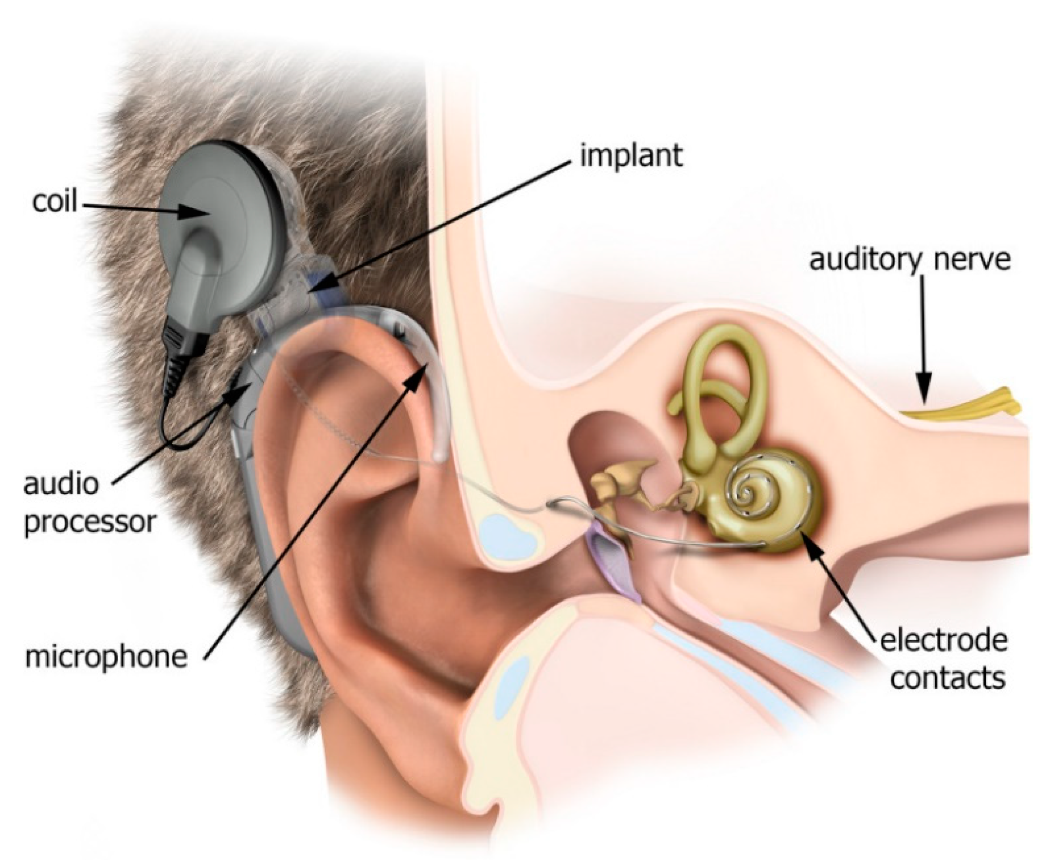
Cochlear implant (CI) surgery is becoming a more viable surgical option for children and adults with substantial sensorineural hearing loss and who have not benefited from hearing aids [1]. The CI system is composed of several parts (Figure 1), such as the external audio processor, microphone, external coil, internal implant, radio frequency (RF) internal coil, and the electrode array that is supposed to be inserted into the scala tympani of the cochlea. The magnetic attraction between the implant magnet and the audio processor coil magnet is used to secure the audio processor coil in place on top of the implant coil. The RF receiver coil also provides the implant with electric power that is emitted from the audio processor coil [2].

The function of the CI microphone is similar to that of the human pinna—it detects and captures the audible sound signals from the area around the patient. The audio processor subsequently uses signal processing algorithms to convert the sound signal into detailed digital signals and transmit them to the internal part (implantable electronics) via the inductive link between the external and internal coil. These digital signals are then converted into electric stimuli/impulses by the electronic system of the internal implant. Thereafter, the electrode array delivers these stimuli to the scala tympani of the cochlea and then to the auditory nerve [3]. The auditory/cochlear nerve should be present in CI candidates as it helps to restore their hearing abilities properly [4]. This nerve acts as a conductor, carrying electrical stimulation generated and decoded by the CI system to the brainstem and then on to the auditory cortex.

CI surgery is typically indicated for pre-lingual and post-lingual deafness. Recently, it has also been approved for patients with single-sided deafness (SSD). Patients who received implants early, before the age of two years, showed better audiological and speech performance [5]. On the other hand, pre-lingually deafened patients of an older age may not show satisfactory outcomes, and they might sometimes be non-users of implants. The explanation behind this is that the brain may utilize the region for auditory sensation at the level of the auditory cortex for other somatosensory inputs after a lengthy period of deafness [6].

The cochlear implant’s (CI) function and the proper placement of the electrode array can be evaluated using different methods, one of which is electrical impedance (EI) measurement [1]. Cochlear implant function is largely based on the device’s ability to reliably send electrical signals to the auditory nerve fibers [7]. This electrical signal can spread easily and widely since the perilymph and endolymph (i.e., intracochlear fluids) are essential electrolytes [2,8]. Therefore, electrical impedance (EI) can be defined as the measure of the reluctance that is expressed by the perilymph to the current flow when voltage is applied [1]. A normal measured impedance range is indicative of a good current flow in the fluid and tissue of the cochlea. Any big variation from the normal range can reflect an abnormal current flow [9].

The value of the impedance is mainly affected by the relationship between the electrode–tissue interface and the surrounding tissues around the electrode. After CI surgery, fibrotic tissue formation is induced by the foreign-body reaction to the electrode [2,10]. The amount of fibrotic tissue surrounding the electrode array has been found to be significantly correlated with EI value. EI reaches its highest value after 4 weeks due to an increase in fibrous tissue formation; then, it stabilizes after 8 weeks. EI declines after the activation of the device due to the disrupted adhesion of the fibrous tissue to the electrode [11].

In clinical settings, testing the EI has the following main uses: for the evaluation of the electrode’s overall function, measurement of the impedance level, detection of problems such as short- and/or open-circuits, guidance for audio processor fitting, and determination of the power consumption level [12]. Clinicians’ familiarity with EI variation trends at different time points after device activation is crucial. This familiarity could also help non-experienced clinicians with any problems they might have with their patients, in case irregular EI values are found. However, there is still a lack of objective tools for predicting the EI at different time points after CI surgery. Therefore, the primary aim of this work is to develop a machine learning model that can utilize specific characteristics of each CI patient to predict the EI at different time points after the surgery and up to twelve months post-activation.

2. Related Work

Machine learning is well-known and has been used in previous studies [13,14]. Many researchers have used machine learning (ML) in projects related to cochlear implantation.

Table 1. Research papers related to cochlear implantation and machine learning.

ID	Ref.	Type	ML Algorithms	Goal	Results
1	[10]	Research	Neural Networks, Linear Regression, and Decision Trees	Predict the electrode impedance after 1 month	Accuracy varies between 66% and 100% based on the channel
2	[15]	Research	Shallow Neural Networks (SNN) and Support Vector Machines (SVM)	Classify the insertion lengths of the electrode array	The SNN accuracy is 86.1% (partial insertion data), while the SVM accuracy is 97.1% (full insertion data)
3	[16]	Research	SVM and random forest	Predict whether healthy people will accept the speech of children with cochlear implants	Random forest algorithm produces the best results
4	[17]	Survey	The study includes 298 articles; The most common ML algorithm is Neural Networks (47.5% of papers)	Determine the usage of ML in CI	Most papers use ML to assist CI in signal processing optimization
5	[18]	Research	Neural Networks and tree-based ensemble algorithms	Predict the postoperative cochlear implant performance	Model accuracy is 95.4%
6	[19]	Research	Random forest	Automate image-guided cochlear implant programming	Recommend specific CI configuration for each patient
7	[20]	Research	Semi-supervised SVM	Predict language outcomes following CI	The model gives a 2-year prediction for developing effective language skills

introduces some of these studies and the most important findings. From these studies, it can be seen that the performance of the ML algorithm differs according to the type and size of the datasets. Many studies use neural networks as a learning model. In this research work, we use different machine learning algorithms, including neural networks. We seek to determine the best algorithm for predicting the electrode impedance in each channel.

3. Material and Methods

3.1. Subjects

This is a retrospective study that was conducted at a tertiary CI center after obtaining ethical approval from the institutional review board. Our inclusion criteria were all pre-lingual children with severe hearing loss who received the same type of CI device (MED-EL, Innsbruck, Austria) at our tertiary center between 2016 and 2018, who had a complete and smooth intraoperative insertion that was assured by post-op X-ray, and who recorded normal EI during the surgery and throughout the follow-up after the device activation. All enrolled patients were full-time CI users, with an average daily use of at least 8.5 h/day and had used their devices for at least 2 years. Patients were excluded if they had cochlear ossifications, inner ear anomalies, or deficient language skills.

3.2. Machine Learning Model

The dataset used in the current study includes 80 patients. For each patient, we compiled the data for age at implantation and the electrode impedance at each electrode contact (from Channel 1 to Channel 12) during the surgery.

Dataset preparation required some formatting standardization processes. These processes were automated using programming scripts written in the Ring programming language [21]. These scripts were generated using the Programming Without Coding Technology (PWCT) software, which is a free/open-source visual programming language for the development of applications and systems [22]. We selected Ring because of its powerful GUI tools in addition to its capabilities, which are comparable to those of Python and Ruby [23].

This study used various algorithms for the regression analyses. We selected some of the popular machine learning algorithms in the literature [24,25,26], such as:

• Neural Networks Regression (NNR);
• Linear Regression (LR);
• Modern decision tree algorithms;

  3.1

  Decision Forest Regression (DFR);

  3.2

  Boosted Decision Tree Regression (BDTR);

• Bayesian Linear Regression (BLR).

Picking one algorithm could lead to limited results. Additionally, we cannot try every possible algorithm to save computational cost and time. So, we decided to pick five different algorithms. Algorithm selection could be based on different factors like the size and the structure of the data, Training time, Accuracy, etc. The survey paper in [18] indicates that the most popular machine learning algorithm used with cochlear implantation datasets in the literature review is the Neural Networks (47.5%). In this survey we notice that the other algorithms do not have huge popularity like the neural networks and the difference between most of them with respect to the usage percentage is not huge. So based on the literature we decided to select (Neural Networks) as our first choice in our list of algorithms that we will use with our dataset. Since we have a regression problem, we decided to select one of the popular regression algorithms in general like linear regression.

After looking at our first two choices (Neural Networks, Linear Regression), We noticed that the function representation of these models is classified as Numerical functions. To have a variety of algorithms, we decided to extend our list with algorithms that use symbolic functions too. and we picked decision trees which is one of the popular algorithms that are useful when working with small dataset as we have. We picked modern decision trees algorithms that uses Ensemble learning like Decision Forest Regression and Boosted Decision Tree Regression (BDTR). Finally, we added the Bayesian Linear Regression algorithm to our list of algorithms as an algorithm that uses (Probabilistic Graphical Models).

We created ML models using Microsoft Azure Machine Learning. We selected this tool to reduce the development time and to facilitate the performance of huge experiments with different parameters that make use of visual tools [27].

Since the dataset is small, and the number of features is limited (from 1 to 13), we used the default settings for each algorithm as provided by Microsoft Azure ML. For neural-network regression the model hyperparameters are (Three layers, Number of hidden nodes = 100, learning rate = 0.005, learning iterations = 100 and the type of normalizer is Min-Max normalizer). For decision forest regression the model hyperparameters are (Number of decision trees = 8, the maximum depth of the decision tree = 32, the number of random splits per node = 128 and the resampling method is bagging). For the boosted decision tree regression, the model hyperparameters are (maximum number of leaves per tree = 20, minimum number of samples per leaf node = 10, the learning rate = 0.2 and the total number of trees constructed = 100). For linear regression the solution method is ordinary least squares and the L2 regularization weight = 0.001.

Since this is a regression problem, we used the Root Mean Squared Error (RMSE) to compare between the different algorithms with the winning algorithm being the one that provides the minimum RMSE. We published the dataset used in this study and the design of the experiments using Microsoft Azure ML in the GitHub website [28].

The following steps were used to build and test the proposed model:

• Preparation of the dataset using the Ring language scripts (generated by PWCT);
• Uploading the dataset to Microsoft Azure Machine Learning;
• Splitting the data (training data and test data);

  3.1

  A total of 70% of the data was used for training (56 patients);

  3.2

  A total of 30% of the data was used for testing (24 patients);

  3.3

  Random seed was used for the splitting process;

• Selecting columns (using features group 1 or 2);
• Selecting the algorithm (from a choice of 5 different algorithms);
• Training the model using the training data and the selected algorithm;
• Evaluating the model (calculating the root mean squared error—RMSE);
• Repeating the experiment and changing the features group and/or the algorithm;
• Comparing the results of different groups of features and algorithms.

3.3. Outcome Measures

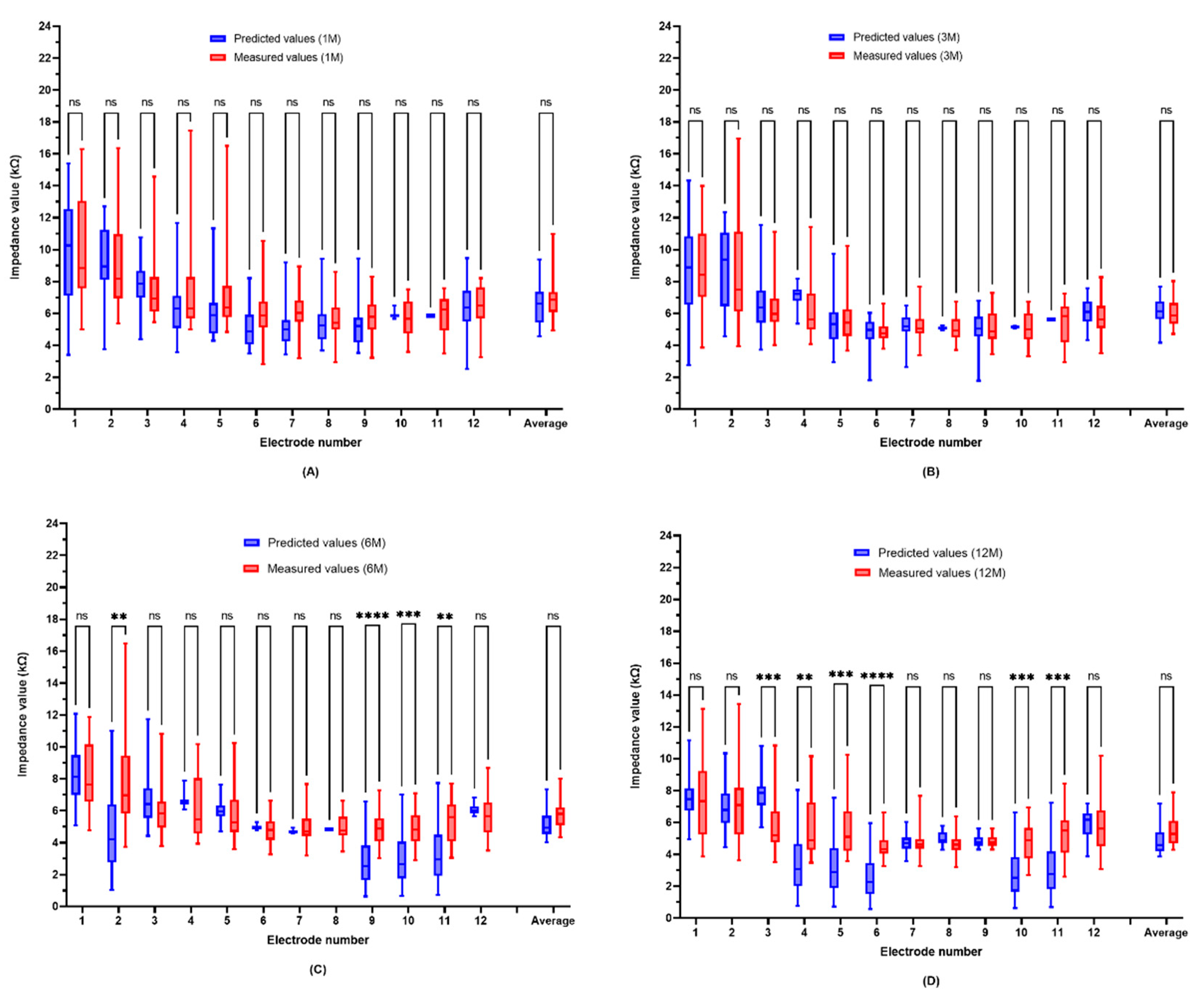
The ML-predicted electrode impedance values were compared to those that were objectively measured and recorded from the included patients. This comparison was carried out for each electrode from the 12 contacts of the tested electrode array at the following time points: one, three, six-, and twelve months post-activation.

3.4. Data Analyses

GraphPad Prism version 9.3.0 was used for all statistical analyses (GraphPad Software, La Jolla, CA, USA). The mean, standard deviation, and range (minimum and maximum values) were used to describe the characteristics of the participants. The normality of the data was first checked before comparing the preoperative and postoperative data. To test the significance of the group data with a normal distribution, a parametric paired t-test was used, and the Wilcoxon non-parametric test was used for the rest of the data. The statistical significance level was set at p = 0.05. The inter-rater reliability, i.e., the degree of agreement among predicted and recorded EI values, was computed using Cohen’s Kappa.

4. Results

The study included a total of 80 patients, which were divided into the study and control groups. The results of the study group represent the predicted EI values, while those of the control group correspond to the measured EI values. The mean age at implantation for both groups was 4.52 years (±2.51 years). Among the included patients, 55% underwent CI on the right side and 45% on the left side.

4.1. Machine Learning Predicted EI Values

Table 2. Dataset features.

Features (Group 1)	Features (Group 2)	Label	Rows
Age at implantation	Age at implantation, EI_Intra_1, EI_Intra_2, EI_Intra_3, EI_Intra_4, EI_Intra_5, EI_Intra_6, EI_Intra_7, EI_Intra_8, EI_Intra_9, EI_Intra_10, EI_Intra_11, EI_Intra_12	One label from (EI_1M_1 to EI_1M_12) or (EI_3M_1 to EI_3M_12) or (EI_6M_1 to EI_6M_12) or (EI_1Y_1 to EI_1Y_12)	80

shows the dataset features and each predicted label. We used the data of both groups to predict the electrode impedance at each contact at one, three, six, and twelve months after the surgery.

Table 3. Minimum and maximum values for each label in the dataset.

	Electrode Impedance (KΩ)
	After 1 Month			After 3 Months			After 6 Months			After 1 Year
Electrode#	Min	Max	Range	Min	Max	Range	Min	Max	Range	Min	Max	Range
1	4.48	16.86	12.38	3.86	15.17	11.31	4.66	14.59	9.93	3.86	14.68	10.82
2	5.37	17.64	12.27	3.94	16.98	13.04	3.21	16.64	13.43	3.02	13.43	10.41
3	4.19	14.57	10.38	4.02	13.88	9.86	3.79	13.2	9.41	3.51	13.2	9.69
4	3.38	17.47	14.09	4.08	11.41	7.33	3.59	10.93	7.34	2.86	11.08	8.22
5	2.71	16.5	13.79	3.66	11.8	8.14	3.59	11.17	7.58	3.32	10.66	7.34
6	2.1	10.55	8.45	3.53	8.72	5.19	3.26	8.15	4.89	3.14	7.25	4.11
7	1.97	8.94	6.97	3.31	7.68	4.37	3.18	7.68	4.5	2.95	7.68	4.73
8	2.34	8.59	6.25	3.38	7.72	4.34	3.41	7.56	4.15	3.2	7.56	4.36
9	2.34	8.3	5.96	3.45	7.33	3.88	2.77	7.29	4.52	2.49	7.29	4.8
10	2.12	8	5.88	2.81	9	6.19	2.51	9.26	6.75	2.7	8.54	5.84
11	2.12	9.62	7.5	2.93	8.08	5.15	3.05	9.76	6.71	2.6	8.71	6.11
12	2.12	9.31	7.19	3.25	9.21	5.96	3.19	9.84	6.65	3.06	11.62	8.56

includes each label in the dataset and the minimum and maximum values. In addition, the table demonstrates the range of values for each label. Some labels have a high range; e.g., for electrode number 4, the EI after one month has a range equal to 14.09 KΩ. On the other hand, some electrodes have a smaller range, such as electrode number 10, which showed an EI of 5.88 KΩ after one month.

After several attempts in testing the machine learning model, we found that

Table 4. The best algorithm and the RMSE.

Electrode#	After 1 Month			After 3 Months			After 6 Months			After 1 Year
	Algorithm	Group	RMSE	Algorithm	Group	RMSE	Algorithm	Group	RMSE	Algorithm	Group	RMSE
1	BLR	2	0.94	BLR	2	0.97	BLR	2	0.85	BLR	2	0.95
2	DFR	2	0.93	BDTR	2	1.03	BLR	1	0.99	BLR	2	0.84
3	LR	2	0.80	BLR	2	0.83	BLR	2	0.72	NNR	2	0.84
4	BLR	2	1.12	NNR	2	0.95	NNR	2	0.97	BLR	1	0.98
5	BLR	2	1.18	BLR	2	0.88	DFR	2	0.87	BLR	1	0.90
6	BLR	2	1.17	BDTR	2	0.78	NNR	2	0.82	BLR	1	0.92
7	BLR	2	1.03	BDTR	2	1.03	NNR	2	0.90	DFR	2	0.93
8	BLR	2	1.05	NNR	2	0.99	NNR	1	0.98	NNR	2	0.87
9	BLR	2	1.09	BDTR	2	0.84	BLR	1	0.94	NNR	2	1.06
10	NNR	2	0.87	NNR	1	0.87	BLR	1	0.83	BLR	1	0.89
11	NNR	1	0.90	NNR	1	1.01	BLR	1	0.95	BLR	1	0.98
12	BDTR	2	0.89	DFR	2	0.92	LR	1	0.77	DFR	1	0.86

contains the best algorithm for predicting the impedance at each electrode in the electrode array. After one and three months, the best algorithm uses Group 2 features, which include the patient’s age and intra-operative EI. After six and twelve months, age at implantation was the best predictor for the EI of half of the electrodes (i.e., six electrodes).

Table 5. The best algorithms for predicting the impedance in the electrode array.

Most Used Algorithm (All-Time)	Count of Labels
Bayesian Linear Regression (BLR)	23
Neural Network Regression (NNR)	13
Decision Forest Regression (DFR)	5
Boosted Decision Tree Regression (BDTR)	5
Linear Regression (LR)	2

demonstrates the best algorithms. It can be seen that Bayesian linear regression is a better algorithm than neural networks. After that, we have the decision forest regression and the boosted decision tree regression at the same level. Finally, we have the linear regression model, which performed well in predicting two labels (out of 48).

In

Table 6. Predicted electrode impedance and the error percentage in different ranges.

Electrode	After 1 Month (%)			After 3 Months (%)			After 6 Months (%)			After 1 Year (%)
	0–1 KΩ	0–2 KΩ	0–3 KΩ	0–1 KΩ	0–2 KΩ	0–3 KΩ	0–1 KΩ	0–2 KΩ	0–3 KΩ	0–1 KΩ	0–2 KΩ	0–3 KΩ
1	20.83	54.16	75	29.16	41	66.66	25	66	78.50	33.33	54.16	79
2	29.16	62.50	66.66	16.66	54.10	66.66	12.50	25	54.16	50	70.83	87.50
3	41.66	62.50	83.33	41.66	79.16	87.50	41.66	62.50	91.66	16.66	41.66	66.66
4	37.50	66.67	83.33	20.83	54.16	95.83	20.83	54.16	100	25	45.83	75
5	54.17	75	83.33	37.50	79.16	95.83	29.20	83.40	95.90	12.50	29.16	58.33
6	41.67	70.83	91.67	62.50	91.66	100	83.40	100	100	20.83	45.83	83.33
7	37.50	66.67	91.67	79.16	87.50	95.84	79.10	95.80	100	75	95.83	100.00
8	41.67	70.83	83.33	66.66	95.83	95.83	66.60	95.70	95.70	66.66	91.66	95.83
9	58.33	79.17	91.67	62.50	91.66	100	20.80	45.80	58.30	62.50	95.83	100
10	58.33	91.67	100	70.83	100	100	25	58.33	70.83	16.66	50	70.83
11	58.33	91.67	100	50	91.66	100	29.20	50	66.70	29.16	50	62.50
12	45.83	54.17	83.33	41.66	79.16	100	54.20	83.40	100	62.50	87.50	87.50

, we list electrodes 1–12 and the different periods, ranging from one to twelve months. Under each period, we assigned three stages of acceptable error ranges: 0–1 KΩ, 0–2 KΩ, and 0–3 KΩ. The number in each cell represents the percentage of the predicted EI that exists in the specified range. For example, 75% of the predicated electrode impedance for electrode 1 at 1 month after surgery exists in the 0–3 KΩ range. Values above 60% are highlighted in the table.

Both

Table 7. The different algorithms and the number of channels where each algorithm provides the best result.

Algorithm	1 M	3 M	6 M	1 Y
LR	1	0	1	0
NN	2	4	4	3
BLR	7	3	6	7
DFR	1	1	1	2
BDTR	1	4	0	0

and

Table 8. The different features groups and the number of channels where each group of features provides the best result.

	1 M	3 M	6 M	12 M
Group (1)	1	2	6	6
Group (2)	11	10	6	6

summarize Table 4. Table 7 provides the winning algorithm for the prediction of the electrode impedance at a specific number of months after the cochlear implant surgery, while Table 8 provides the best group of features used in the prediction.

In Figure 2, we provide a visualization that demonstrates which group of features is more suitable for predicting the electrode impedance of specific channels.

4.2. Machine Learning Predicted EI Values

Hence, we statistically compared the predicted and measured EI values at different time points. One month after the surgery (Figure 3A), the results showed an average EI of 6.55 ± 1.21 KΩ for the measured group, while that predicted by the machine learning model was 6.84 ± 1.23 KΩ. The statistical comparison of both groups revealed a non-statistical difference (p = 0.99). Similar findings exist at the other time points. The average values of the predicted versus measured groups were the following: (i) at three months (Figure 3B) 6.11 ± 0.88 KΩ vs. 6.60 ± 0.83 KΩ; p = 0.99; (ii) at six months (Figure 3C) 5.20 ± 0.87 KΩ vs. 5.77 ± 0.94 KΩ; p = 0.53; (iii) at twelve months (Figure 3D) 4.85 ± 0.90 KΩ vs. 5.51 ± 0.94 KΩ; p = 0.19.

Despite the nonsignificant (ns) differences among the EI of both groups at most electrode contacts at the different tested time points, as illustrated in Figure 1, there are some significant discrepancies between the EI values of specific electrode contacts at two-time points, namely at six months after the surgery (electrodes # 2, 9, 10, and 11) and at twelve months post-op (electrodes # 3, 4, 5, 6, 10, and 11). The stars (**), (***) and (****) in the figure represent the scale of the differences among the EI of both groups.

5. Discussion

A growing body of evidence has demonstrated the utility of machine learning algorithms in predicting and optimizing auditory outcomes following CI. By analyzing large amounts of data, machine learning algorithms can be used to create personalized sound processing strategies for each patient and help in improving the performance of cochlear implants over time. In [23], Alohali et al. evaluated several machine learning algorithms (Table 1) to predict EI one month after surgery. The results showed that the performance of machine learning algorithms was based on the electrode channels, with an accuracy ranging from 66 to 100% [10].

Our experiments indicate that the electrode impedance of CI devices could be predicted at the electrode contacts (from 1 to 12) at different time points using different machine-learning algorithms. Table 6 indicates that the Bayesian linear regression (BLR) provides the best results, followed by the neural networks (NN), which have been used in most research papers related to cochlear implantation [18]. The BLR algorithm provides the best results for seven electrodes when predicting the electrode impedance (EI) after one month of implantation. Furthermore, it provides the best results for three electrodes when predicting the EI after three months. The algorithm provides the best results for six electrodes when predicting the EI after six months, while it provides the best results for seven electrodes when predicting the EI after one year. Therefore, on average, the BLR algorithm provided the best results for half of the electrodes. On the other hand, we noticed that the linear regression algorithm did not provide good results as compared to the other algorithms. When predicting the EI after six months or one year, we noticed that each group of features provided the best results for half of the channels, as demonstrated in Table 7.

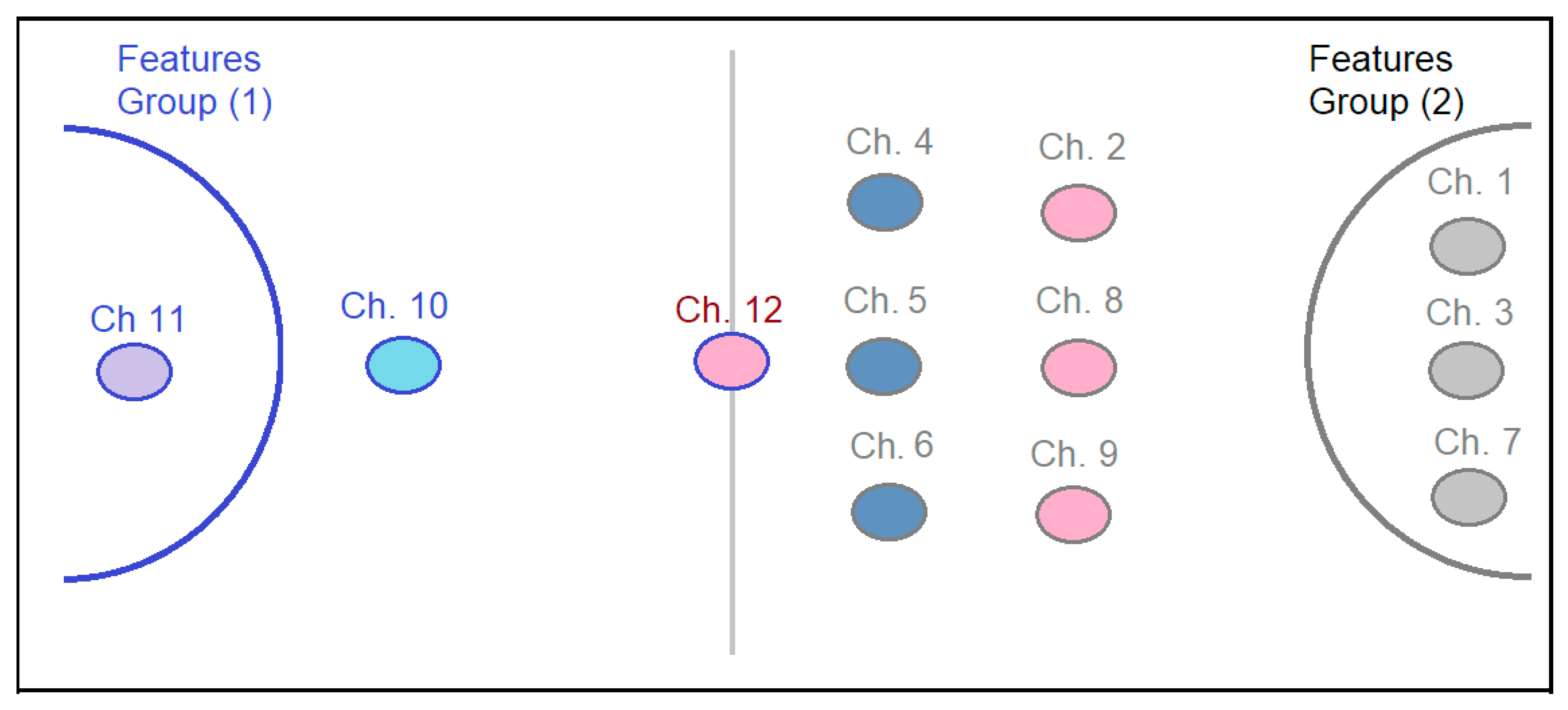
Figure 2 provides a deeper look at the feature groups for predicting the EI of each channel. We noticed that some electrodes provide the best results with a specific group of features, while the other channels shift between the groups based on the period of time. For example, electrode number 11 always provides the best prediction results when using group 1 of the features. However, electrode numbers 1, 3, and 7 always provide the best prediction results when using group 2 of the features. Concerning electrode number 10, after one month, the best prediction results were observed when using feature group 2, while after 3, 6, and 12 months, the best results were achieved when using feature group 1.

When looking at the features that were used to predict EI at different time points, we found that age at implantation and intraoperative EI were the best predictors of EI, with variable accuracies according to the electrode number and time point. Intraoperative EI values can play a significant role in predicting array positioning and helping correct the anatomic and functional placement of the implants [29]. However, the role of intraoperative EI in predicting postoperative function is unclear. Previous reports have shown that abnormal intraoperative EI can significantly predict postoperative electrode function. In [7], there was a trend of persistent abnormalities in the intraoperative EI, which extended to the immediate postoperative period; however, the trend was not statistically significant. Carlson et al. showed that nearly 58% of postoperative electrode abnormalities were observed during the intraoperative period [30]. In the present study, we found that intraoperative EI values can predict EI at different postoperative points.

Electrode numbers 4, 5, and 6 provided the best results for EI prediction using features group 2 after 1, 3, and 6 months, while they provided the best prediction for EI after 12 months using features group 1. On the other hand, electrode numbers 2, 8, and 9 provided the best results for EI prediction using features group 2 after 1, 3, and 12 months, while they provided the best prediction for EI after 6 months using features group 1.

The statistical comparison of the ML-model prediction results and the objectively measured values showed non-significant differences for most electrode contacts at different time points. This could confirm the accuracy and sensitivity of the proposed model. Furthermore, the statistically significant differences could be attributed to the low sample size and the limited number of characteristics that were used to predict the post-op EI levels. However, the application of such a model needs more investigations with a larger sample size before generalizing the findings of the current study. This is due to the small sample size of the current work which could be considered as a study limitation in addition to its retrospective nature. Another limitation is the probability of the existence of some other factors that might influence EI despite the clear inclusion/exclusion criteria of the current study. On the other hand, this model could be used as an initial step for having an objective tool for predicting EI at different time points after CI surgery. Such a tool could assure that the clinicians, even the inexperienced person, will be conversant with EI variation trends at various time points following device activation, and help them to discover any unusual EI values with their patients as earlier as it happens.

6. Conclusions

The results of this study prove that machine learning is an efficient and effective tool in the field of cochlear implantation. Using data processing, feature selection, and machine learning models that employ modern and advanced algorithms, we can predict the electrode impedance of different channels to help professionals make early decisions that would improve the hearing quality of cochlear patients [13,14,15]. In terms of predicting the EI following CI, in this article, we presented a machine learning model that predicted the cochlear impedance in 12 different channels using different algorithms such as linear regression, Bayesian linear regression, random forest regression, boosted decision tree regression, and neural networks. We performed several experiments to evaluate the performance of each model and to determine which model provided the best results at one month, three months, six months, and one year after the surgery.

We developed the model using the Microsoft Azure Machine Learning tool after preparing the dataset using scripts written in the Ring programming language. Through feature selection, we discovered that patient’s age could be used alone to provide the best prediction results for half of the channels at six months or one year after the cochlear implant surgery. Our results also showed that the use of a specific prediction algorithm for each channel provided better results. Furthermore, the accuracy level was between 83% and 100% in half of the channels one year after the surgery, when an error range between 0 and 3 KO was set as an acceptable threshold.