
Near-to-Far Field RCS Calculation Using Correction Optimization Technique

Abstract
:1. Introduction
1.1. Background and Motivation
1.2. Main Contribution
2. Methods
2.1. NF Scattering Model and Amplitude Estimation
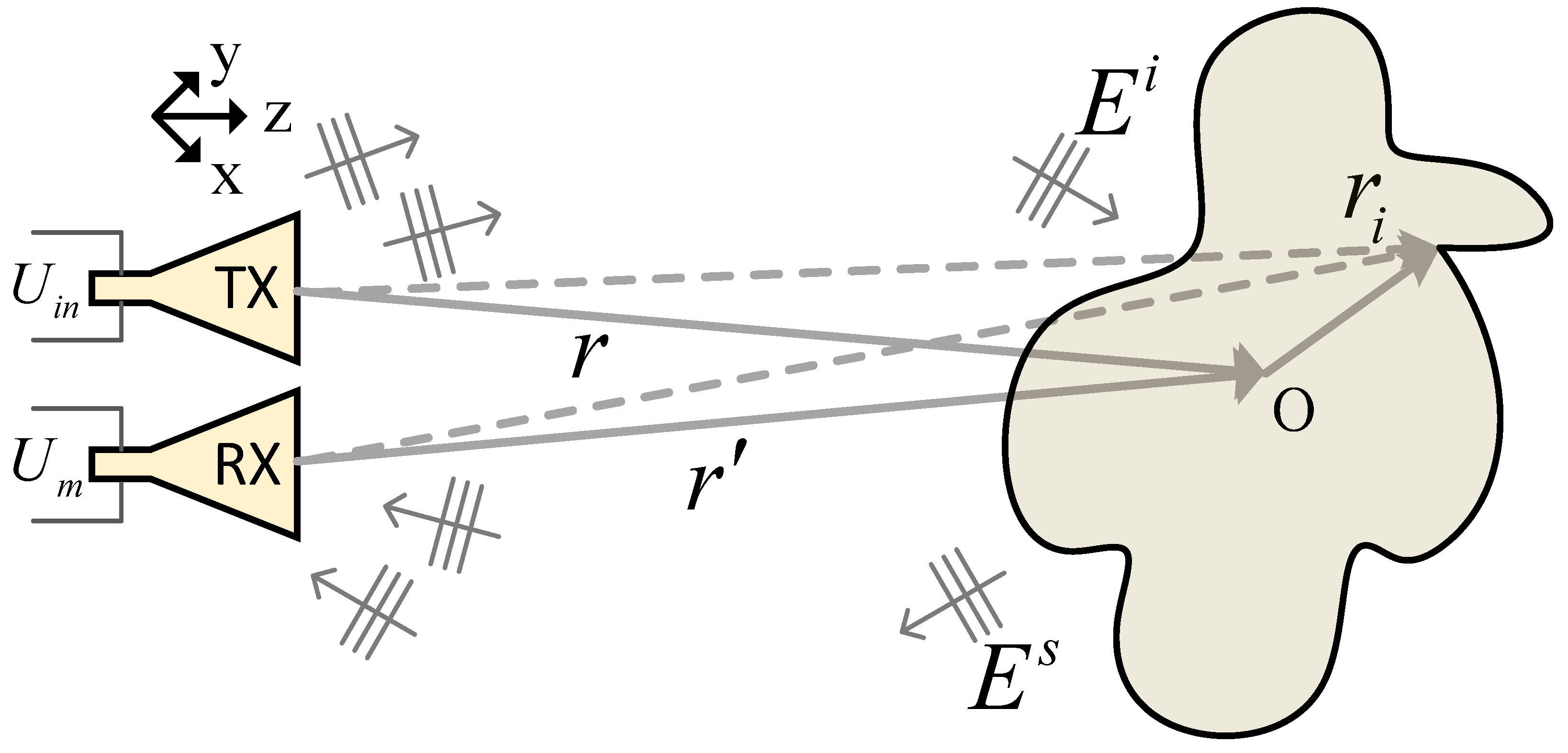
2.1.1. NF Scattering Model
2.1.2. Amplitude Estimation
2.2. Near-to-Far Transformation
2.3. FF RCS Correction
3. Experiments Results and Analysis Discussion
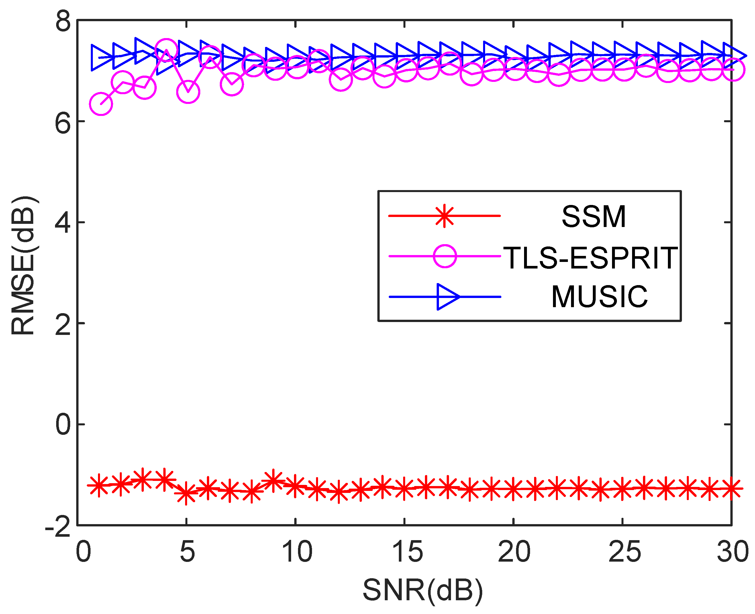
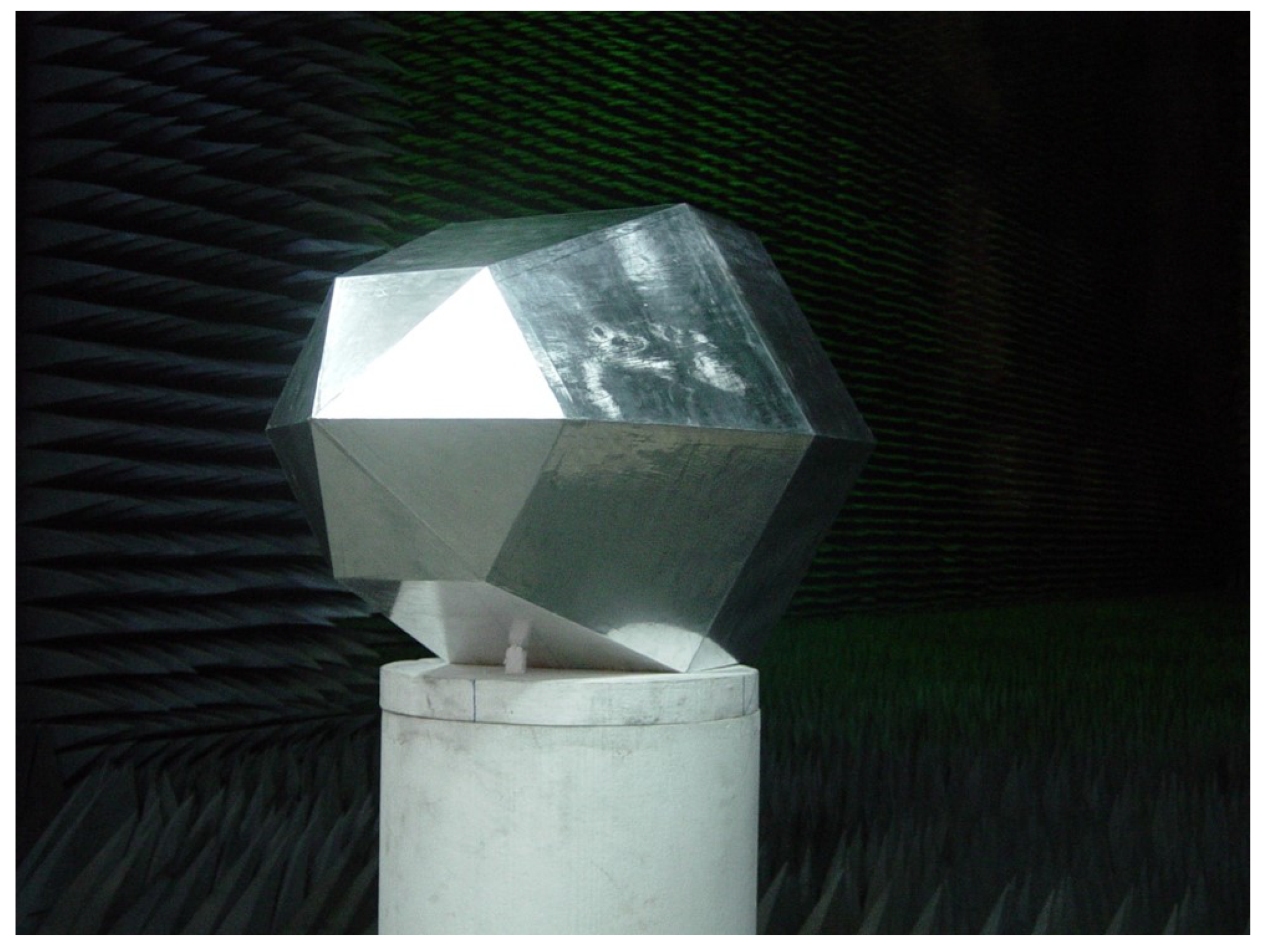
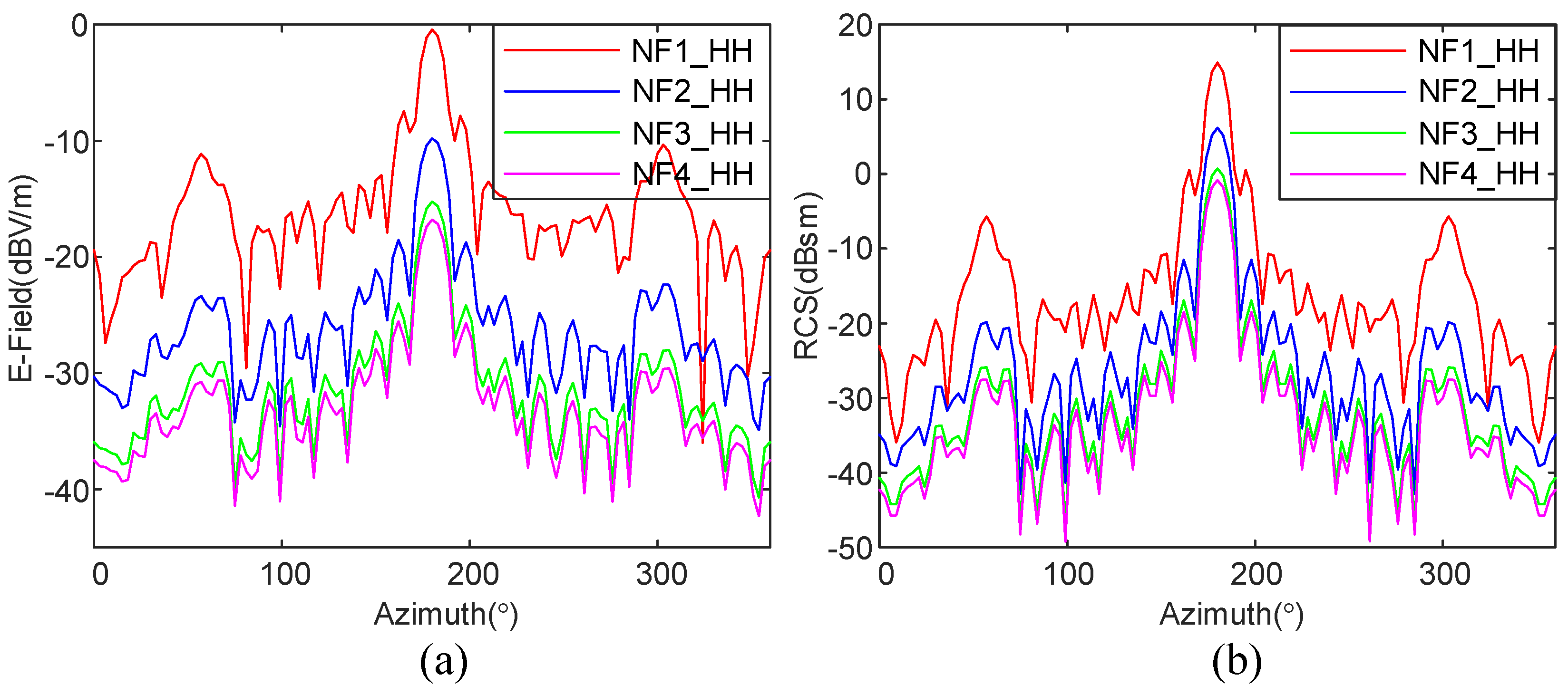
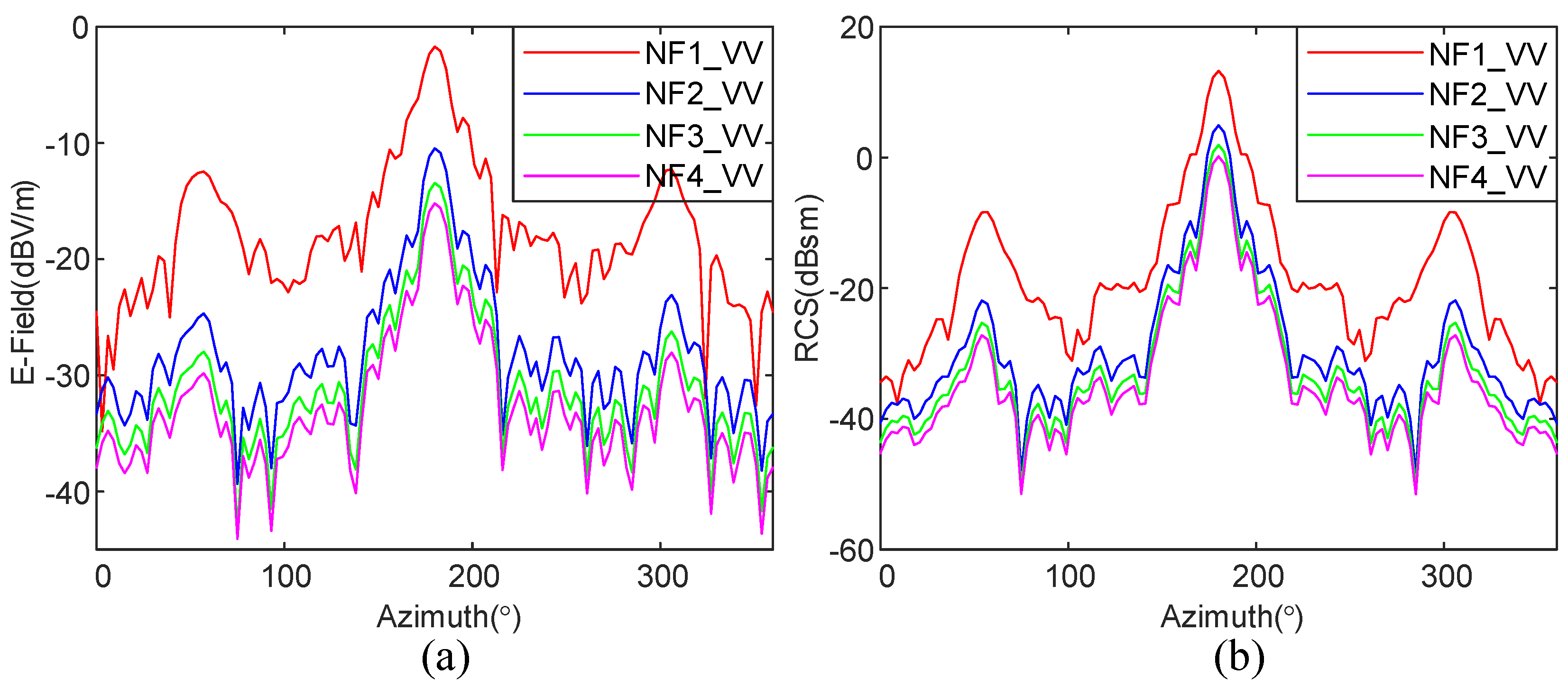
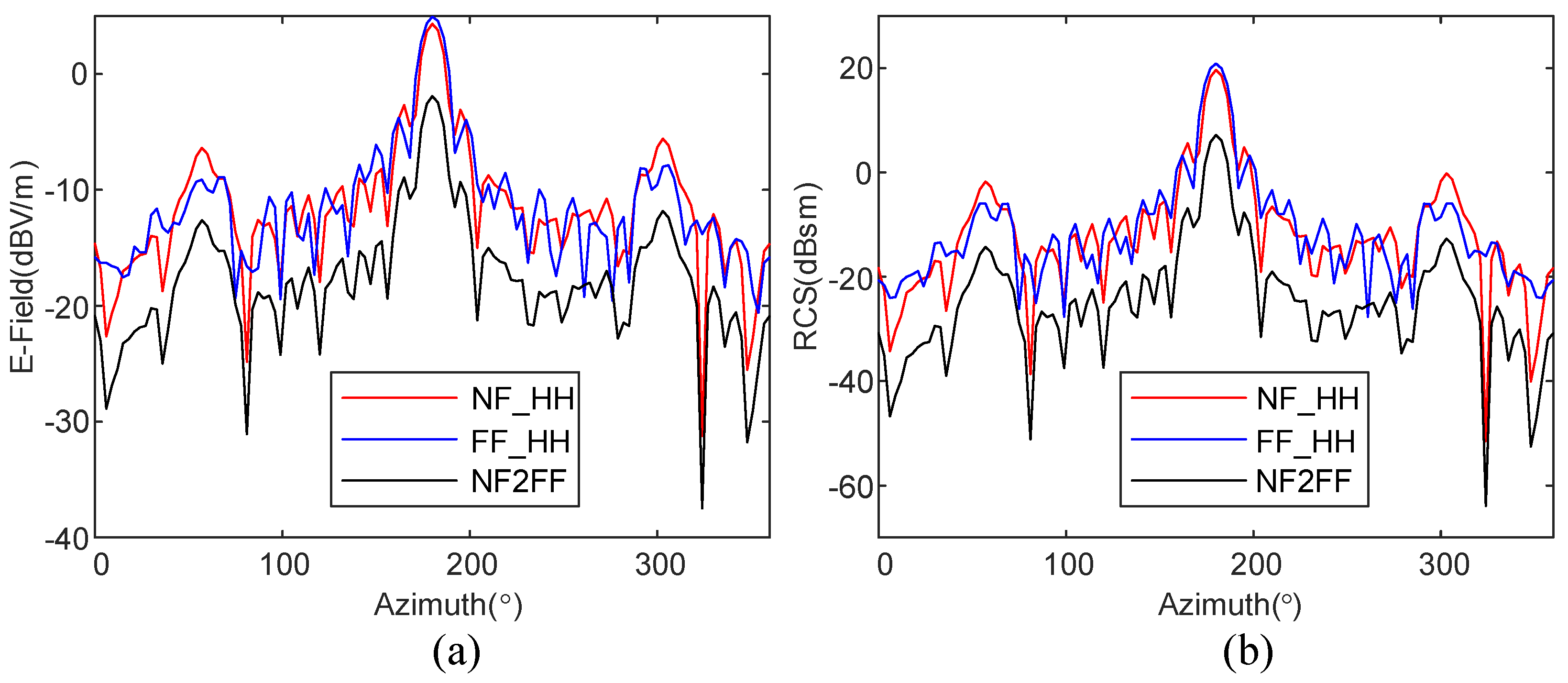
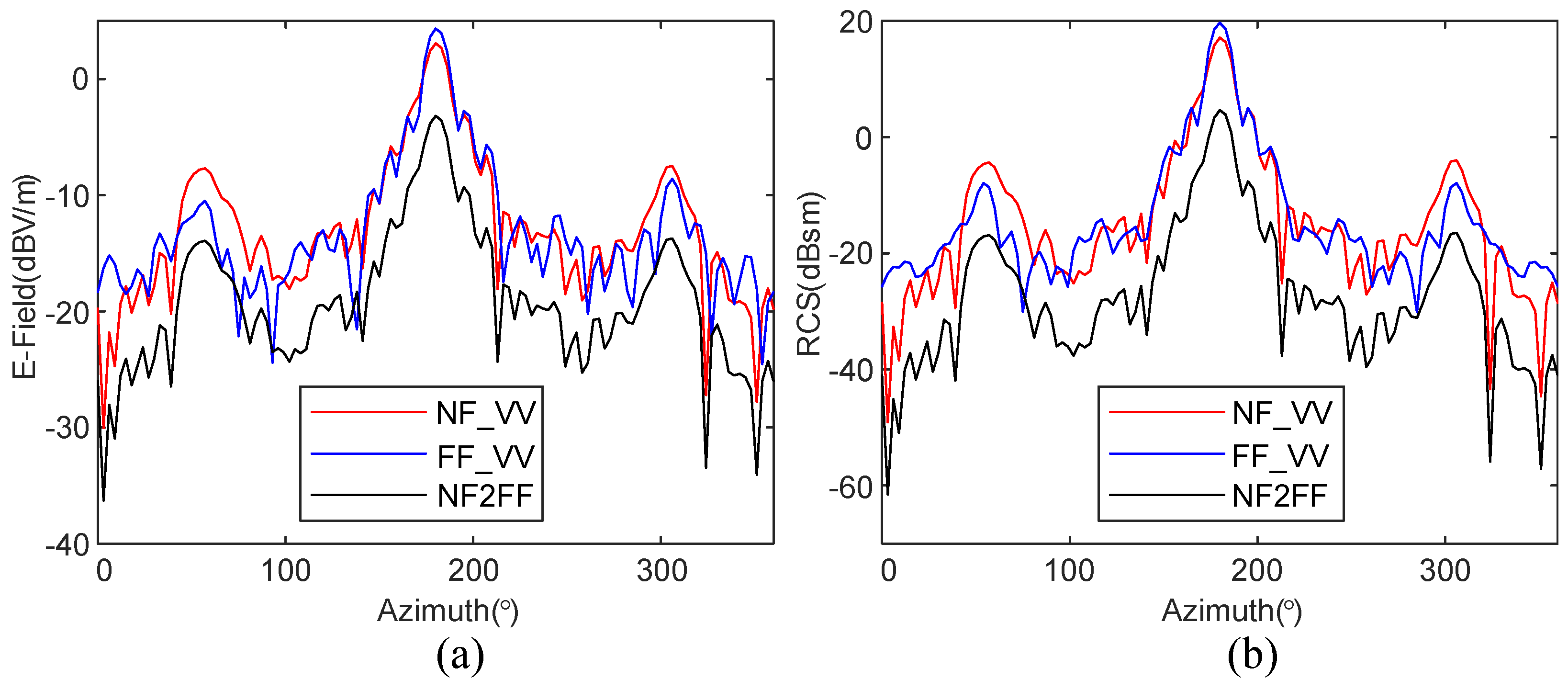
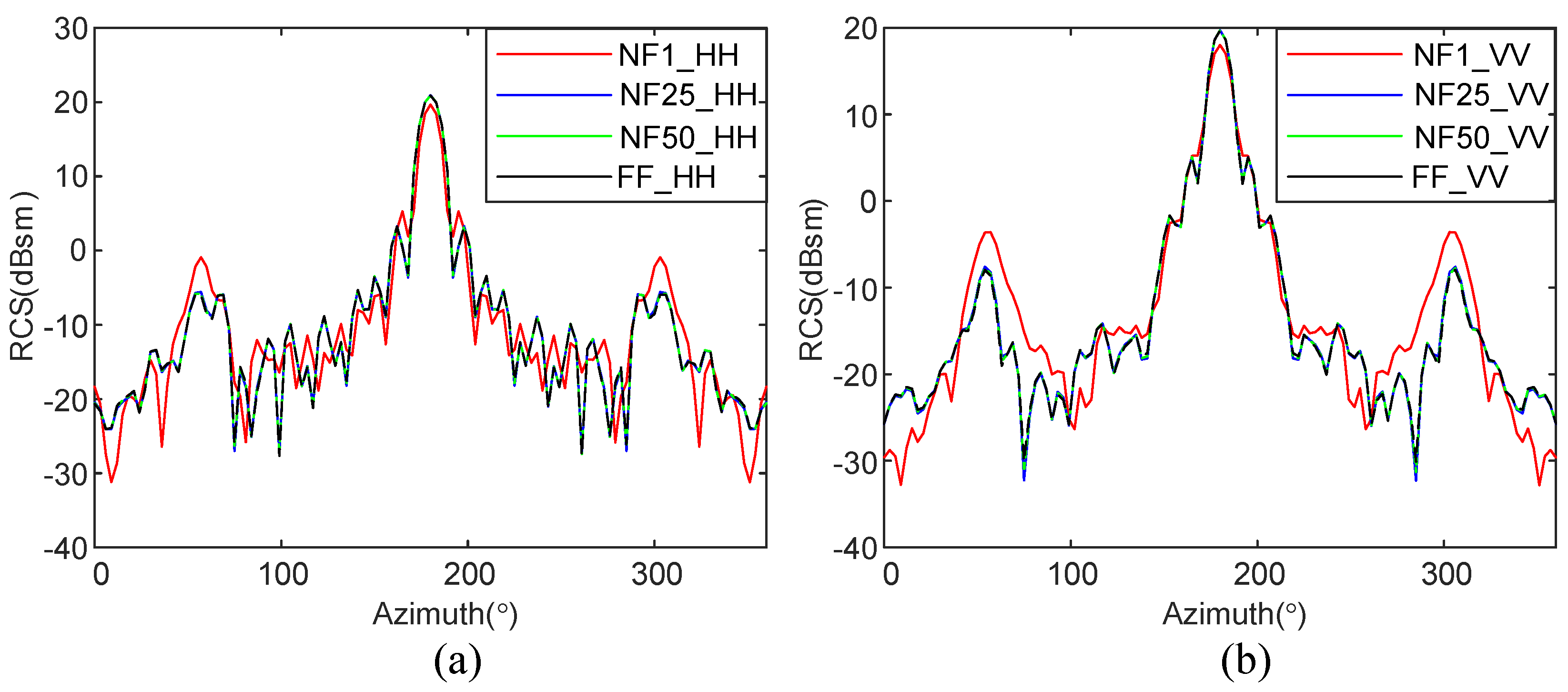
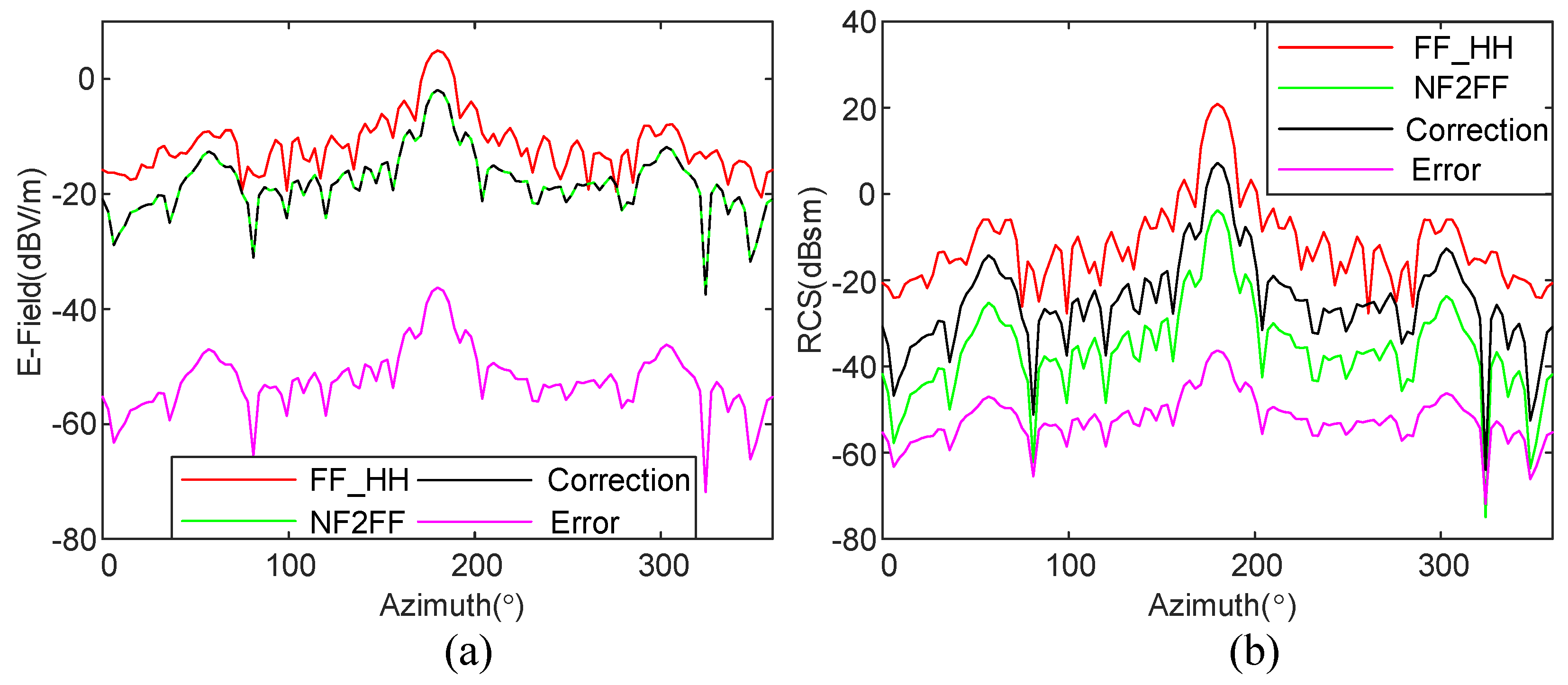
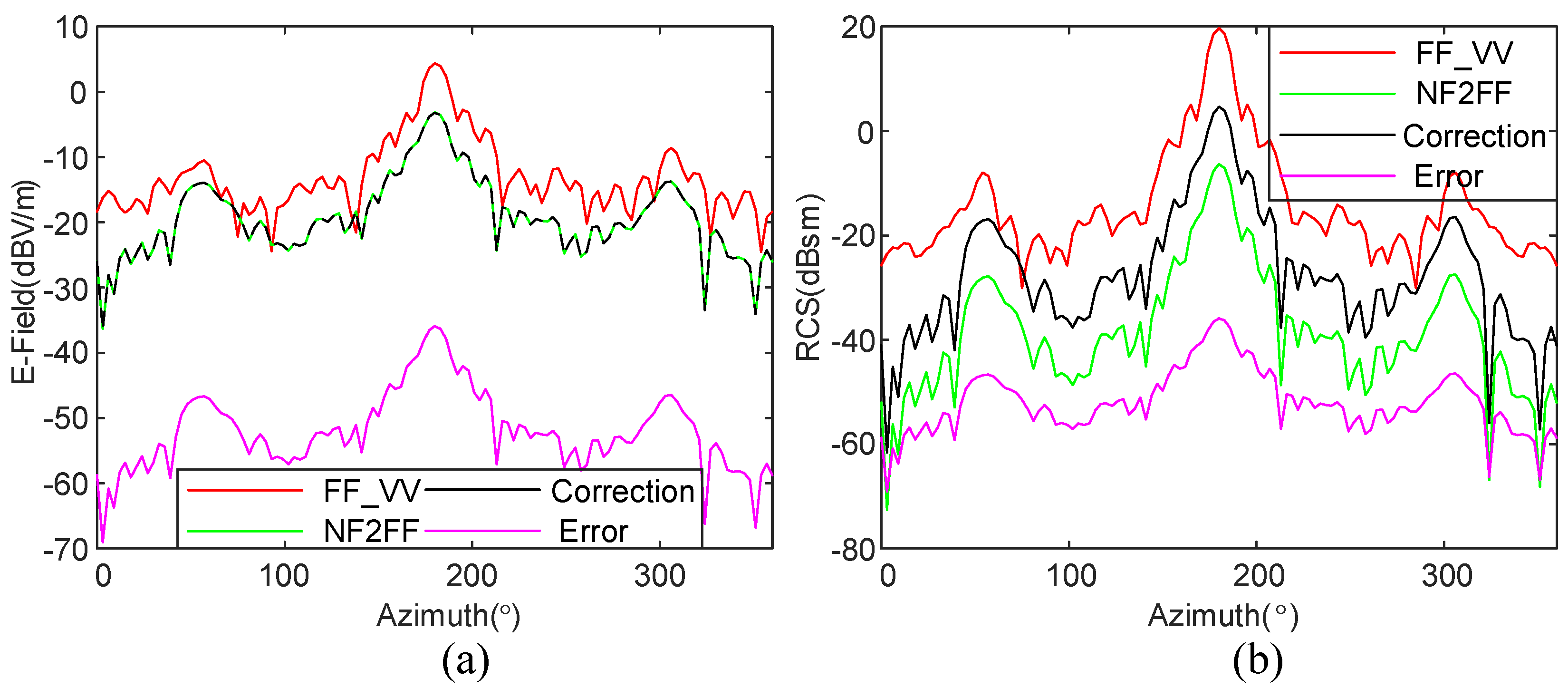
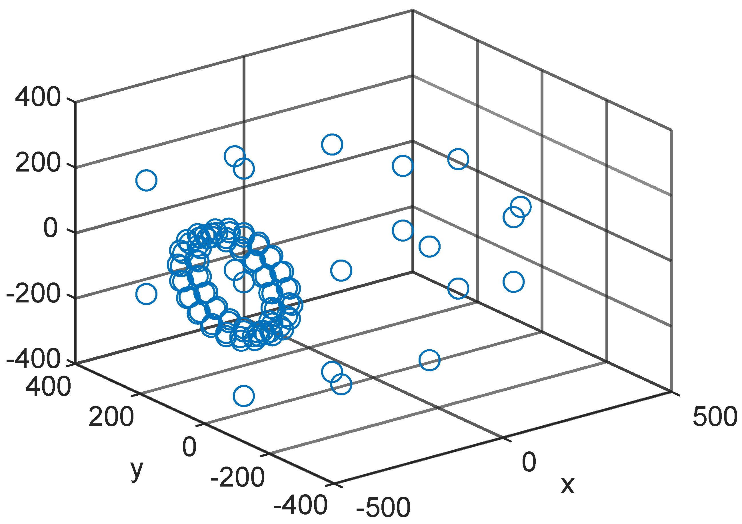
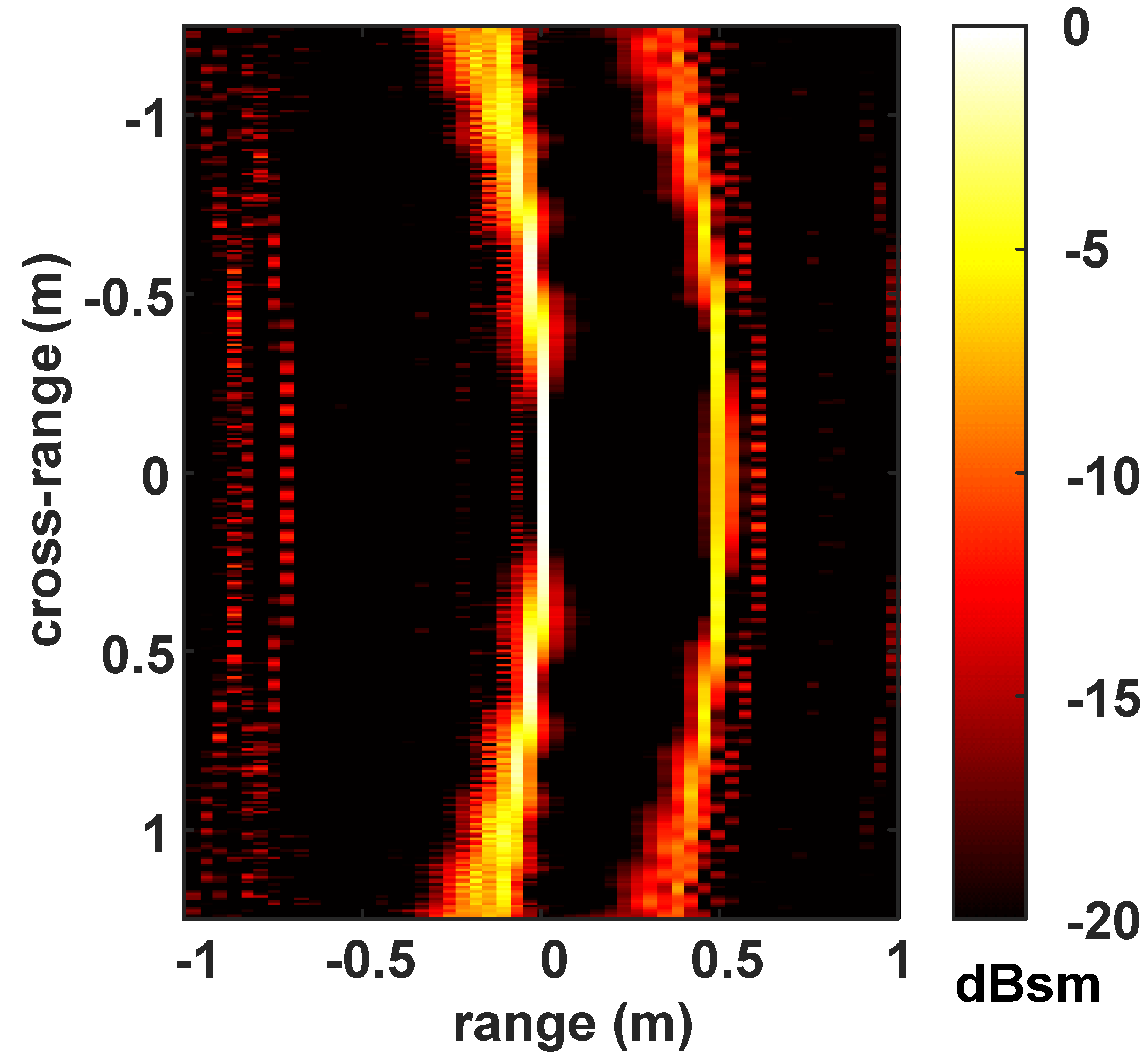
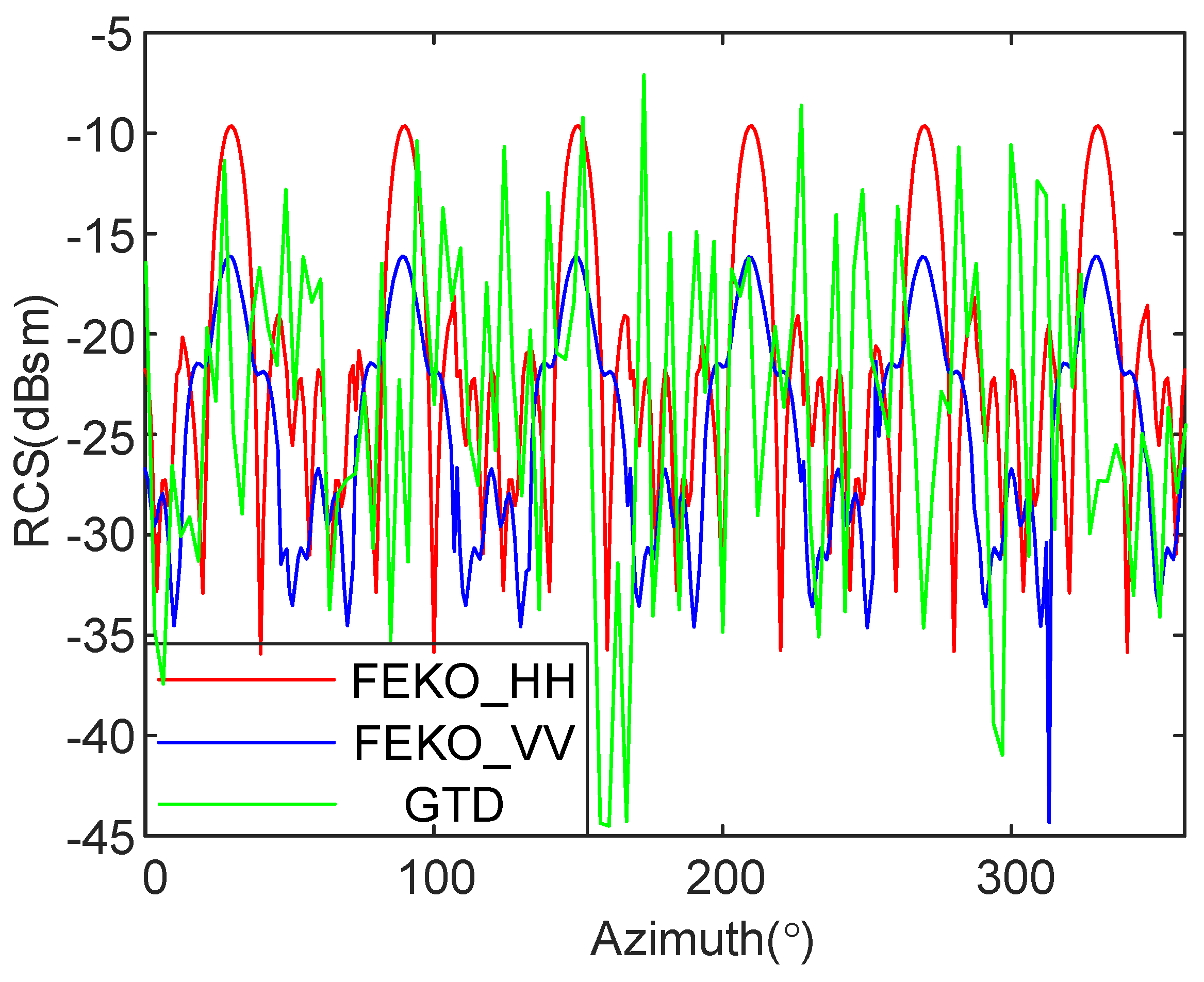
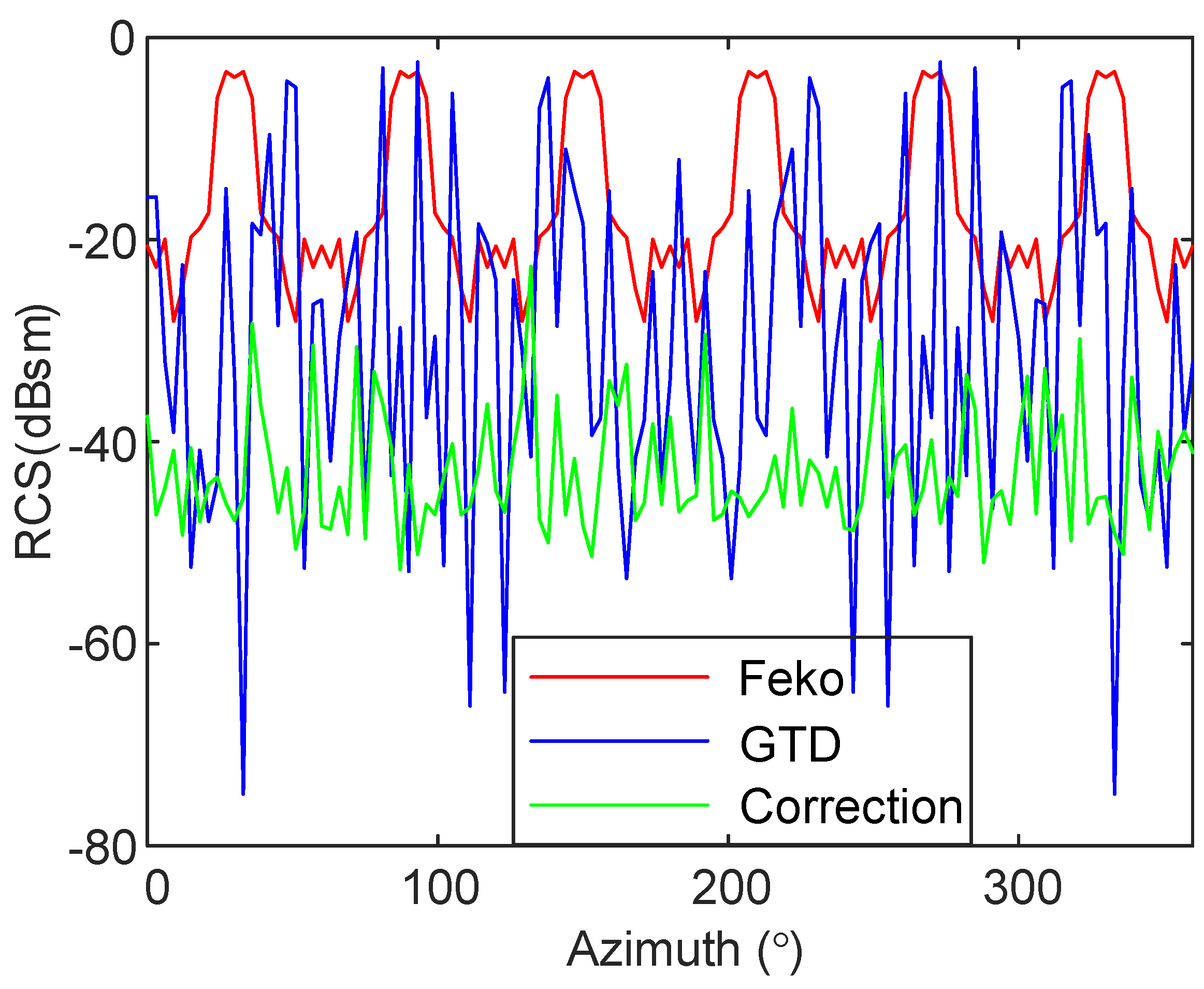
3.1. Experiment 1
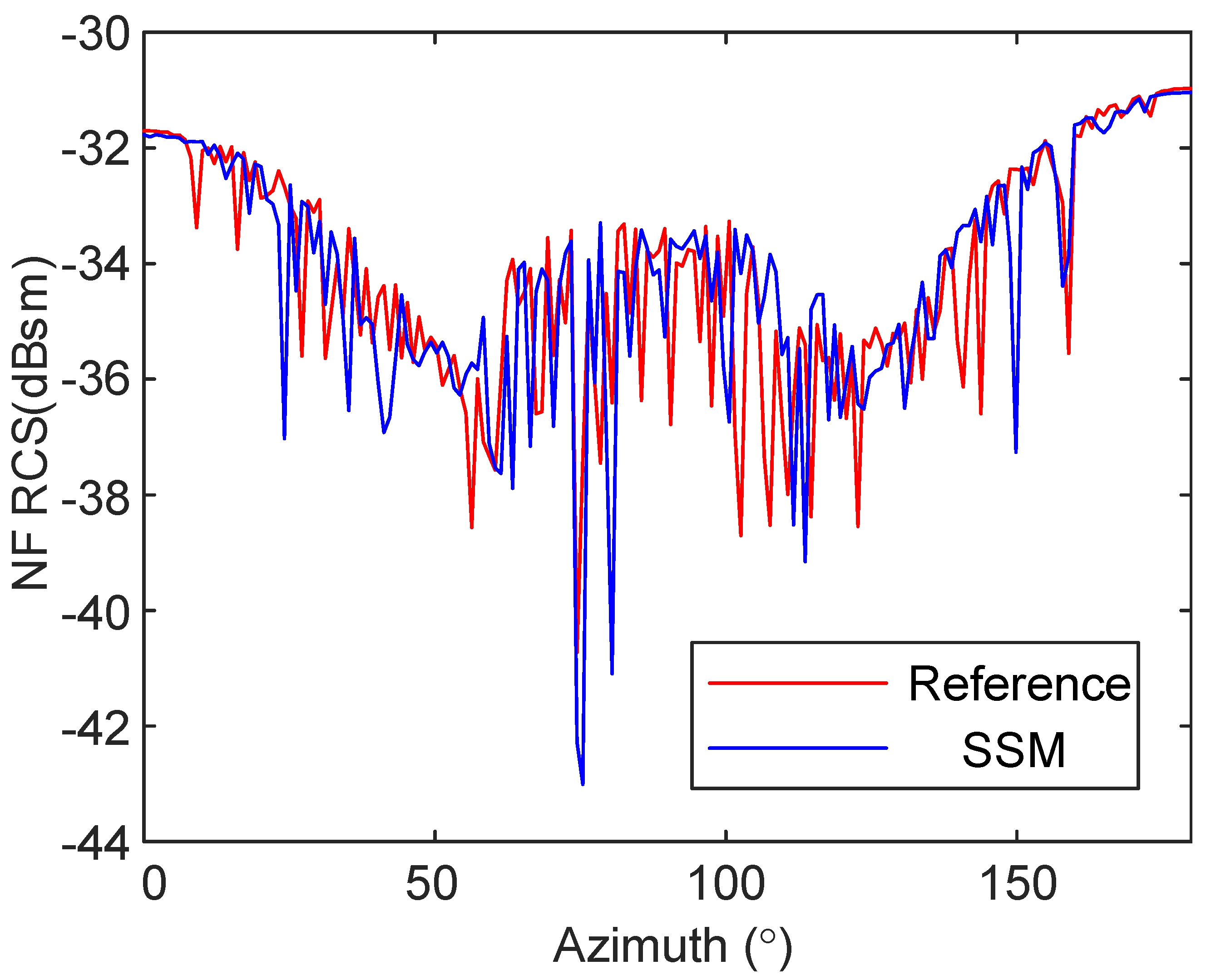
3.2. Experiment 2
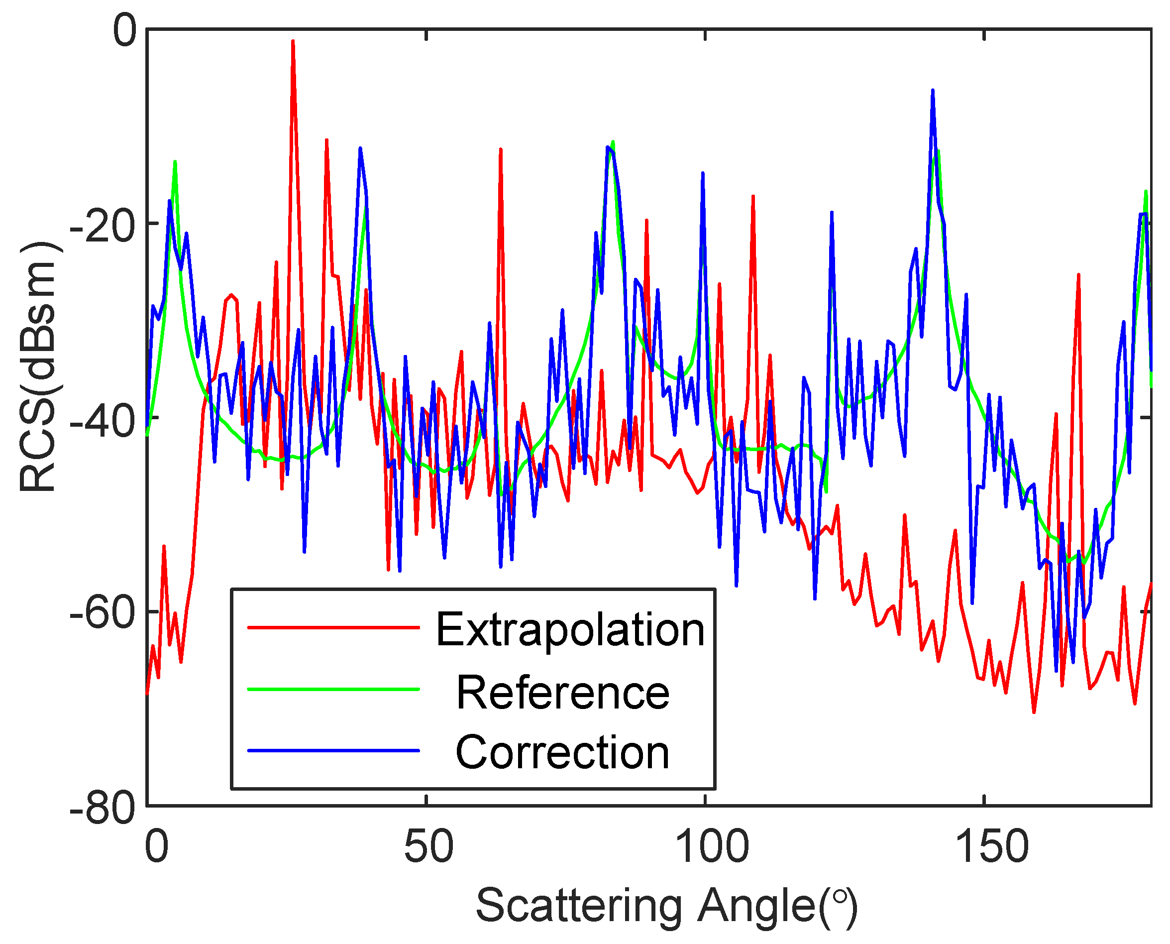
3.3. Experiment 3
4. Conclusions
Author Contributions
Funding
Institutional Review Board Statement
Informed Consent Statement
Data Availability Statement
Conflicts of Interest
References
- Schnattinger, G.; Mauermayer, R.A.; Eibert, T.F. Monostatic radar cross section near-field far-field transformations by multilevel plane-wave decomposition. IEEE Trans. Antennas Propag. 2014, 62, 4259–4268. [Google Scholar] [CrossRef]
- Vaupel, T.; Eibert, T.F. Comparison and application of near-field ISAR imaging techniques for far-field radar cross section determination. IEEE Trans. Antennas Propag. 2006, 54, 144–151. [Google Scholar] [CrossRef]
- Francis, M. IEEE recommended practice for near-field antenna measurements. IEEE Standard 2012, 1720, 5–6. [Google Scholar]
- Qureshi, M.A.; Schmidt, C.H.; Eibert, T.F. Near-field error analysis for arbitrary scanning grids using fast irregular antenna field transformation algorithm. Prog. Electromagn. Res. B 2013, 48, 197–220. [Google Scholar] [CrossRef] [Green Version]
- Schmidt, C.H.; Eibert, T.F. Multilevel plane wave based near-field far-field transformation for electrically large antennas in free-space or above material halfspace. IEEE Trans. Antennas Propag. 2009, 57, 1382–1390. [Google Scholar] [CrossRef]
- Li, J.; Wang, X.; Wang, T. On the validity of Born approximation. Prog. Electromagn. Res. 2010, 107, 219–237. [Google Scholar] [CrossRef] [Green Version]
- Naishadham, K.; Piou, J.E. A robust state space model for the characterization of extended returns in radar target signatures. IEEE Trans. Antennas Propag. 2008, 56, 1742–1751. [Google Scholar] [CrossRef]
- Viberg, M. Subspace-based methods for the identification of linear time-invariant systems. Automatica 1995, 31, 1835–1851. [Google Scholar] [CrossRef]
- Kung, S.Y.; Arun, K.S.; Rao, D.B. State-space and singular-value decomposition-based approximation methods for the harmonic retrieval problem. JOSA 1983, 73, 1799–1811. [Google Scholar] [CrossRef]
- Tripathy, P.; Srivastava, S.; Singh, S. A modified TLS-ESPRIT-based method for low-frequency mode identification in power systems utilizing synchrophasor measurements. IEEE Trans. Power Syst. 2010, 26, 719–727. [Google Scholar] [CrossRef]
- Iordache, M.D.; Bioucas-Dias, J.M.; Plaza, A.; Somers, B. MUSIC-CSR: Hyperspectral unmixing via multiple signal classification and collaborative sparse regression. IEEE Trans. Geosci. Remote Sens. 2013, 52, 4364–4382. [Google Scholar] [CrossRef] [Green Version]
- Potter, L.C.; Chiang, D.M.; Carriere, R.; Gerry, M.J. A GTD-based parametric model for radar scattering. IEEE Trans. Antennas Propag. 1995, 43, 1058–1067. [Google Scholar] [CrossRef]
- Huang, J.; Liu, X.; Zhou, J.; Deng, Y. RCS diagnostic imaging using parameter extraction technique of state space method. Radio Sci. 2023, 58, e2022RS007565. [Google Scholar] [CrossRef]
- Knott, E.F. A progression of high-frequency RCS prediction techniques. Proc. IEEE 1985, 73, 252–264. [Google Scholar] [CrossRef]
- Hu, C.; Li, N.; Chen, W.; Guo, S. A near-field to far-field RCS measurement method for multiple-scattering target. IEEE Trans. Instrum. Meas. 2018, 68, 3733–3739. [Google Scholar] [CrossRef]
- Zhou, J.; Zhao, H.; Shi, Z.; Fu, Q. Global scattering center model extraction of radar targets based on wideband measurements. IEEE Trans. Antennas Propag. 2008, 56, 2051–2060. [Google Scholar] [CrossRef]
- Bunger, R. Time-Domain Evaluation of Full-Wave Scattering Center Models. IEEE Antennas Wirel. Propag. Lett. 2020, 19, 912–915. [Google Scholar] [CrossRef]
- Bao, B.; Xu, Y.; Sheng, J.; Ding, R. Least squares based iterative parameter estimation algorithm for multivariable controlled ARMA system modelling with finite measurement data. Math. Comput. Model. 2011, 53, 1664–1669. [Google Scholar] [CrossRef]
- Ma, H.; Zhang, X.; Liu, Q.; Ding, F.; Jin, X.B.; Alsaedi, A.; Hayat, T. Partially-coupled gradient-based iterative algorithms for multivariable output-error-like systems with autoregressive moving average noises. IET Control. Theory Appl. 2020, 14, 2613–2627. [Google Scholar] [CrossRef]


Disclaimer/Publisher’s Note: The statements, opinions and data contained in all publications are solely those of the individual author(s) and contributor(s) and not of MDPI and/or the editor(s). MDPI and/or the editor(s) disclaim responsibility for any injury to people or property resulting from any ideas, methods, instructions or products referred to in the content. |
© 2023 by the authors. Licensee MDPI, Basel, Switzerland. This article is an open access article distributed under the terms and conditions of the Creative Commons Attribution (CC BY) license (https://creativecommons.org/licenses/by/4.0/).
Share and Cite
Huang, J.; Zhou, J.; Deng, Y. Near-to-Far Field RCS Calculation Using Correction Optimization Technique. Electronics 2023, 12, 2711. https://doi.org/10.3390/electronics12122711
Huang J, Zhou J, Deng Y. Near-to-Far Field RCS Calculation Using Correction Optimization Technique. Electronics. 2023; 12(12):2711. https://doi.org/10.3390/electronics12122711
Chicago/Turabian StyleHuang, Jinhai, Jianjiang Zhou, and Yao Deng. 2023. "Near-to-Far Field RCS Calculation Using Correction Optimization Technique" Electronics 12, no. 12: 2711. https://doi.org/10.3390/electronics12122711