MFLCES: Multi-Level Federated Edge Learning Algorithm Based on Client and Edge Server Selection

Abstract

This research suggests a multi-level federated edge learning algorithm by leveraging the advantages of Edge Computing Paradigm. Model aggregation is partially moved from a cloud center server to edge servers in this framework, and edge servers are connected hierarchically depending on where they are located and how much computational power they have. At the same time, we considered an important issue: the heterogeneity of different client computing resources (such as device processor computing power) and server communication channels (which may be limited by geography or device). For this situation, a client and edge server selection algorithm ($CESA$) based on a greedy algorithm is proposed in this paper. Given resource constraints, $CESA$ aims to select as many clients and edge servers as possible to participate in the model computation in order to improve the accuracy of the model. The simulation results show that, when the number of clients is high, the multi-level federated edge learning algorithm can shorten the model training time and improve efficiency compared to the traditional federated learning algorithm. Meanwhile, the $CESA$ is able to aggregate more clients for training in the same amount of time compared to the baseline algorithm, improving model training accuracy.

1. Introduction

The risk of privacy breaches is increasing, as various Big-Data-driven programs are able to analyze the data left on various smart devices [1], which may result in privacy violations [2]. To tackle this issue, Google proposed the federated learning computing paradigm in 2017 [3]. The FL algorithm differs from traditional machine learning methods [4] in that it does not rely on a shared local dataset. Instead, a shared model is sent by the cloud center server to each client, who trains it locally using their own data and sends the trained model back to the cloud center server [5]. Data privacy security is greatly enhanced because the FL algorithm only requires the transfer of the model to the cloud center server, without any data transfer involved.

Although the issue of data privacy leakage has been addressed, the transmission delay of model data has greatly increased and the training efficiency has been greatly reduced due to the uneven transmission distances of different clients, and the unpredictable and unreliable communication with cloud center servers, which are limited by communication resources [6]. The expansion of the client is a major issue when the training model needs more clients, and sending more model data also somewhat slows down the processing speed of the cloud center server. A new paradigm known as edge computing transfers part of the computing and aggregation tasks from the cloud center server to a group of edge servers that are close to it [7]. This greatly reduces the computational burden on the cloud center server and shortens the communication distance. Meanwhile, as the edge servers can perform preliminary aggregation on the model information sent by clients before sending the aggregated model information to the cloud center server, the cloud center server can receive model information from a larger range of clients for training [8]. Therefore, introducing the benefits of edge computing into $FL$ can greatly compensate for the problems of traditional $FL$ in the scalability of clients. The majority of the current federated edge computing is built with three levels: a cloud center server, numerous edge servers and clients [7]. However, there is still a restriction on the number of visits to clients. Meanwhile, traditional $FL$ algorithms (such as $FedAvg$) randomly select a certain proportion of clients to participate in learning, without considering factors such as client computing power and channel transmission capacity. As a result, once clients are chosen to take part in model training, some of them are unable to upload the model information in a timely manner because of faulty channels or subpar transmission capabilities, which results in a lengthy and ineffective model training process.

Table 1. Summary of the advantages and disadvantages of two-level and three-level federated learning.

	Advantages	Disadvantages
Two-level Federated Learning	Faster training speed with fewer clients	Weak device scalability. Large training delay when there are many clients.
Three-level Federated Learning	Strong device scalability, while reducing training latency and energy consumption.	Usually designed as three tiers and has not been explored for model training over larger geographic areas.

summarizes the advantages and disadvantages of two-level and three-level federated learning.

A multi-level federated edge learning algorithm based on client and edge server selection ($MFLCES$) is suggested in this study as a result of this. These are the unique contributions that this paper makes:

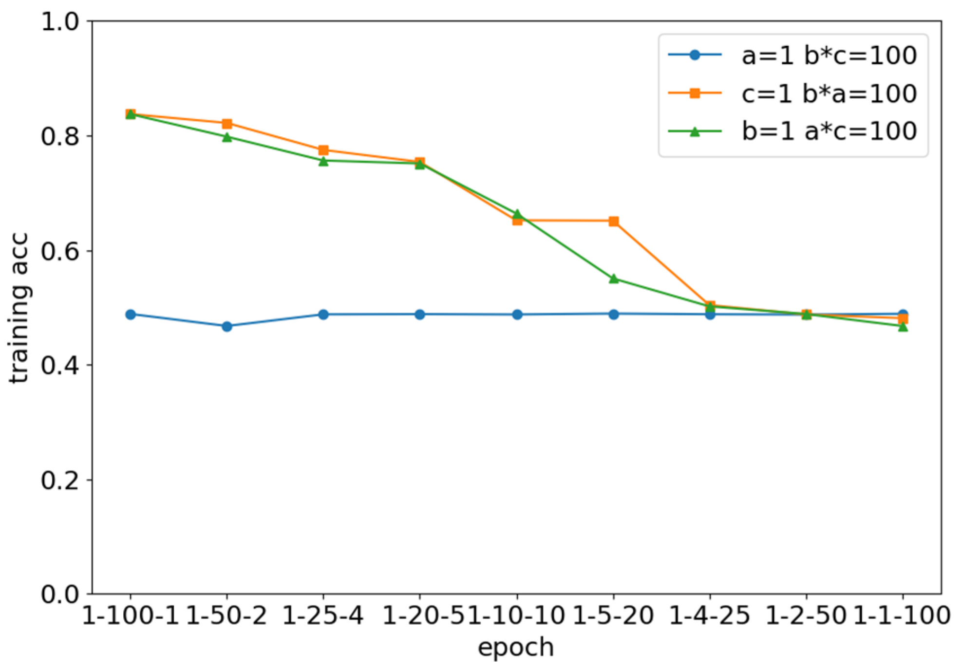
• A multi-level federated edge learning algorithm is proposed based on geographic location and distribution of client computing power. Compared to the current three-level federated learning, the algorithm significantly increases the scalability of the system by fully utilizing the edge server’s capacity to accept additional clients and train a model across a wide geographic area. Simultaneously, the number of communications with the cloud center server is reduced, thus improving the efficiency of model training and reducing the energy loss from communication with the cloud center server.
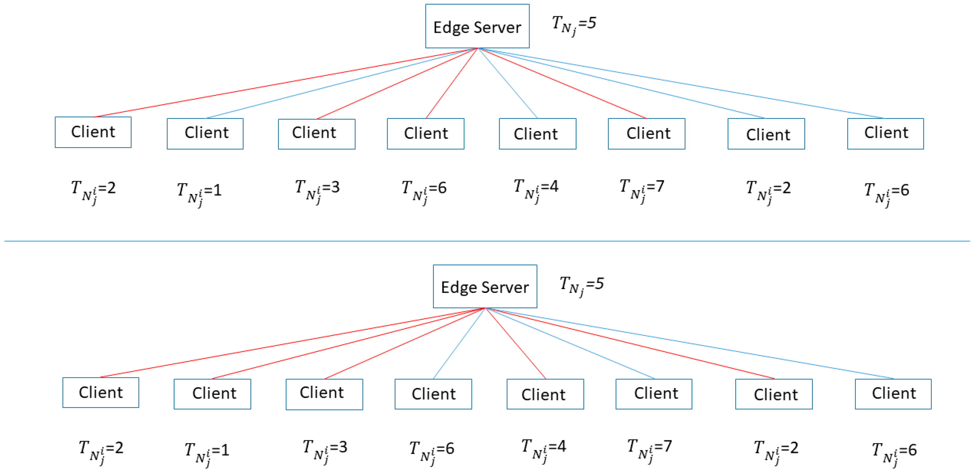
• A client and edge server selection algorithm were designed. Specifically, we have developed a greedy algorithm that sets a deadline for edge server model aggregation and client model updates and uploads. Starting from the cloud center server and moving down each level, the algorithm selects edge servers that can complete model aggregation and upload within the specified time. Similarly, in the second layer, clients who can complete model updates and upload them within the specified time are selected to participate in model training. Compared to the traditional way of randomly selecting a fixed number of devices to participate in training, this algorithm enables the system to aggregate as many edge servers and clients as possible in the same time frame to participate in model training and updates, thereby improving the training accuracy of the model.
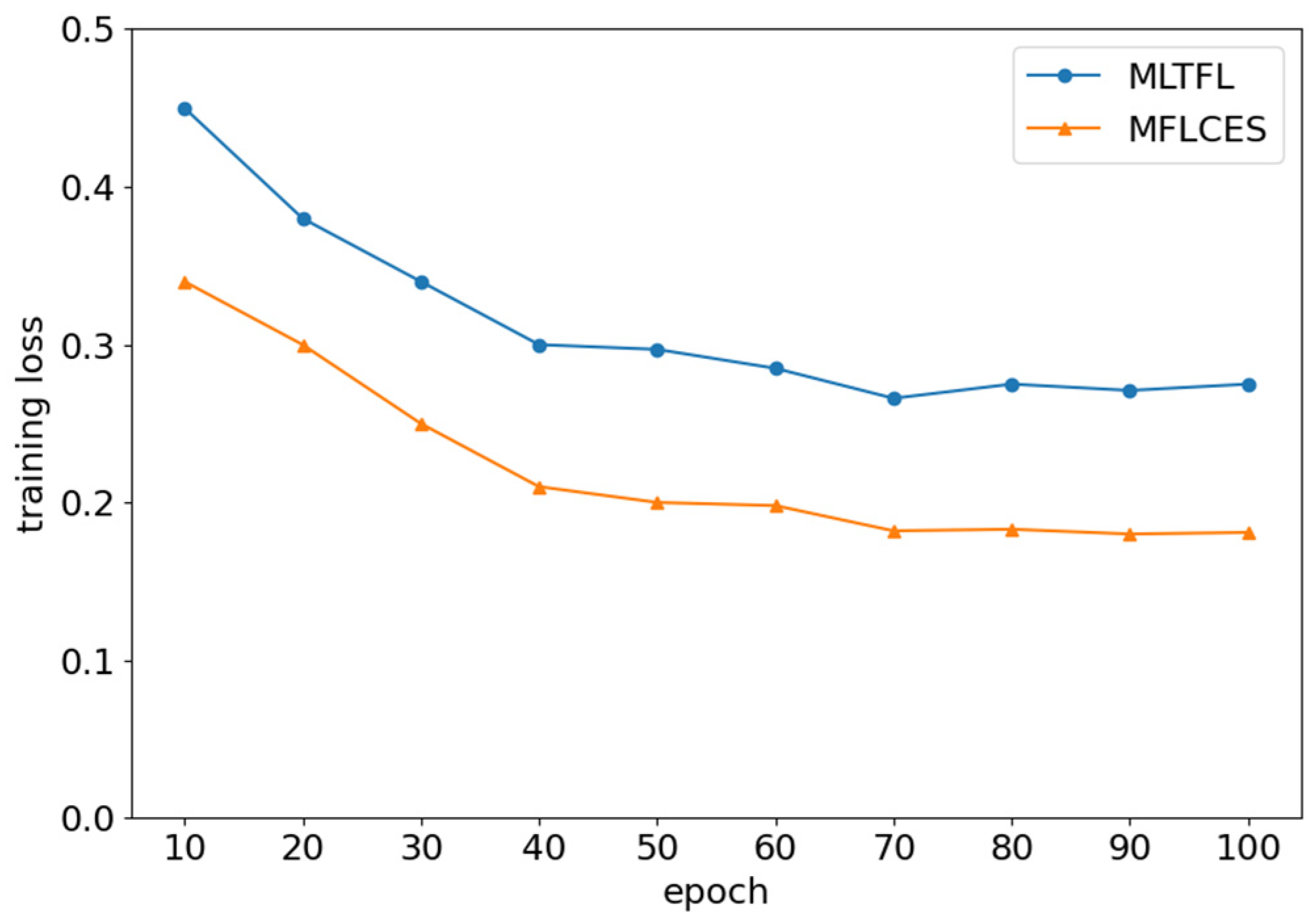
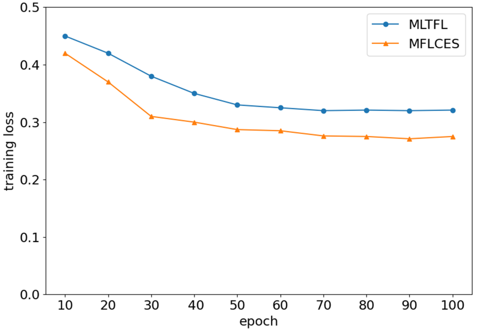
• We conducted simulation experiments on the multi-level federated edge learning algorithm and the client and edge server selection algorithm. The results show that the multi-level federated edge learning algorithm can effectively reduce model training time and improve efficiency as the number of clients increases. Furthermore, compared to the baseline algorithm, the client and edge server selection algorithm can aggregate more clients for training in the same time frame, thereby improving the training accuracy of the model.

The rest of the paper is organized as follows: Section 2 will introduce some related work in $FL$. Section 3 will present the algorithm flow of the multi-level federated edge learning algorithm and the computation of model updates, followed by a detailed introduction of our client and edge server selection algorithm. In Section 4, we conduct simulation experiments and analyze the results. Finally, Section 5 summarizes the entire paper.

2. Related Work

In past few years, $FL$ has produced more scientific research findings. As $FL$’s groundbreaking work, ref. [9] addressed security issues, such as data silos and data leakage, brought on by traditional machine learning that uploaded data to cloud center server and thus proposed the classic $FedAvg$ algorithm. The focus of research shifts as the study goes from how to increase model training accuracy to how to decrease the time and energy loss associated with it. Ref. [10] proposed a $FedCS$ algorithm, which solves a client selection problem with resource constraints, which allows the server to aggregate as many clients as possible for updates, thus improving the accuracy of model training in the same amount of time. Ref. [11] bridged the trade-off problem between $FL$ time and energy consumption for wireless channels by treating $FL$ on wireless networks as an optimization problem $FEDL$, and used the problem structure to decompose and transform the nonconvex $FEDL$ into three convex subproblem, which in turn led to a global optimal solution. Ref. [12] proposed an adaptive enhancement method to improve the efficiency of $FL$. Ref. [13] introduced the concept of learning efficiency as a new performance evaluation criterion. Additionally, a closed expression for allocating communication resources and choosing a batch size is suggested. Two effective radio resource management ($RRM$) solutions for combined bandwidth allocation and client scheduling were developed by [14] after they examined new avenues for energy-efficient radio resource management ($RRM$). To mitigate the degradation caused by $non$-$IID$ data, ref. [15] proposed a hybrid learning mechanism that allows a fraction of clients to upload their data to the server without compromising data security, thus increasing the number of clients involved in $FL$ training. The above work has improved the efficiency of federated learning, but with the increase of intelligent devices, a single server may experience transmission or computation delays due to excessive model transmission and may even experience power overload when there is too much model data.

As technology advances, the Edge Computing Paradigm is put out, and it becomes popular to use it for $FL$ in order to increase the effectiveness of model training. Ref. [7] presented the $HierFedAvg$ algorithm and extended the cloud-client two-level $FL$ model to include edge servers, creating a client–edge–cloud three-level learning model. Not only does the installation of edge servers increase model training accuracy, but also due to fewer contacts with the cloud center server, it also significantly minimizes energy and time loss at the same time. In order to track cumulative privacy losses, ref. [16] offered a privacy-preserving technique for $DP$-based $HFL$ architecture. It also developed a joint computational and communication resource allocation and edge-association problem for clients to accomplish global cost minimization. Ref. [17] integrated a lightweight proof-of-knowledge ($PoK$) consensus mechanism and a blockchain knowledge-sharing architecture into a hierarchical $FL$ system. Comparing the layered framework to conventional blockchain systems, it effectively minimizes computing usage. Ref. [18] considered the impact of client inconsistency and the inconsistency of the information possessed on model training and constructed an $FL$ of inconsistent clients by means of client modeling. Ref. [19] designed a local data evaluation mechanism in $FL$ by considering $non$-$IID$ effects, and developed two optimization strategies for energy service providers. In order to increase the security of model information, ref. [20] suggested a privacy-preserving strategy based on local differential privacy ($LDP$) theory based on hierarchical $FL$, in which clients add noise to shared model parameters before uploading them to the edge and cloud center server. Ref. [21] suggested a hierarchical federated deep reinforcement learning ($HFDRL$) approach that makes use of $FDRL$ techniques to anticipate client demands in the future and choose the best content replacement strategies. Ref. [22] proposed a two-level resource allocation and incentive mechanism, and used evolutionary game theory to model the dynamic clustering selection process. Ref. [23] used gradient sparsification and periodic averaging in heterogeneous cellular networks to improve the communication efficiency of the hierarchical federated learning framework. Ref. [24] separated clustering by introducing a hierarchical clustering step that separates the local updates of clients from the similarity of the globally federated model. Once separated, clusters are trained independently and in parallel on dedicated models. In order to reduce the energy consumption and learning time of resource competition, ref. [25] designed a decoupling algorithm to effectively optimize the client selection and resource allocation problems separately. Ref. [26] established an energy-aware device scheduling problem to allocate communication resources to the optimal subset of edge nodes in order to minimize the global loss function. Ref. [27] proposed an optimal resource allocation method based on federated learning that considers both the delay and energy consumption. Ref. [28] proposed an adaptive asynchronous federated learning ($AAFL$) mechanism that intelligently changes the number of locally updated models for the global model aggregation at different times under different network conditions. Ref. [29] designed a lightweight dual-server secure aggregation protocol that utilizes two servers to achieve secure Byzantine robustness and model aggregation. The above solutions added edge servers to the basic $FL$, but they are mostly based on three-level learning models and have not explored the use of more hierarchical federated learning on a larger geographical scale.

Table 2. Summary of Research Findings.

Two-level Federated Learning	[8,9,10,11,14,15,17]
Three-level Federated Learning	[6,12,13,16,18,19,20,24,25,26,27,28,29,30,31]

provides a summary of the research findings above.

Compared to the studies mentioned above, the multi-level federated edge learning algorithm proposed in this paper explores model training at higher levels and over larger geographic ranges, fully leveraging the advantages of edge computing and greatly increasing the scalability of devices. Meanwhile, the proposed client and edge server selection algorithm can greatly improve the efficiency of model training and enhance the accuracy of model training.

3. System Model

In this section, we detail the $MFLCES$, and we layer all the client according to their computing power as well as their geographical distribution. We therefore abstract the actual client distribution, as shown in Figure 1.

From the outermost to the innermost levels, clients are distributed as 1, 2, …, $Y$. The first level is the edge server level, where a large number of smart devices and various sensors (e.g., smartphones, cameras, etc.) are assembled to receive data around them at all times. They are trained by receiving models from the edge server. The second level, which is next to the edge servers and is connected to a variety of different edge servers, has stronger computation and communication capabilities than the client (e.g., routers, gateways, etc.). The edge server, which is located in the third level and is connected to the edge server in the second level, has higher computational power than the second level (e.g., base station, area server, etc.). Therefore, the final level consists of just one cloud center server. Additionally, we are aware that in the majority of $FL$ cases, clients participate in $FL$ while they are in static settings, such as when a battery is charging [10]. Consequently, we assume that in this design, clients are stable during the learning process and that their geographic position is nearly consistent during this time. However, when model training is carried out, not all clients or edge servers may be able to deliver the trained models to their upper edge servers within the allotted time due to the uncertainty of whether the communication systems of the client can be connected successfully.

3.1. Multi-Level Federated Edge Learning Algorithm Based on Client and Edge Server Selection

In this algorithmic framework, assume a set of mobile clients where $N=\{\mathrm{1,2}\dots \dots N_j\}$, and let $N_j\subseteq N$ denote the $j$-th client of the first level. $E_m^n$ denotes the $n$-th edge server at level $m$ ($2\le m<Y$). Additionally, each client gathers a significant amount of data with tags and creates its own local dataset $D_k=\left(X_k^1,Y_k^1\right)\left(X_k^2,Y_k^2\right)\dots \dots \left(X_k^l,Y_k^l\right)$, where $X_k^l$ represents the $l$-th sample of the $k$-th client, $Y_k^l$ represents the matching tagged output, and $S$ represents the cloud center server at the $Y$-th level.

Table 3. Key notations.

Symbols	Definition	Symbols	Definition
$\mathit{w}$	Global model parameters	${\gamma }_{i:j}$	Bandwidth allocation ratio for client $N_j$
$N=\{\mathrm{1,2}\dots N_j\}$	A set of clients	$a_n$	Achievable transmission rate of client $N_j$
$N_j$	The $j$-th client of the first level	$N_0$	Channel background noise
$E_2^i$	The second-level $i$-th edge server connected to the $j-\mathrm{t}\mathrm{h}$ client in the first level.	$p_n$	Transmitted power
$E_n^m$	The $n$-th edge server of the $m$-th level $(2\le m<Y$)	$h_n$	Channel gain of client $N_j$
$X_k^l,Y_k^l$	The $l$-th sample of the $k$-th client and its corresponding tagged output	$d_j$	Data size of the client model parameter $\mathit{w}$
$\{1\dots Y\}$	System levels	$D_{E_2^i}$	Dataset of all clients under edge server $E_2^i$
$S$	Cloud center server	${\mathsf{\tau }}_e$	Rate of edge server upload model
$D_j$	The dataset owned by the $j$-th client	$t_{edge}$	Latency of edge servers to upload their edge models
$F\left(\mathit{w}\right)$	Global loss function	$D$	Dataset of all clients under the cloud center server
$F_j\left(\mathit{w}\right)$	Local loss function	$T_{finally}$	Final cut-off time
$g$	Updating the index of a step	$A$	The final accuracy to be achieved
$\mathsf{\alpha }$	Gradient descent step	$T_{edge}$	Edge server selection deadline
$\theta$	The required accuracy of the model trained by the client	$T_{\mathrm{c}}$	Client selection cut-off time
$Q\left(\theta \right)$	Number of client local iterations	$t_{agg}$	Time required for edge server aggregation
$\beta$	A constant related to the number of training iterations for a client	$c_n$	$CPU$ frequency assigned to client $N_j$
$q_n$	Number of $CPU$ cycles required for client $N_j$ to process one sample data	$t_j^{cmp}$	Total delay of local iterations of client $N_j$
$B_i$	Total bandwidth provided by $E_2^i$	$t_{j:i}^{com}$	Transmission delay of model parameters uploaded by client $N_j$

summarizes the key notations used in this paper.

The algorithm is divided into seven main steps.

Step 1: Global model initialization

The cloud center server first randomly initializes a global model parameter.

Step 2: Resource aggregation and analysis

The cloud center server cascades the specific requirements of the models that need to be trained down through the edge servers, and all edge servers receive the requests. The request is sent to all of the clients it manages once it reaches the edge server at this level closest to the client. The client receiving the request informs the edge server managing them of their resource information, such as wireless channel status, computing power (e.g., whether they can train the model using a $CPU$ or $GPU$), and the size of the data resource with the type of resource (e.g., if the cloud center server is training a gender recognizer, the client needs to report whether it contains body information pictures and the number of body information pictures it contains). The edge server then gives this information for aggregation and uploads it level by level. At the same time, the edge servers in each level need to pack their own channel status, computing power and other information in turn; upload them to the upper level; and finally summarize this information in the cloud center server.

Step 3: Edge server and client selection algorithm

Each edge server chooses which edge servers it oversees to take part in model updates and aggregation based on the data gathered in Step 2. This process works from the top down, starting with the cloud center server. The selected edge server in this level close to the client likewise estimates the time required by the client it manages for the dataset allocation, model update, and uploading steps based on the information from Step 2, and determines which clients can participate in the next training (the specific $CESA$ is described in detail in the next section).

Step 4: Model downward distribution

The cloud center server transmits the initialized global model from top to bottom, over wireless channels, to selected edge servers and clients at each level.

Step 5: Local Model training and transfer

This phase is divided into two parts: local model update, local model transmission.

• Local model update

For a local client, $N_j$, ${\mathit{x}}_j$ is the input of the client in the $M$-th round, and the matching output is represented by $y_j$. $\mathit{w}$ is the actual vector of the machine learning model with all parameters initialized at the cloud center server in the initial phase. $f\left(x_j,y_j,\mathit{w}\right)$ is the loss function corresponding to this data sample, which represents the error between the prediction made by the model for the $j$-th data sample and the true value. Additionally, the loss function of the dataset $D_j$ for client $N_j$ is $F\left(\mathit{w}\right)$ [30], i.e.,

$$F\left(\mathit{w}\right)=\frac{1}{\left|D_j\right|}{\sum }_{j=1}^{\left|D_j\right|}f\left(x_j,y_j,\mathit{w}\right)=\frac{1}{\left|D_j\right|}{\sum }_{j=1}^{\left|D_j\right|}{f}_M\left(\mathit{w}\right).$$

(1)

To lower the loss function and increase the precision of the model prediction, our training task is repeatedly analyzing the client’s dataset.

The stochastic gradient descent algorithm is the one that is most frequently used in machine learning to update model parameters. The index of the update step is denoted by $g$, and the gradient descent step is denoted by $\mathsf{\alpha }$. The parameters of the model are then adjusted as:

$$\mathit{w}\left(g\right)=\mathit{w}\left(g-1\right)-\alpha \nabla F\left(\mathit{w}\left(g-1\right)\right).$$

(2)

In $FL$, the dataset of all clients is $D$, which is distributed over $N$ clients in the form of ${\left\{D_j\right\}}_{j=1}^N$.The edge server, however, is unable to directly retrieve these datasets scattered across the client. In order to calculate $F\left(\mathit{w}\right)$ in Equation (1), also known as global loss, one must instead use a weighted average across the client local dataset $D_j$ along with a local loss function $F_j\left(\mathit{w}\right)$. Specifically, $F\left(\mathit{w}\right)$ and $F_j\left(\mathit{w}\right)$ are

$$F(\mathit{w})=\frac{\sum _{i=1}^N\left|D_j\right|F_j\left(\mathit{w}\right)}{\left|D\right|},$$

(3)

$$F_j\left(\mathit{w}\right)=\frac{{\sum }_{j\in {\mathit{D}}_{\mathit{j}}}{f}_M\left(\mathit{w}\right)}{\left|D_j\right|}.$$

(4)

In order to achieve the common accuracy $\theta \in \left(\mathrm{0,1}\right)$ required by all local clients, the number of local iterations required by each client is

$$Q\left(\theta \right)=\beta log\left(1/\theta \right),$$

(5)

where $\beta$ depends on the size of the data and the task of machine learning [31].

The number of $CPU$ cycles needed by client $N_j$ to process one sample of data is assumed to be $q_n$. Since each sample ($x_j,y_j$) is the same size, $q_n\left|D_j\right|$ is the total number of $CPU$ cycles required to complete one local loop. We use $c_n$ to represent the $CPU$ frequency associated with client $N_j$, where $c_n\in \left[{c_{}}_n^{min},c_n^{max}\right]$. Consequently, total delay $t_j^{cmp}$ of $Q\left(\theta \right)$ local iterations of the client $N_j$ can be represented as:

$$t_j^{cmp}=Q\left(\theta \right)\frac{q_n\left|D_j\right|}{c_n},$$

(6)

• Local model transmission

Client $N_j$ will send local model parameters $\mathit{w}$ to the associated edge server $E_2^i$ for aggregation after completing $Q\left(\theta \right)$ local iteration. A transmission delay $t_{j:i}^{com}$ will be generated in this process using the orthogonal frequency division multiple access protocol ($OFDMA$). During model transfer, the edge server $E_2^i$ connected to this client provides the total bandwidth $B_i$. Define ${\gamma }_{i:j}$ as the bandwidth allocation ratio for client $N_j$ so that client $N_j$ has an allocated bandwidth of ${\gamma }_{i:j}{B}_i$. Let $a_n$ denote the achievable transmission rate of client $N_j$, which is defined as:

$$a_n={\gamma }_{i:j}{B}_{i}ln\left(1+\frac{h_n{p}_n}{N_0}\right),$$

(7)

where $N_0$ is the background noise, $p_n$ is the transmitted power, and $h_n$ is the channel gain of client $N_j$. Let $d_j$ stand for the data size of the model parameter $\mathit{w}$, and let $t_{j:i}^{com}$ stand for the communication time of client $N_j$ transferring $\mathit{w}$ to the edge server $E_2^i$ [32]. As a result, $t_{j:i}^{com}$ can be written as follows:

$$t_{j:i}^{com}=d_j/a_n,$$

(8)

Step 6: Edge server model aggregation

This phase is divided into two steps: edge model aggregation, and edge model transmission.

• Edge model aggregation

In this step, each edge server $E_2^i$ in the second level receives updated model parameters from the connected client $N_j$ and then performs aggregation:

$${\mathit{w}}_{{\mathit{E}}_2^{\mathit{i}}}=\frac{\sum _{N_j\in E_2^i}\left|D_j\right|\mathit{w}}{\left|D_{E_2^i}\right|},$$

(9)

where $D_{E_2^i}={\cup }_{N_j\in E_2^i}{D}_j$ is the set of data sets of all client under the edge server $E_2^i$. Similarly, the edge server models in the third level are aggregated:

$${\mathit{w}}_{{\mathit{E}}_3^{\mathit{k}}}=\frac{\sum _{E_2^i\in E_3^k}\left|D_{E_2^i}\right|{\mathit{w}}_{{\mathit{E}}_2^{\mathit{i}}}}{\left|D_{E_3^k}\right|},$$

(10)

The remaining levels follow the same pattern.

• Edge model transmission

${\tau }_e$ stand for the rate at which the edge server $E_m^n$ transmits its aggregated model data to the edge servers to which it is linked, and $d_e$ stand for the size of the model parameters of the edge server $E_m^n$. Consequently, we determine an edge server upload latency for its edge model as:

$$t_{edge}=\frac{d_e}{{\tau }_e},$$

(11)

Step 7: Cloud center server model aggregation

The edge server $E_m^n$ conveys the model information to its connected edge server in the upper level through the wireless channel for the next round of model averaging until the model information is conveyed to the last level, i.e., the cloud center server. All of the model data that is received is aggregated by the cloud center server as follows:

$$\mathit{w}=\frac{\sum _{D_{E_{Y-1}^i}\in D}\left|D_{E_{Y-1}^i}\right|{\mathit{w}}_{{\mathit{E}}_{\mathit{Y}-\mathbf{1}}^{\mathit{i}}}}{\left|D\right|}.$$

(12)

We disregard the aggregation time of the cloud center server because it is supported by the model’s most computationally powerful device and has a short aggregation time relative to the edge server and client. The computed model is then sent back from the cloud center server to the client.

Algorithm 1 illustrates the precise algorithm flow. Up until the model achieves a specific required performance or meets the final deadline, all steps aside from initialization will be repeated numerous times on the cloud center server, which aggregates model parameter changes in accordance with Algorithm 1.

Algorithm 1: Multi-level federated edge learning algorithm based on client and edge server selection.

1  Initialization: currLevel =Y, $T_{finally}$, $A$ 2  while T < $T_{finally}$ or currAccuracy < A do 3      while currLevel > 0 do 4        Resource aggregation and analysis; 5        currLevel --; 6      end while 7      while currLevel < Y do 8        Client and Edge server selection; 9        currLevel ++; 10      end while 11      While currLevel > 0 do 12        Model downward distribution; 13        currLevel --; 14      end while 15      While currLevel < Y do 16        Client Scheduled Update and Upload; 17        edge server Aggregation model in a certain time; 18        currLevel ++; 19      end while 20      While currLevel = Y do 21        S aggregate the model; 22      end while 23  end while

3.2. Client and Edge Server Selection Algorithm ($CESA$)

Although we are aware that an increase in clients improves the training accuracy of the model, the longer it takes, the more data about the client model is pooled. Therefore, how to make more clients join the model information training at the same time becomes an increasing goal to be tackled by $FL$. At the same time, due to various practical factors (whether the communication channel is corrupted, signal strength, channel distance of the connected clients, etc.), each client as well as the edge server does not necessarily participate in every model training and aggregation, some clients and edge servers also take a long time uploading the models, which greatly reduces the efficiency of the model training. For this case, we propose a client and edge server selection algorithm ($CESA)$. As stated in Algorithm 2, our goal is to assemble more edge servers and clients to take part in the model training simultaneously. In the second step of the system model, the cloud center server and edge server have been informed about the channel situation, processor capacity and the total amount of data from the client through the resource request and analysis of the respective connected edge servers and client, and the information has been summarized at the cloud center server. We will then choose clients and edge servers using this information. Edge server selection and client selection are the two components of the $CESA$.

(1)

Edge server selection:

The edge servers in level 3 to Y are tasked with receiving model information from the edge servers above and below them, as well as receiving and aggregating the model information from the edge servers below them to which they are connected. Assume that the time used for aggregation of each edge server is $t_{agg}$ and the time used for model transmission of the edge server is $t_{edge}$, as pointed out in Equation (11). Additionally, this element is disregarded because the client time cost for obtaining edge aggregation model parameter $\mathit{w}$ is less than its time cost for uploading edge model parameter $\mathit{w}$ and is nearly constant throughout each cycle. Therefore, the time required for each edge server in training and $t_E$ is:

$$t_E=t_{agg}+t_{edge},$$

(13)

The goal of edge server selection is to obtain more edge servers to join the model training in the same amount of time. Therefore, the time $T_{edge}$ is set for each edge server. For each edge server that can complete model aggregation and uploading within the deadline, the algorithm adds it to the current model aggregation, and for those edge servers that cannot perform aggregation and uploading within the deadline, they are discarded after receiving the uploaded model information and are not added to the model aggregation operation. As in lines 2 to 9 of the algorithm, from level Y down to level 3, each edge server iteratively adds its connected edge servers that can complete the model aggregation and uploads them to the model training task on the deadline.

(2)

Client selection

Similar to the last example, this portion is disregarded because it takes less time for the client to obtain the edge aggregation model parameters $\mathit{w}$ than it does to upload the local model parameters $\mathit{w}$ and is essentially constant throughout each repetition. The client local model training time is shown in Equation (6) as $t_n^{cmp}$. The time required by the client to upload the data model to the edge server they connected to is shown in Equation (8) as $t_{j:i}^{com}$. Similarly, the time used for aggregation at each edge server is assumed to be $t_{agg}$. Therefore, the total amount of time spent during the training period for each client and edge server in levels 1 and 2 is

$$t_j^{cmp}+t_{j:i}^{com}{+t}_{agg},$$

(14)

The goal of client selection is to select as many clients as possible to join the model training task at the same time in order to improve the model training accuracy. As shown in lines 10 to 18 of the algorithm, we designed a greedy algorithm that first sets a deadline $T_{\mathrm{c}}$ and then selects the client with the shortest current response time. Let $T_{N_j^i}$ represent the total amount of time spent during its training period. This time should be added to the total amount of time used by the client who is now selected on the edge server where it is located, $T_{N_j}$. The client is then added to the set of clients $E_2^i$ for the next model training task if the total usage times of the presently used selected clients do not exceed the time restriction $T_{\mathrm{c}}$ imposed by the algorithm. The edge server will keep repeating this process until the cut-off time $T_{\mathrm{c}}$ is reached. Figure 2 provides a graphical representation of the client selection process, and the edge server selection process is similar and will not be further elaborated here.

Algorithm 2: Client and Edge server selection algorithm.

1  Initialization  $t_{agg}$, $T_{edge}$, $T_{\mathrm{c}}$, $S_E=\left\{\right\}$ 2  If  currLevel > 2 and currLevel < Y   then 3    for   $E_2^i$ in   $E_3^k$  do 4          $t_E=t_{agg}+t_{edge}$; 5          $\mathit{i}\mathit{f} t_E<T_{edge}$   then 6                Add  $E_2^i$   to $S_E$; 7        end if 8    end for 9    end if 10   If  currLevel = 2   then 11     for  $N_j$ in $N$ do 12        $T_{N_j^i}\leftarrow arg\underset{j\in K^{\prime }}{max}\frac{1}{t_j^{cmp}+t_{j:i}^{com}{+t}_{agg}}$; 13        $T_{N_j}\leftarrow T_{N_j^i}$; 14        if $T_{N_j}<T_{\mathrm{c}}$ then 15             Add $N_j^i$ to $E_2^i$; 16       end if 17   end for 18 end if

4. Experiment

4.1. Simulation Settings

A simulation of a cellular network in a city was conducted, which utilized the $MNIST$ dataset consisting of 10 classes of handwritten digit images to train the model. The neural network model used was $LeNet$, which included three convolutional levels, two pooling levels, and one fully connected level. Each client utilized mini-batch stochastic gradient descent ($mini$-$batchSGD$) with a batch size of 20, an initial learning rate of 0.01, and a decay rate of 0.992 [7] for each learning rate. The three deadline settings were $T_{edge}$ set to 3 min, $T_{\mathrm{c}}$ set to 3 min, and $T_{finally}$ set to 360 min [11].

The experiments were conducted on a Windows 11 operating system with an AMD Ryzen 7 5800H 3.2 GHz CPU (produced by Advanced Micro Devices (AMD), a company based in the Santa Clara, CA, USA), GeForce RTX 3050 Ti GPU (produced by NVIDIA, a company based in the Santa Clara, CA, USA), and 16 GB RAM. We used Python 3.9 and PyTorch on PyCharm 2022 version. to conduct our experiments. The following models of wireless communication and local computing will be provided. Each edge server has a maximum bandwidth range of [1, 10] MHz, and edge servers with different channel transmission capabilities have different maximum bandwidths. The client has a transmission power of 200 $\mathrm{m}\mathrm{W}$ and a $\mathrm{C}\mathrm{P}\mathrm{U}$ frequency in the range [1, 10] $\mathrm{G}\mathrm{H}\mathrm{z}$ with a power of 600 $\mathrm{m}\mathrm{W}$. The processing density of the learning task is [10, 100] $\mathrm{c}\mathrm{y}\mathrm{c}\mathrm{l}\mathrm{e}/\mathrm{b}\mathrm{i}\mathrm{t}$. Similarly, clients with different computing power have different CPU frequencies and processing densities for learning tasks. The background noise is ${10}^{-8} \mathrm{W}$ [16], the client training size is [5, 10] $\mathrm{M}\mathrm{B}$, the updated model size is 25,000 $\mathrm{n}\mathrm{a}\mathrm{t}\mathrm{s}$, and the capacitance factor is ${2\times 10}^{-28}$.

(1) The first step is to investigate the impact of different numbers of client on the training of the two-level $FL$ algorithm and the multi-level federated edge learning algorithm proposed in this paper. The number of clients and servers corresponding to each training for the two architectures are deployed as shown in

Table 4. Number of servers used for training with different numbers of client in the multi-level federated edge learning algorithm.

The number of clients	400	600	800	1000
The number of edge servers in the second level	40	60	80	100
The number of edge servers in the third level	20	30	40	50
The number of cloud center servers	1	1	1	1

and

Table 5. Number of servers used for training with different numbers of client in the two-level federated learning algorithm.

The number of clients	400	600	800	1000
The number of cloud center servers	1	1	1	1

.

(2) Secondly, we will investigate the training accuracy of the edge and client selection algorithms. For the multi-level federated edge learning algorithm, we designed a four-level architecture with 400 clients in the first level, 40 edge servers in the second level, 20 edge servers in the third level, and one cloud center server in the fourth level. In consideration of the fact that edge servers, such as routers and gateways, typically have strong computing power and a stable energy supply in practical applications, we do not take into account the edge model aggregation time and energy cost during model training and optimization. Therefore, the time used by each edge server to aggregate the model, $t_{agg}$, is set to 0 [10]. Moreover, assuming that all clients have consistent channel conditions, the model transmission time is also consistent. Thus, the decisive factor for the client’s model training and transmission time is the client’s computing power, with stronger computing power resulting in shorter computing time.

(3) Finally, we will investigate the impact of different levels of aggregation frequency on training accuracy for the multi-level federated edge learning algorithm based on client and edge server selection. The experimental settings are the same as in the second step.

4.2. Experimental Results and Analysis

(1) To train the two-level $FL$ algorithm and multi-level federated edge learning algorithm to a training accuracy of 0.7, for the multi-level federated edge learning algorithm, each edge server in the second level selects its connected clients to participate in model training at a ratio of ${\mathrm{C}}_1=0.1$. The third level and cloud center server select the connected edge servers to participate in model training at a ratio of ${\mathrm{C}}_2={\mathrm{C}}_3=0.1$. Similarly, the two-level $FL$ architecture selects its connected clients to participate in model training at a ratio of ${\mathrm{C}}_1=0.1$. For different numbers of client, the training time for each training is as follows:

In Figure 3, the x-axis represents the number of clients, and the y-axis represents the time required to reach the training accuracy. From the experimental results, it can be seen that when the number of clients is small, the traditional two-level $FL$ requires less training time. However, as the number of clients gradually increases, the time required for the multi-level federated edge learning algorithm becomes shorter compared to the traditional two-level $FL$. This is because the introduction of edge servers shortens the model transmission distance of local client, and the required transmission time is correspondingly reduced. At the same time, for the same number of clients, compared to traditional two-level $FL$, the multi-level federated edge learning algorithm has a reduced workload due to the decreased amount of the model processed by the cloud center server. Therefore, when the workload is the same, the multi-level federated edge learning algorithm can aggregate the model information from more clients over a larger geographical range, greatly increasing the scalability of the system.

(2) The traditional $FedAvg$ algorithm assumes the existence of a cloud center server and client $N$, selecting clients to participate in model training with a proportional ratio $C$ in each training iteration. We slightly modify the traditional $FedAvg$ algorithm and apply it to the multi-level federated edge learning algorithm. Similarly, we randomly select a proportion of ${\mathrm{C}}_1=0.1$ clients in the first level, and in the second level, we set a deadline time $T_{\mathrm{c}}$. If the selected client fails to transmit the model information to its connected edge server within $T_{\mathrm{c}}$, the model information transmitted by this client will be discarded in the current model aggregation. In the second and third level, we randomly select an equal number of edge servers with a ratio of ${\mathrm{C}}_2={\mathrm{C}}_3=0.1$. If the selected edge server fails to transmit the model information to its connected edge server within $T_{edge}$, the uploaded model information will be discarded and not included in the current model aggregation. We name this modified $FedAvg$ algorithm as “Multi-level traditional federated learning ($MLTFL)$”.

We ran $MLTFL$ and $MFLCES$ in the simulation settings 2 environment configurations, setting 100 aggregations in the second level and one aggregation each in the third level and cloud center server. We tested the system using LeNet and AlexNet, respectively, and the results are shown in Figure 4 and Figure 5. As can be seen from the figures, different network models have a certain impact on the training accuracy of the algorithm. However, regardless of which model is used, our $CESA$ can aggregate more client participation in model training in the same amount of time. Moreover, as the number of aggregations increases, the training accuracy of $MFLCES$ is higher than that of the $MLTFL$ algorithm. As can be seen from Figure 6 and Figure 7, our algorithm has lower training loss than the baseline algorithm for different network model parameters, indicating that our algorithm has better robustness.

(3) We tested the impact of different aggregation times in the second, third, and cloud center level on training accuracy. Similarly, each edge server in the second level selects its connected clients to participate in model training at a ratio of ${\mathrm{C}}_1=0.1$. For the third level and cloud center server, they select the connected edge servers to participate in model training at a ratio of ${\mathrm{C}}_2={\mathrm{C}}_3=0.1$. Let the number of aggregations in the second level be $a$, the number of aggregations in the third level be $b$, and the number of aggregations in the cloud center server be $c$, such that $a\ast b\ast c=100$. We change only two of the variables at a time while keeping the third variable constant, i.e.,:

$$\left(1\right) c=1,b\ast a=100$$

$$\left(2\right) b=1,a\ast c=100$$

$$\left(3\right) a=1,b*c=100$$

The results are shown in Figure 8, where the x-axis represents the training iterations of the three levels, and the y-axis represents the training accuracy:

From Figure 8, it can be seen that the training accuracy gradually decreases when decreasing the number of second level aggregations and increasing the number of third- or fourth-level aggregations, The training accuracy is the highest when the number of second level aggregations is the highest, and the training accuracy is the lowest when the number of third- or fourth-level aggregations is the highest. However, when the number of aggregations in the second level remains the same and only the number of aggregations in the third and fourth levels are changed, the training accuracy fluctuates less, the training accuracy is also smaller. This result demonstrates that for this model system, the training accuracy will be greatly improved when increasing the number of aggregations close to the client and decreasing the number of aggregations close to the cloud center server. This significantly reduces the time required for model training and increases efficiency because communicating with the cloud center server typically takes too much time. Moreover, communication with the cloud center server is expensive in terms of energy consumption, this model system algorithm can significantly reduce the energy consumption for communication with the cloud center server compared to the traditional $FL$ algorithm that frequently communicates with the cloud center server.

5. Conclusions

Based on the geographical location and distribution of different computing client, this article proposes a multi-level federated edge learning algorithm that fully leverages the advantages of edge servers and can train a model over a large geographical area, effectively improving the scalability of the system. Through simulation experiments, it was found that when the number of clients is large, our algorithm can save more time compared to traditional two-level architecture when training to the same accuracy, greatly improving the efficiency of model training. At the same time, increasing the aggregation frequency closer to the client can effectively improve the training accuracy of the model. This not only reduces the number of communications with the cloud center server, but also reduces the energy consumption from communications. Finally, a client and edge server selection algorithm are proposed on this architecture, which can significantly improve the training accuracy of the model compared to the baseline algorithm. Although the multi-level federated edge learning algorithm based on client and edge server selection have shown some advantages in model training accuracy, there are still some shortcomings in certain aspects. For example, we have not further explored the impact of different network models on the algorithm, and the impact of imbalanced client data on model accuracy and loss. Future work will further study these aspects.

References

1. Matteussi, K.J.; Zanchetta, B.F.; Bertoncello, G.; Santos, J.D.D.D.; Anjos, J.C.S.D.; Geyer, C.F.R. Analysis and Performance Evaluation of Deep Learning on Big Data. In Proceedings of the 2019 IEEE Symposium on Computers and Communications (ISCC), Barcelona, Spain, 29 June–3 July 2019; pp. 1–6. [Google Scholar]
2. Tak, A.; Cherkaoui, S. Federated Edge Learning: Design Issues and Challenges. IEEE Netw. 2021, 35, 252–258. [Google Scholar] [CrossRef]
3. Mcmahan, H.B.; Moore, E.; Ramage, D.; Hampson, S.; Arcas, B. Communication-Efficient Learning of Deep Networks from Decentralized Data. In Proceedings of the 20th International Conference on Artificial Intelligence and Statistics (AISTATS), Fort Lauderdale, FL, USA, 20–22 April 2017; Available online: https://arxiv.org/abs/1602.05629 (accessed on 18 May 2023).
4. Lu, Y.; Huang, X.; Zhang, K.; Maharjan, S.; Zhang, Y. Communication-Efficient Federated Learning for Digital Twin Edge Networks in Industrial IoT. IEEE Trans. Ind. Inform. 2021, 17, 5709–5718. [Google Scholar] [CrossRef]
5. Han, D.J.; Choi, M.; Park, J.; Moon, J. FedMes: Speeding Up Federated Learning with Multiple Edge Servers. IEEE J. Sel. Areas Commun. 2021, 39, 3870–3885. [Google Scholar] [CrossRef]
6. Zhou, T.; Li, X.; Pan, C.; Zhou, M.; Yao, Y. Multi-server federated edge learning for low power consumption wireless resource allocation based on user QoE. J. Commun. Netw. 2021, 23, 463–472. [Google Scholar] [CrossRef]
7. Liu, L.; Zhang, J.; Song, S.H.; Letaief, K.B. Client-Edge-Cloud Hierarchical Federated Learning. In Proceedings of the ICC 2020—2020 IEEE International Conference on Communications (ICC), Dublin, Ireland, 7–11 June 2020; pp. 1–6. [Google Scholar]
8. Mills, J.; Hu, J.; Min, G. Multi-Task Federated Learning for Personalised Deep Neural Networks in Edge Computing. IEEE Trans. Parallel Distrib. Syst. 2022, 33, 630–641. [Google Scholar] [CrossRef]
9. Briggs, C.; Andras, P.; Zhong, F. A Review of Privacy Preserving Federated Learning for Private IoT Analytics. arXiv 2020, arXiv:2004.11794. [Google Scholar]
10. Nishio, T.; Yonetani, R. Client Selection for Federated Learning with Heterogeneous Resources in Mobile Edge. In Proceedings of the ICC 2019—2019 IEEE International Conference on Communications (ICC), Shanghai, China, 20–24 May 2019; pp. 1–7. [Google Scholar]
11. Tran, N.H.; Bao, W.; Zomaya, A.; Nguyen, M.N.H.; Hong, C.S. Federated Learning over Wireless Networks: Optimization Model Design and Analysis. In Proceedings of the IEEE INFOCOM 2019—IEEE Conference on Computer Communications, Paris, France, 29 April–2 May 2019; pp. 1387–1395. [Google Scholar]
12. Liu, D.; Deng, H.; Huang, L.; Zhang, S.; Yin, Y.; Fu, Z. LoAdaBoost: Loss-based AdaBoost federated machine learning with reduced computational complexity on IID and non-IID intensive care data. arXiv 2018, arXiv:1811.12629. [Google Scholar]
13. Ren, J.; Yu, G.; Ding, G. Accelerating DNN Training in Wireless Federated Edge Learning Systems. IEEE J. Sel. Areas Commun. 2021, 39, 219–232. [Google Scholar] [CrossRef]
14. Zeng, Q.; Du, Y.; Huang, K.; Leung, K.K. Energy-Efficient Radio Resource Allocation for Federated Edge Learning In Proceedings of the 2020 IEEE International Conference on Communications Workshops (ICC Workshops). Dublin, Ireland, 7–11 June 2020; pp. 1–6. [Google Scholar]
15. Yoshida, N.; Nishio, T.; Morikura, M.; Yamamoto, K.; Yonetani, R. Hybrid-FL for Wireless Networks: Cooperative Learning Mechanism Using Non-IID Data. In Proceedings of the ICC 2020—2020 IEEE International Conference on Communications (ICC), Dublin, Ireland, 7–11 June 2020; pp. 1–7. [Google Scholar]
16. Luo, S.; Chen, X.; Wu, Q.; Zhou, Z.; Yu, S. HFEL: Joint Edge Association and Resource Allocation for Cost-Efficient Hierarchical Federated Edge Learning. IEEE Trans. Wirel. Commun. 2020, 19, 6535–6548. [Google Scholar] [CrossRef]
17. Chai, H.; Leng, S.; Chen, Y.; Zhang, K. A Hierarchical Blockchain-Enabled Federated Learning Algorithm for Knowledge Sharing in Internet of Vehicles. IEEE Trans. Intell. Transp. Syst. 2021, 22, 3975–3986. [Google Scholar] [CrossRef]
18. Wu, J.; Liu, Q.; Huang, Z.; Ning, Y.; Wang, H.; Chen, E.; Yi, J.; Zhou, B. Hierarchical Personalized Federated Learning for User Modeling. In Proceedings of the Web Conference 2021, Ljubljana, Slovenia, 19–23 April 2021; pp. 957–968. [Google Scholar]
19. Su, Z.; Wang, Y.; Luan, T.H.; Zhang, N.; Li, F.; Chen, T.; Cao, H. Secure and Efficient Federated Learning for Smart Grid with Edge-Cloud Collaboration. IEEE Trans. Ind. Inform. 2022, 18, 1333–1344. [Google Scholar] [CrossRef]
20. Shi, L.; Shu, J.; Zhang, W.; Liu, Y. HFL-DP: Hierarchical Federated Learning with Differential Privacy. In Proceedings of the 2021 IEEE Global Communications Conference (GLOBECOM), Madrid, Spain, 7–11 December 2021; pp. 1–7. [Google Scholar]
21. Majidi, F.; Khayyambashi, M.R.; Barekatain, B. HFDRL: An Intelligent Dynamic Cooperate Cashing Method Based on Hierarchical Federated Deep Reinforcement Learning in Edge-Enabled IoT. IEEE Internet Things J. 2022, 9, 1402–1413. [Google Scholar] [CrossRef]
22. Lim, W.Y.B.; Ng, J.S.; Xiong, Z.; Jin, J.; Zhang, Y.; Niyato, D.; Leung, C.; Miao, C. Decentralized Edge Intelligence: A Dynamic Resource Allocation Framework for Hierarchical Federated Learning. IEEE Trans. Parallel Distrib. Syst. 2022, 33, 536–550. [Google Scholar] [CrossRef]
23. Abad, M.; Ozfatura, E.; Gunduz, D.; Ercetin, O. Hierarchical Federated Learning ACROSS Heterogeneous Cellular Networks. In Proceedings of the ICASSP 2020—2020 IEEE International Conference on Acoustics, Speech and Signal Processing (ICASSP) 2020, Barcelona, Spain, 4–8 May 2020. [Google Scholar]
24. Briggs, C.; Fan, Z.; Andras, P. Federated learning with hierarchical clustering of local updates to improve training on non-IID data. In Proceedings of the 2020 International Joint Conference on Neural Networks (IJCNN), Glasgow, UK, 19–24 July 2020; pp. 1–9. [Google Scholar]
25. Luo, L.; Cai, Q.; Li, Z.; Yu, H. Joint Client Selection and Resource Allocation for Federated Learning in Mobile Edge Networks. In Proceedings of the 2022 IEEE Wireless Communications and Networking Conference (WCNC), Austin, TX, USA, 10–13 April 2022; pp. 1218–1223. [Google Scholar]
26. Yu, C.; Shen, S.; Zhang, K.; Zhao, H.; Shi, Y. Energy-Aware Device Scheduling for Joint Federated Learning in Edge-assisted Internet of Agriculture Things. In Proceedings of the 2022 IEEE Wireless Communications and Networking Conference (WCNC), Austin, TX, USA, 10–13 April 2022; pp. 1140–1145. [Google Scholar]
27. Sun, F.; Zhang, Z.; Zeadally, S.; Han, G.; Tong, S. Edge Computing-Enabled Internet of Vehicles: Towards Federated Learning Empowered Scheduling. IEEE Trans. Veh. Technol. 2022, 71, 10088–10103. [Google Scholar] [CrossRef]
28. Liu, J.; Xu, H.; Wang, L.; Xu, Y.; Qian, C.; Huang, J.; Huang, H. Adaptive Asynchronous Federated Learning in Resource-Constrained Edge Computing. IEEE Trans. Mob. Comput. 2023, 22, 674–690. [Google Scholar] [CrossRef]
29. Zhang, Z.; Wu, L.; Ma, C.; Li, J.; Wang, J.; Wang, Q.; Yu, S. LSFL: A Lightweight and Secure Federated Learning Scheme for Edge Computing. IEEE Trans. Inf. Secur. 2023, 18, 365–379. [Google Scholar] [CrossRef]
30. Gao, Y.; Li, J.; Zhou, Y.; Xiao, F.; Liu, H. Optimization Methods For Large-Scale Machine Learning. In Proceedings of the 2021 18th International Computer Conference on Wavelet Active Media Technology and Information Processing (ICCWAMTIP), Chengdu, China, 17–19 December 2021; pp. 304–308. [Google Scholar]
31. Konečný, J.; Qu, Z.; Richtárik, P. Semi-stochastic coordinate descent. Optim. Methods Softw. 2017, 32, 993–1005. [Google Scholar] [CrossRef] [Green Version]
32. Vu, T.T.; Ngo, D.T.; Tran, N.H.; Ngo, H.Q.; Dao, M.N.; Middleton, R.H. Cell-Free Massive MIMO for Wireless Federated Learning. IEEE Trans. Wirel. Commun. 2020, 19, 6377–6392. [Google Scholar] [CrossRef]
Figure 1. Multi-level federated edge learning algorithm based on client and edge server selection.
Electronics 12 02689 g001
Figure 2. The above figure shows the random selection of clients with a probability of C = 0.5 without considering whether the clients can complete the model training task within a specific time T N j . The figure below shows our client selection algorithm, which selects the client that can complete the model training within the specified time T N j and with the shortest usage time T N j i to join the current training.
Electronics 12 02689 g002
Figure 3. Time required for the two architectures to reach the same accuracy with different numbers of client.
Electronics 12 02689 g003
Figure 4. Comparison of training accuracy between M L T F L and M F L C E S using LeNet for training.
Electronics 12 02689 g004
Figure 5. Comparison of training accuracy between M L T F L and M F L C E S using AlexNet for training.
Electronics 12 02689 g005
Figure 6. Comparison of training loss between M L T F L and M F L C E S using LeNet for training.
Electronics 12 02689 g006
Figure 7. Comparison of training loss between M L T F L and M F L C E S using AlexNet for training.
Electronics 12 02689 g007
Figure 8. The number of aggregations in a single level remains unchanged, while the number of aggregations in the other two levels increases or decreases.
Electronics 12 02689 g008