Ensemble Prediction Model for Dust Collection Efficiency of Wet Electrostatic Precipitator

Abstract

WESPs (Wet Electrostatic precipitators) are mainly installed in industries and factories where PM (particulate matter) is primarily generated. Such a wet type WESPs exhibits very excellent performance by showing a PM collection efficiency of 97 to 99%, but the PM collection efficiency may decrease rapidly due to a situation in which the dust collector and the discharge electrode is corroded by water. Thus, developing technology to predict efficient PM collection in the design and operation of WESPs is critical. Previous studies have mainly developed machine learning-based models to predict atmospheric PM concentrations using data measured by meteorological agencies. However, the analysis of models for predicting the dust collection efficiency of WESPs installed in factories and industrial facilities is insufficient. In this study, a WESPs was installed, and PM collection experiments were conducted. Nonlinear data such as operating conditions and PM measurements were collected, and ensemble PM collection efficiency prediction models were developed. According to the research results, the random forest model yielded excellent performance, with the best results achieved when the target was PM 7: R2, MAE, and MSE scores of 0.956, 0.747, and 1.748, respectively.

1. Introduction

The rapid development of modern society has led to an increase in the generation of particulate matter (PM 10) and fine PM (PM 2.5), and air pollution problems are growing in severity [1]. PM 2.5 and PM 10 contain hazardous substances such as exhaust gases, ozone, and nitrogen dioxide emitted from industries and factories, which can cause diseases such as bronchitis, respiratory illnesses, and reduced lung function [2]. Accordingly, the World Health Organization (WHO) recommends that the mass of PM 2.5 particles suspended in the air be less than 10 µg/m³; however, this mass threshold is regularly exceeded in most regions of Germany [3]. Therefore, research and development to reduce the concentration of PM in the atmosphere and improve the performance of dust collectors installed in industries and factories is necessary [4].

Currently, dry electrostatic precipitators (DESPs) are mainly used in industrial sites such as factories and power plants owing to their advantages such as high collection efficiency and low energy consumption, leading to their widespread use in more than 80% of coal manufacturing businesses [5,6,7]. However, DESPs have disadvantages of generating harmful ozone due to corona discharge and reduced collection efficiency for fine particles like PM 2.5 [8]. Additionally, DESPs showed a rapid decrease in dust collection efficiency after 15 and 20 min of continuous operation, with 15.7% to 39% and 5% to 21% efficiency reduction, respectively [9].

Wet electrostatic precipitators (WESPs) were developed to address DESPs’ drawbacks, showing an average of 20–30% improvement in collection efficiency in laboratory-scale tests [10]. However, they still have problems such as ozone generation due to corona discharge [11], excessive water usage and wastewater treatment issues [12], high investment and operating costs [13], and the formation of non-uniform electric fields and spark discharges [14]. To overcome these disadvantages, Pan et al. used an electrostatic spray method to supply water with fine nozzles installed in the precipitator to reduce water consumption and installed discharge electrodes between the nozzle and the collecting electrode where PM is captured, allowing electrical collection of PM [15]. According to the dust collection performance test results, water usage was significantly reduced compared to the conventional WESP method. A dust collection efficiency of 97.70–99.09% was achieved, with a substantial reduction in the amount of ozone generated by corona discharge. In addition, According to a study conducted by Othman et al., Wet Electrostatic Precipitators (WESPs) demonstrate higher dust collection efficiency compared to other types of air pollution control technologies such as baghouses or cyclones. The research indicated that WESPs can achieve a collection efficiency of up to 99.99%, while baghouses and cyclones typically attain collection efficiencies of up to 99% and 95%, respectively [16].

Therefore, in this study, we installed an electrostatic spray-based WESP with excellent dust collection performance and effective water consumption reduction and developed machine learning (ML) models to predict dust collection efficiency using various data collected and applied performance tests. The developed ML model is expected to verify the PM collection performance of each designed WESP through PM collection efficiency and serve in the stable operation, equipment inspection, and optimal WESP design reflecting the types and processing capacity of PM.

Various ML techniques have been applied in the field of PM. Notably, researchers have conducted studies predicting the concentration of atmospheric PM and the energy efficiency and PM collection efficiency of dust collectors [17,18,19,20,21]. Examples include the prediction of PM 10 concentrations in Ankara, Turkey using ML algorithms (Lasso, support vector regression (SVR), RF, k-nearest neighbors (kNN), gradient boosting (e.g., XGBoost)) and artificial neural networks (ANNs) [17]; prediction of PM 2.5 and PM 10 concentrations in Seoul using RF and gradient boosting (e.g., XGB, LGB) algorithms [18]; air quality prediction using sensor data-based ML technology [19]; PM concentration prediction in Seoul using hybrid deep learning models (i.e., deep neural networks with multiple hidden layers) [20]; and air quality prediction in Pakistan using a recurrent neural network-based (RNN) long short-term memory (LSTM) model [21].

Research has also been conducted to predict the performance of DESPs and WESPs, using artificial intelligence prediction analysis techniques. Examples include hybrid modeling for PM concentration prediction in ESPs [22], modeling of rotating packed bed (RPB) dust collection using ANN [23], and prediction of particle capture performance of WESPs under various conditions using ANN [24]. First, Guo et al. [22] developed a deep neural network (DNN)-based hybrid model, which improved the prediction accuracy of dust collection efficiency under various operating conditions of the precipitator, compared to modeling techniques applied in previous studies to derive calibration coefficients from experimental data. Second, Li et al. [23] used ANN to predict the PM collection efficiency of an RPB with many complex variables and found that these predictions yielded better results than traditional theoretical modeling methods. Finally, Yang et al. [24] developed a three-layer ANN model to predict the dust collection performance of WESPs, which varied according to operating condition variables, yielding excellent prediction. In summary, many researchers have performed studies on improving dust collection performance using ANN-based models to predict the dust collection performance of PM collectors and have reported excellent prediction results. However, the review and analysis of ML prediction models for analyzing dust collection performance are somewhat lacking compared to the research on predicting PM concentration in the atmosphere using ML algorithms.

The contributions of this study are as follows:

• We collected various sensor data, such as OPC, temperature, humidity, ozone, and applied voltage, in a laboratory-scale WESP in real time on a PC server through a programmable logic controller (PLC).
• A novel method for forecasting the PM collection effectiveness of WESP, which involves utilizing an ensemble model that integrates multiple nonlinear data obtained during the WESP PM collection, proposes a new approach.
• The model proposed in this paper was intended to contribute to efficient WESP design and operation by predicting the PM dust collection efficiency of WESP.

The structure of this paper is as follows. Section 2 describes the laboratory-scale elec-trostatic spray WESP used in this study. Section 3 explains the principles of the ML-based PM collection efficiency prediction model. Section 4 describes various experimental results using the ML model in the experiment. Section 5 discusses the conclusions and fu-ture research plans.

2. Principles and Structure of Electrostatic Spray-Based WESP

2.1. Direct-Charging Electrostatic Spray ESP

The direct-charging electrostatic spray ESP applies a negative high voltage directly to the nozzle, causing the conductive liquid passing through the nozzle to carry a negative charge. The negatively charged conductive liquid moves to the liquid surface due to the electric force and is atomized into fine droplets. However, this method has a problem of significantly increased high-voltage insulation costs for pipes and other components, as the nozzle is directly charged with a high voltage of about 10~30 kV. In contrast, the indirect-charging method, which does not apply voltage directly to the nozzle but installs a discharge electrode between the nozzle and the collection electrode to indirectly apply voltage, generates microdroplets stably at a relatively low applied voltage of 1–7 kV and captures PM. Thus, it is an economically cost saving and electrically safe structure since there is no need for separate insulation treatment for pipes and other components [25]. Figure 1 is a conceptual diagram of the principles of indirect-charging electrostatic spraying.

2.2. Electrostatic Spray-Based WESP System

Figure 2 is a schematic diagram of the electrostatic spray-based WESP system designed and fabricated at laboratory scale. The experimental system was divided into three main components: a PM generation device, an electrostatic spray-based WESP, and a system control and data collection device. PM was generated in the PM generation device, captured in the WESP, and then discharged through a flue gas fan. Various sensors in operation were designed to collect data in real-time through the PLC, and the sensor data was stored on a PC in real-time using a Python program [26].

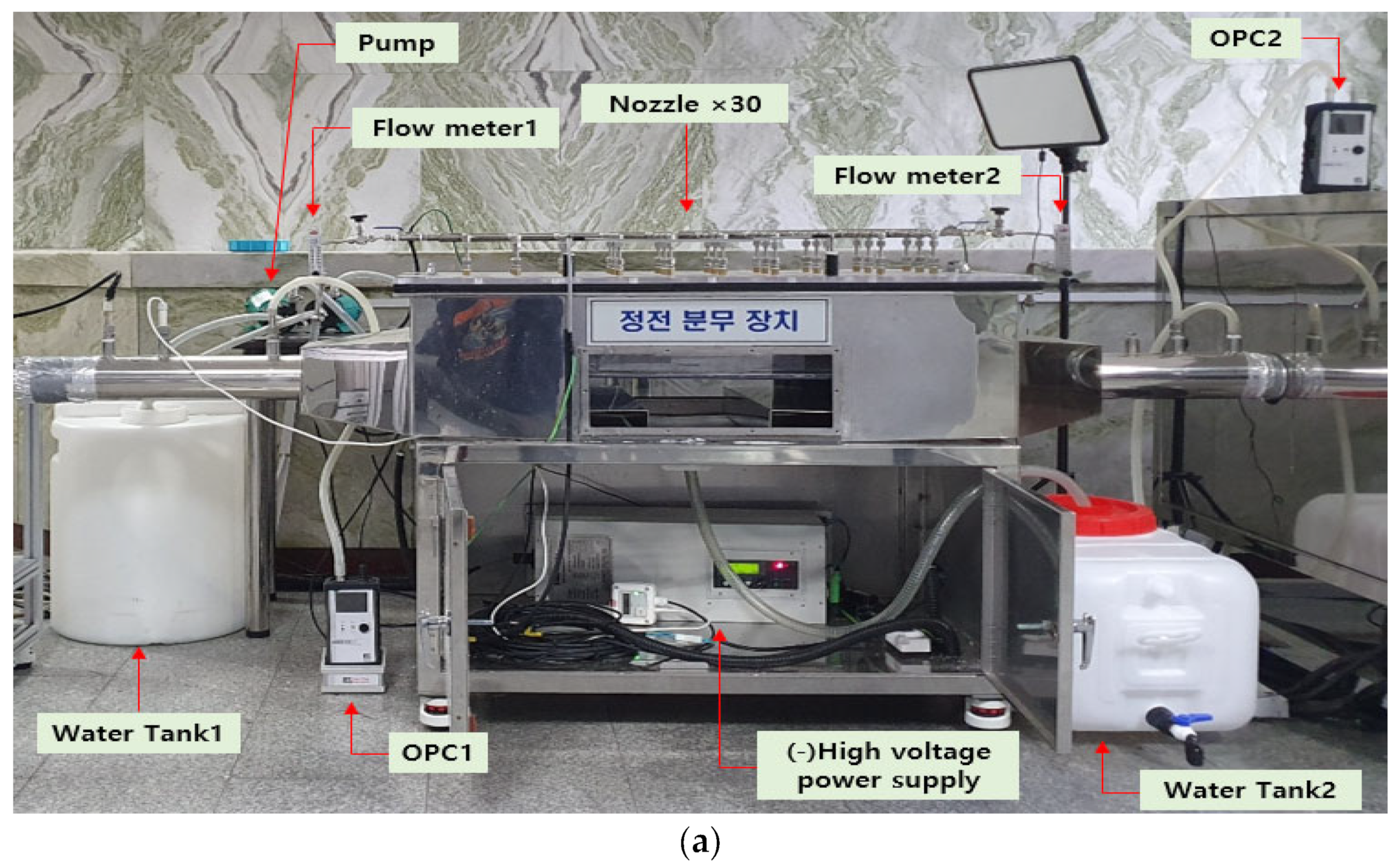
2.3. PM Generation Device

Figure 3 is a photograph of the constructed PM generation device. To ensure a stable supply of PM particles, an appropriate pressure was applied to a solution of KCl powder and diluted tap water using an air compressor (WSC-200-ST). The incoming solution was then filtered through silica gel blue, consisting mainly of silicon dioxide and with a particle size of 5~10 mesh, to generate the PM particles. KCL powder ranging in particle size from 0.3 μm to 10 μm is introduced with an air compressor and can most closely replicate the actual size of PM. Hence, particles similar to actual suspended PM and fine PM were generated and introduced at the entrance of the precipitator [27].

2.4. Electrostatic Spray-Based WESP Device

Figure 4 shows photographs of the manufactured electrostatic spray-based WESP device. A 100 L capacity water tank (Water tank 1) was installed to supply water, and a pump (PM-015NM) was used to supply water to the pipeline. A flow meter (RMA-42-SSV) installed in the pipeline controlled the flow of liquid, and a continuous water supply was provided to 30 nozzles installed on the precipitator’s ceiling. Additionally, a negative high voltage DC (direct current) supply device (PBS 7.5 (30 kV, 25 mA)) was installed to control the voltage within the range of 0–30 kV. A voltage of 1–7 kV was applied to the discharge electrode installed between the 30 nozzles supplying water and the collection electrode capturing PM. As shown in the figure, the collection electrode was installed below the discharge electrode, generating charged microdroplets and capturing PM through the collection electrode [28].

3. Principles of the Predictive Analysis Technique Based on the Ensemble Model

Figure 5 is an overall schematic diagram of the ML-based PM prediction model. To develop the PM collection efficiency prediction model using the collected data, the Python program-based Scikit-learn library was used [29]. The ML prediction models employed were kNN, RF, and decision tree (DT), which are commonly used ensemble models. Ensemble models are non-parametric ML methods that are less influenced by the relationship types between independent and dependent variables and the distribution of variables, and they can determine the relative importance or contribution of variables to the overall model [30]. Therefore, in this study, an optimal collection efficiency prediction model using ensemble models was proposed.

3.1. kNN (K-Nearest Neighbor)

The kNN model clusters data by utilizing the information of the k nearest neighbors. To apply the kNN algorithm, the k closest training data are selected according to the value of k and the distance measurement method, and the average of the output values is predicted. In the kNN algorithm, the Euclidean distance formula (Equation (1)) is used [31].

$$d\left(x, y\right)=\sqrt{{\displaystyle \sum }_i^n{\left(x_i-y_i\right)}^2},$$

(1)

where $x_i \mathrm{and} y_i$ are the x-coordinate and y-coordinate values, respectively.

3.2. DT(Decision Tree)

The DT method represents decision-making rules as a tree structure as shown in Figure 6 and classifies input data according to each branching question in order to make predictions. In DT training, data is classified from each branching node to the final node, and the data is classified into two or n steps depending on the depth value of the branch. At each node, the branching method involves finding the independent variable and threshold value with the largest information gain at the parent node and classifying the child nodes accordingly. The content of the information gain is represented in Equation (2) [32].

$$IG\left(D_p, f\right)=I\left(D_p\right)-{\displaystyle \sum }_{j=1}^n\frac{N_j}{N_p}I\left(D_j\right),$$

(2)

where $D_p$ is the dataset in the parent node, $D_j$ is the dataset in the j-th child node, $f$ is the feature value according to the branch, $I\left(D_p\right)$ is the impurity of $D_p$ data, $N_p$ is the number of data in $D_p$, $N_j$ is the number of data in the dataset, and $I\left(D_j\right)$ is the impurity of $D_j$.

This analysis method is advantageous because the prediction process is represented by inference rules based on the tree structure, increasing the computation speed compared to ANN, SVR, and regression models. Additionally, researchers can easily understand and explain the process.

3.3. RF(Random Forest)

RF is an ensemble model that aggregates multiple DT models, typically showing better prediction results than a single DT. It involves randomly sampling n pieces of data from a given dataset, creating several DTs, and determining the average prediction value based on the prediction results of each DT. The more DTs generated in the RF model, the better the performance of the prediction results [33,34].

The aforementioned ensemble model-based prediction models were tested using an 80% and 20% training and test datasets, respectively, and the results were compared with those of similar previous studies to verify the superiority of the models. The detailed settings of the model proposed in this study were determined with reference to existing studies on predicting PM in the atmosphere using similar data, and the values are presented in

Table 1. Ensemble model setting value.

ML Algorithms	Setting Value	Dataset	Reference
kNN	k = 3 (Euclidean distance)	PM 10 (Caribbean Area)	Plocoste et al. [35].
DT	Tree number ~100 Max depth	PM 10 (Caribbean Area)	Plocoste et al. [35].
RF	num. trees = 390, mtry = 16, min. node size = 4	PM 10, PM 2.5 (Atmosphere data)	Kim et al. [17].

.

3.4. K-Fold Cross-Validation

K-fold cross-validation is a common technique for evaluating the performance of a machine learning model. This method involves dividing the dataset into K equal-sized folds and conducting K iterations of model training and validation. During each iteration, K-1 folds are used for training and one fold is used for validation. The model’s performance is then evaluated based on the average score across all K iterations. By considering multiple iterations of model training and validation, this technique provides a more dependable estimate of model performance.

To optimize the ensemble model, we employed K-fold cross-validation to select the optimal hyperparameters. The hyperparameters considered included the number of individual models to combine and the weights assigned to each model. We employed K-fold cross-validation to assess the performance of the ensemble model for every combination of hyperparameters. The optimal hyperparameters were chosen based on the highest average performance across all K iterations. The K value in this paper was set to 100, and the hyperparameters were optimized through 100-fold cross-validation.

3.5. Model Performance Evaluation Metrics

3.5.1. R2 Score

R2 score is a performance evaluation metrics that assesses the correlation between the data applied to the regression model and the model. The R2 score ranges from 0 to 1, with values closer to 1 indicating a high correlation between the regression model and the applied data, and values closer to 0 indicating a low correlation. The formula for the R2 score is shown in Equation (3) [36].

$$R^2=1-\frac{{\left(T-P\right)}^2}{\sum {\left(T-A\right)}^2},$$

(3)

where $R$ is the coefficient of determination, $T$ is the target, $P$ is the predicted value, and $A$ is the average value.

3.5.2. MSE

MSE is the average of the squared differences between the predicted values and the actual values of the model. The higher the accuracy of the prediction model, the lower the MSE value. Also, since MSE squares the errors, the larger the error, the more heavily it is weighted, and the MSE value increases rapidly. The formula for MSE is shown in Equation (4) [37].

$$MSE=\frac{1}{N}{\displaystyle \sum }_{i=1}^N{\left(y_i-{\widehat{y}}_i\right)}^2,$$

(4)

where $y_i$ and ${\widehat{y}}_i$ are the actual and predicted values, respectively, and $N$ is the number of data points.

3.5.3. MAE

MAE is the average of the absolute differences between the predicted and actual values of the model, with lower values indicating a higher accuracy of the prediction model. Since MAE takes the absolute value of the errors, the size of the error is directly reflected, making it suitable for use when the size of the error is relatively large. The formula for MAE is shown in Equation (5) [38].

$$MAE=\frac{1}{N}{\displaystyle \sum }_{i=1}^N\left|y_i-{\widehat{y}}_i\right|,$$

(5)

where $y_i$ and ${\widehat{y}}_i$ are the actual and predicted values, respectively, and $N$ is the number of data points.

4. Experiments and Results

4.1. PLC-Based Dust Collection System Control Device and Real-Time Data Collection and Preprocessing

Figure 6 shows the experimental process of this study. First, the flow rate of one nozzle was set to 10 mL/min and the blower at the dust collector outlet was fixed at 30 Hz, and the voltage was increased from 1 to 7 kV at intervals of 1. The experiment was conducted for 150 min for each applied voltage, and sensor information within the PLC was collected in real-time every 6 s using the Python-based Pymodbus module. The collected data items include the input data and target data mentioned in Table 1. Second, mechanical error rates such as hardware loading from the sensor values collected in real-time were removed through preprocessing using the Python-based Pandas package, and dust collection efficiency was calculated using Equation (6) based on the collected PM inlet and outlet data [39]. Then, input data and target data were set, which are presented in

Table 2. Dataset information.

Input Data		Target Data
Inlet Temperature	Outlet Temperature	PM collection efficiency
Inlet Humidity	Outlet Humidity
Inlet PM 2.5	Outlet PM 2.5
Inlet PM 4	Outlet PM 4
Inlet PM 5	Outlet PM 5
Inlet PM 7	Outlet PM 7
Ozone	Voltage

.

Table 3. Experiment conditions of Wet electrostatic precipitators.

Item	Value
Solution	Tap water
Solution flow rate	10 [mL/min]
Nozzle inner diameter	0.55 [mm]
Voltage	1, 2, 3, 4, 5, 6, 7 kV
Measurement time by voltage	150 min
Data storage time unit	6 s

provides the detailed experimental conditions for PM collection. Finally, model training and evaluation were conducted to predict PM collection efficiency using kNN, DT, and RF models with the preprocessed data.

$$\eta =\left[1-\frac{C_o}{C_i}\right]\times 100\left(\%\right)$$

(6)

where $C_i$ is the PM concentration at the WESP inlet, and $C_o$ is the PM concentration at the WESP outlet.

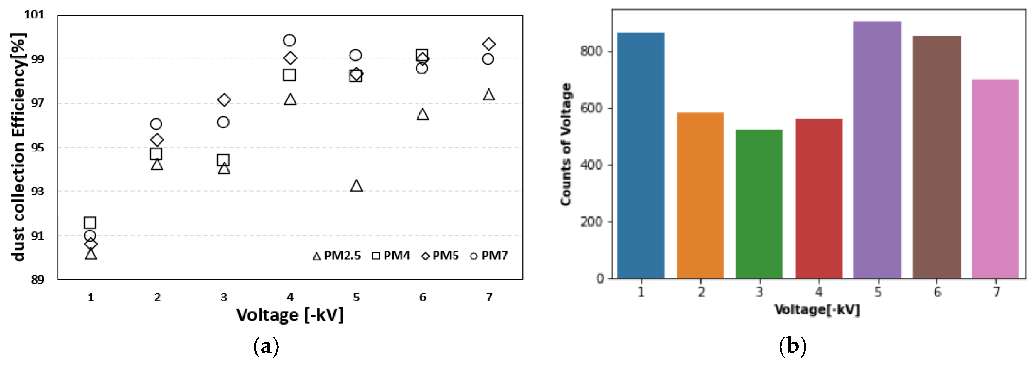
4.2. Dust Collector Experimental Results

Data was collected every 6 s for 150 min for each applied voltage, and the results of preprocessing for mechanical error rates such as hardware loading from the devices (OPC, etc.) and PM collection results by applied voltage are shown in Figure 7. Figure 7a shows that for PM 2.5, 4, 5, and 7, dust collection efficiency results of 90~95% were obtained in the range of 1–3 kV applied voltage, and from 4 kV onwards, the average dust collection efficiency was over 97%. Figure 7b shows that approximately 700–800 data points were collected as a result of data preprocessing. Consequently, this indicates that the PM collection efficiency tends to increase as the applied voltage increases, and about 5000 data points were collected through the experiment.

Figure 8 presents the trend of PM collection efficiency by PM size for different WESP operating conditions. Although Figure 7 demonstrates high performance in terms of the average PM collection efficiency, the distribution of actual data reveals a decrease in the dust collection efficiency with finer PM particles. Furthermore, the collected data exhibited highly dynamic characteristics, and the PM collection efficiency was found to vary significantly depending on the magnitude of the voltage applied to the WESP.

Figure 9 illustrates the variables that display fluctuations among the input values of inde-pendent variables, such as the PM count at the inlet and outlet of the WESP, the temperature and humidity values, the applied voltage, the ozone concentration, and the values of PM2.5, 4, 5, and 7 corresponding to the dependent variables. The figure suggests a correlation among these variables, where temperature, humidity, and ozone exhibit negative correlation coefficients, while the PM inlet and outlet concentrations and the applied voltage exhibit positive correlation coefficients. Therefore, the PM collection efficiency is substantially influenced by the operating conditions and the amount of inflow and PM collection.

Figure 10 illustrates the distribution of the PM values at the inlet and outlet of the WESP. The inlet value of PM2.5 exhibits significant variability, particularly with values distributed between 0 and 25,000,000 and rapid changes. Likewise, the PM outlet values are widely distributed and exhibit rapid changes. Hence, the dataset employed in this study is affected by multiple variables and interrelated intricately with each other. By utilizing a machine learning prediction model, it is possible to predict the PM collection efficiency by accounting for various variables necessary for the design and operation of the WESP.

In this study, we aimed to predict the PM collection efficiency of a WESP using various data, such as the inlet and outlet PM concentrations and applied voltage. These data are highly variable and exhibit rapid changes for each data point. To achieve this goal, we proposed the use of an ensemble series prediction model, which offers several advantages over traditional machine learning models. Ensemble models combine multiple models to increase accuracy, reduce bias, and improve robustness. Additionally, the ensemble model can handle complex and non-linear relationships between variables and can explain the interrelationships of the data used in this study. The ensemble model showed particularly high performance due to the complexity and variability of the data used, making it well-suited for the prediction of WESP PM collection efficiency.

4.3. Experimental Results of Dust Collection Efficiency Prediction Models

K-fold cross-validation is a powerful technique for evaluating machine learning model performance and selecting optimal hyperparameters. In this study, we demonstrated the use of K-fold cross-validation to optimize an ensemble prediction model, which resulted in improved accuracy and robustness.

4.3.1. kNN Model Prediction Results

Figure 11 shows the PM collection efficiency prediction results of the kNN model evaluated based on the test dataset. As the particle size of PM increases, the data is mainly distributed in the range of 90~100%, but the error between target data and predicted data increases. As a result, the kNN model’s predicted values tended to deviate more from the target as the particle size of PM increased during the prediction process.

4.3.2. DT Model Prediction Results

Figure 12 shows the PM collection efficiency prediction results of the DT model evaluated based on the test dataset. The error between target data and predicted data shows improved performance compared to the kNN model. Hence, the DT model demonstrates superior performance in predicting PM collection efficiency by reflecting various sensor values of the dust collector compared to the kNN model.

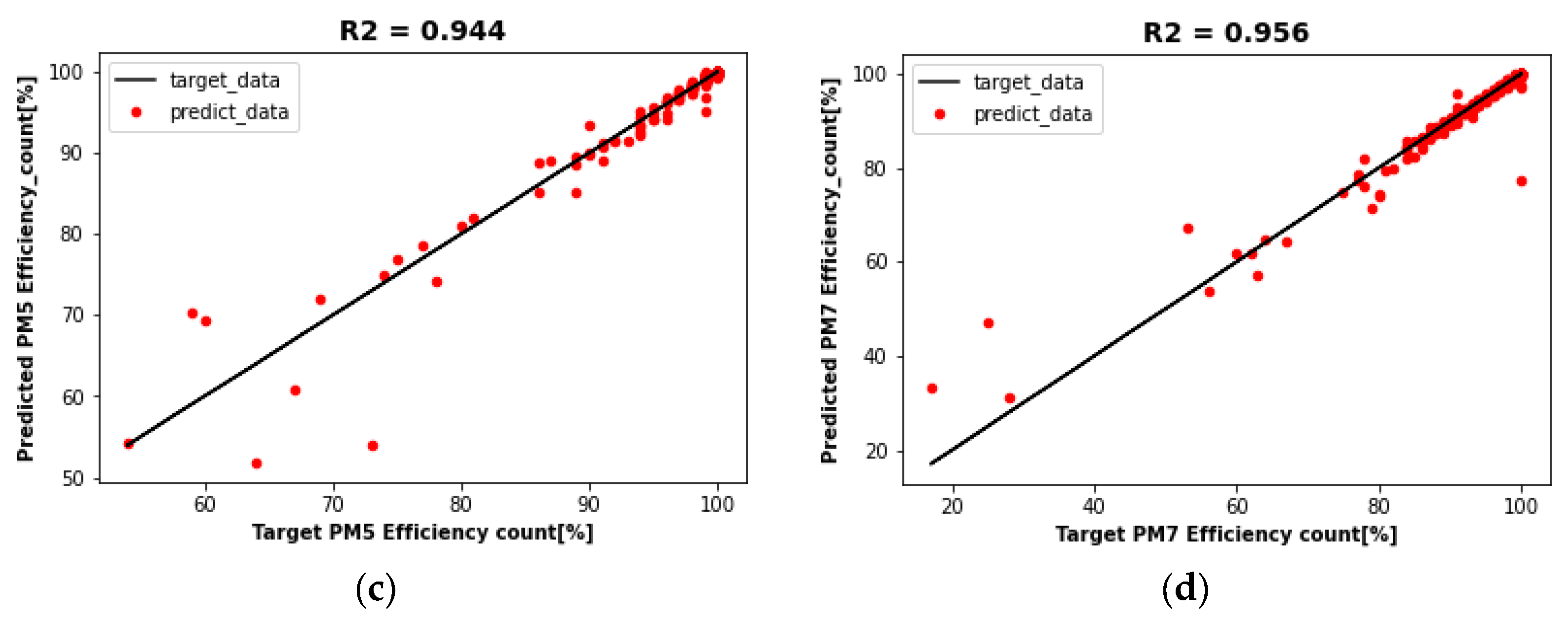
4.3.3. RF Model Prediction Results

Figure 13 shows the PM collection efficiency prediction results of the RF model for the test dataset. The RF model, which has a deeper algorithm depth and more complex structure than the DT model, showed superior performance in predicting PM collection efficiency compared to the DT model. Additionally, the error range of predicted values deviating from the target clearly decreased.

Table 4. Prediction model evaluation Result.

Target: Collection Efficiency	Model	R2-Score		MAE		MSE
		Train	Test	Train	Test	Train	Test
PM 2.5	kNN	0.955	0.905	0.383	0.710	4.834	10.772
	DT	0.998	0.921	0.046	0.460	0.173	8.887
	RF	0.993	0.942	0.120	0.380	0.741	6.548
PM 4	kNN	0.855	0.763	0.270	0.353	3.077	3.958
	DT	1.0	0.908	0.0	0.194	0.0	1.536
	RF	0.978	0.936	0.073	0.154	0.466	1.066
PM 5	kNN	0.661	0.705	0.508	0.618	7.529	4.266
	DT	1.0	0.872	0.0	0.205	0.0	1.850
	RF	0.972	0.944	0.075	0.613	0.154	0.815
PM 7	kNN	0.611	0.173	1.506	16.073	2.370	32.848
	DT	1.0	0.710	0.0	0.412	0.0	11.500
	RF	0.982	0.956	0.109	0.747	0.246	1.748

shows the performance evaluation results of the PM collection efficiency prediction models using kNN, DT, and RF. First, in the prediction results of dust collection efficiency for PM 2.5, 4, 5, and 7 evaluated in this study, the kNN model showed relatively large errors and low R2 score performance. Second, the DT model outperformed the kNN model but showed a tendency towards overfitting, as the evaluation result for the test dataset was lower than the training result for the training dataset. Finally, the RF model yielded the highest PM collection efficiency prediction performance with an R2 score of 0.93–0.95 for the test dataset.

5. Discussion and Comparison with Similar Works

This study proposes a machine learning-based model to predict the particulate matter (PM) collection efficiency of a wet electrostatic precipitator (WESP). While a WESP has many variables, including various flow rates, voltages, and fine dust concentrations, previous studies have only considered fixed conditions, such as the effective range of the electric field, internal space of the dust collector, and size of the dust collecting electrode. Variables that change in real-time, such as flow rate, voltage, and fine dust concentration, have not been adequately considered. Although the artificial neural network (ANN) model used in previous studies achieved an R2 score of 0.98, the random forest (RF) model proposed in this study achieved an excellent performance with an R2 score of 0.956, despite the difference in the number of data with large changes in real-time conditions, as shown in

Table 5. Comparison between proposed and existing model.

Algorithms	Model Evaluation Index	Parameter	Result	Reference
Hybrid model	R2	Inlet temperature[°C] Inlet concentration (g/m3) Rated migration velocity (ω)	0.933	Guo, Yishan, et al. [21].
ANN	R2, MSE	Inlet concentration (kg/m3) Gas flow rate (m3/s) Liquid flow rate (104 m3/s) Rotor speed (rpm) Particle size range (lm)	R2 = 0.962 MSE = 2.87	Li, Weiwei, et al. [22].
ANN	R2, MSE	gas temperature gas humidity gas velocity particle concentration	R2 = 0.9897 MSE = 0.27	Yang, Zhengda, et al. [23].
Random forest	R2, MSE, MAE	Inlet Temperature Outlet Temperature Inlet Humidity Outlet Humidity Inlet PM 2.5, 4, 5, 7 Outlet PM 2.5, 4, 5, 7 Ozone Voltage Blower	R2 = 0.956 MSE = 1.74	RF model [Ours]

. Therefore, the RF model shows excellent performance in predicting the fine dust collection efficiency, even in WESP with various fluctuating conditions. This model will greatly contribute to the production of fine dust collectors, detection of equipment aging, and WESP design and operation in the future.

6. Conclusions

This study proposed a new approach to PM collection efficiency prediction modeling using machine learning. We manufactured an actual PM collector to collect the dataset for the prediction modeling and conducted performance tests, reflecting the flow rate, voltage, flow velocity, and PM concentration of the dust collector. Ensemble model-based PM collection efficiency prediction models were developed for the sensor data collected from the dust collector under various variable conditions. According to the experimental results, the trained kNN model showed highly unfavorable prediction performance for new data in terms of error compared to the other models, and the DT model outperformed the kNN model but showed overfitting. On the other hand, the RF model yielded improved PM collection efficiency prediction performance for the test dataset compared to the kNN and DT models, with R2, MAE, and MSE scores of 0.956, 0.747, and 1.748, respectively, when the target was PM 7, and the error was substantially improved. Thus, we confirmed that the RF model showed the highest performance in predicting dust collection efficiency among the ensemble models. The RF model developed in this study is expected to contribute to various industrial fields in areas such as optimal WESP design reflecting the type and processing capacity of PM, stable operation, improvement of dust collector operating conditions, and diagnosis of equipment aging.

In future studies, we plan to analyze the structure of industrial WESPs to develop new electrode materials that can withstand high temperatures and corrosive environments. We aim to improve WESP performance by optimizing the electric field formed inside the dust collector to enhance PM collection efficiency. Additionally, we aim to develop an intelligent PM collector that can automatically control the applied voltage based on the PM concentration. This will maximize the collector’s performance by controlling its operating conditions through prediction of PM collection efficiency.

References

1. Santibáñez-Andrade, M.; Chirino, Y.I.; González-Ramírez, I.; Sánchez-Pérez, Y.; García-Cuellar, C.M. Deciphering the code between air pollution and disease: The effect of particulate matter on cancer hallmarks. Int. J. Mol. Sci. 2019, 21, 136. [Google Scholar] [CrossRef] [PubMed] [Green Version]
2. Carotenuto, C.; Di Natale, F.; Lancia, A. Wet electrostatic scrubbers for the abatement of submicronic particulate. Chem. Eng. J. 2010, 165, 35–45. [Google Scholar] [CrossRef]
3. Ritz, B.; Hoffmann, B.; Peters, A. The effects of fine dust, ozone, and nitrogen dioxide on health. Dtsch. Ärztebl. Int. 2019, 51–52, 881–886. [Google Scholar] [CrossRef] [PubMed]
4. Zhu, Y.; Gao, M.; Chen, M.; Shi, J.; Shangguan, W. Numerical simulation of capture process of fine particles in electrostatic precipitators under consideration of electrohydrodynamics flow. Powder Technol. 2019, 354, 653–675. [Google Scholar] [CrossRef]
5. Xu, X.; Zheng, C.; Yan, P.; Zhu, W.; Wang, Y.; Gao, X.; Luo, Z.; Ni, M.; Cen, K.; Ni, M.; et al. Effect of electrode configuration on particle collection in a high-temperature electrostatic precipitator. Sep. Purif. Technol. 2016, 166, 157–163. [Google Scholar] [CrossRef]
6. Jaworek, A.; Sobczyk, A.T.; Krupa, A.; Marchewicz, A.; Czech, T.; Śliwiński, L. Hybrid electrostatic filtration systems for fly ash particles emission control. A review. Sep. Purif. Technol. 2019, 213, 283–302. [Google Scholar] [CrossRef]
7. Yang, X.F.; Kang, Y.M.; Zhong, K. Effects of geometric parameters and electric indexes on the performance of laboratory-scale electrostatic precipitators. J. Hazard. Mater. 2009, 169, 941–947. [Google Scholar] [CrossRef]
8. Sobczyk, A.T.; Marchewicz, A.; Krupa, A.; Jaworek, A.; Czech, T.; Kluk, D.; Charchalis, A. Enhancement of collection efficiency for fly ash particles (PM 2.5) by unipolar agglomerator in two-stage electrostatic precipitator. Sep. Purif. Technol. 2017, 187, 91–101. [Google Scholar] [CrossRef]
9. Teng, C.; Fan, X.; Li, J. Effect of charged water drop atomization on particle removal performance in plate type wet electrostatic precipitator. J. Electrostat. 2020, 104, 103426. [Google Scholar] [CrossRef]
10. Wang, X.; You, C. Effects of thermophoresis, vapor, and water film on particle removal of electrostatic precipitator. J. Aerosol. Sci. 2013, 63, 1–9. [Google Scholar] [CrossRef]
11. Zhu, Y.; Wei, Z.; Yang, X.; Tao, S.; Zhang, Y.; Shangguan, W. Comprehensive control of PM 2.5 capture and ozone emission in two-stage electrostatic precipitators. Sci. Total Environ. 2023, 858, 159900. [Google Scholar] [CrossRef]
12. Su, L.; Du, Q.; Wang, Y.; Dong, H.; Gao, J.; Wang, M.; Dong, P. Purification characteristics of fine particulate matter treated by a self-flushing wet electrostatic precipitator equipped with a flexible electrode. J. Air Waste Manag. Assoc. 2018, 68, 725–736. [Google Scholar] [CrossRef]
13. Wu, H.; Pan, D.; Jiang, Y.; Huang, R.; Hong, G.; Yang, B.; Peng, Z.; Yang, L.; Yang, L. Improving the removal of fine particles from desulfurized flue gas by adding humid air. Fuel 2016, 184, 153–161. [Google Scholar] [CrossRef]
14. Xu, C.; Chang, J.; Meng, Z.; Wang, X.; Zhang, J.; Cui, L.; Ma, C. Wetting properties and performance test of modified rigid collector in wet electrostatic precipitators. J. Air Waste Manag. Assoc. 2016, 66, 1019–1030. [Google Scholar] [CrossRef] [Green Version]
15. Pan, D.; Gu, C.; Zhang, D.; Zeng, F. Removal characteristics of sulfuric acid aerosols in the wet electrostatic precipitator system. Energy Fuels 2019, 33, 7813–7818. [Google Scholar] [CrossRef]
16. Liu, T.; Xie, Y.; Su, S.; Wang, L.; Song, Y.; Chen, Y.; Xiang, J. Synergistic Removal Effects of Ultralow Emission Air Pollution Control Devices on Trace Elements in a Coal-Fired Power Plant. Energy Fuels 2022, 36, 2474–2487. [Google Scholar] [CrossRef]
17. Bozdağ, A.; Dokuz, Y.; Gökçek, Ö.B. Spatial prediction of PM10 concentration using machine learning algorithms in Ankara, Turkey. Environ. Pollut. 2020, 263, 114635. [Google Scholar] [CrossRef]
18. Kim, B.Y.; Lim, Y.K.; Cha, J.W. Short-term prediction of particulate matter. In Seoul, South Korea using tree-based machine learning algorithms. Atmos. Pollut. Res. 2022, 13, 101547. [Google Scholar] [CrossRef]
19. Iskandaryan, D.; Ramos, F.; Trilles, S. Air quality prediction in smart cities using machine learning technologies based on sensor data: A review. Appl. Sci. 2020, 10, 2401. [Google Scholar] [CrossRef] [Green Version]
20. Yang, G.; Lee, H.; Lee, G. A hybrid deep learning model to forecast particulate matter concentration levels in Seoul, South Korea. Atmosphere. 2020, 11, 348. [Google Scholar] [CrossRef] [Green Version]
21. Waseem, K.H.; Mushtaq, H.; Abid, F.; Abu-Mahfouz, A.M.; Shaikh, A.; Turan, M.; Rasheed, J. Forecasting of air quality using an optimized recurrent neural network. Processes 2022, 10, 2117. [Google Scholar] [CrossRef]
22. Guo, Y.; Zheng, C.; Xu, Z.; Yang, Z.; Weng, W.; Wang, Y.; Lu, J.; Gao, X.; Gao, X. Hybrid modeling scheme for PM concentration prediction of electrostatic precipitators. Powder Technol. 2018, 340, 163–172. [Google Scholar] [CrossRef]
23. Li, W.; Wu, X.; Jiao, W.; Qi, G.; Liu, Y. Modelling of dust removal in rotating packed bed using artificial neural networks (ANN). Appl. Therm. Eng. 2017, 112, 208–213. [Google Scholar] [CrossRef]
24. Yang, Z.; Cai, Y.; Li, Q.; Li, H.; Jiang, Y.; Lin, R.; Zheng, C.; Sun, D.; Gao, X.; Sun, D.; et al. Predicting particle collection performance of a wet electrostatic precipitator under varied conditions with artificial neural networks. Powder Technol. 2021, 377, 632–639. [Google Scholar] [CrossRef]
25. Choi, J.; Jeong, K.; Jung, H. Examining microdroplet characteristics of electrospray electric precipitation for direct and indirect voltage application methods. Int. J. Fire Sci. Eng. 2022, 36, 1–12. [Google Scholar] [CrossRef]
26. Mahmood, J.R.; Ali, R.S. Personal computer/programmable logic controller based variable frequency drive training platform using wxPython and PyModbus. Int. J. Electr. Comput. Eng. 2022, 12, 2088–8708. [Google Scholar]
27. Teng, C.; Li, J. Experimental study on particle removal of a wet electrostatic precipitator with atomization of charged water drops. Energy Fuels 2020, 34, 7257–7268. [Google Scholar] [CrossRef]
28. Kim, S.; Jung, M.; Choi, S.; Lee, J.; Lim, J.; Kim, M. Discharge current of water electrospray with electrical conductivity under high-voltage and high-flow-rate conditions. Exp. Therm. Fluid Sci. 2020, 118, 110151. [Google Scholar] [CrossRef]
29. Hackeling, G. Mastering Machine Learning with Scikit-Learn; Packt Publishing Ltd.: Birmingham, UK, 2017. [Google Scholar]
30. Aldrich, C.; Auret, L. Fault detection and diagnosis with random forest feature extraction and variable importance methods. IFAC Proc. Vol. 2010, 43, 79–86. [Google Scholar] [CrossRef]
31. Fathabadi, A.; Seyedian, S.M.; Malekian, A. Comparison of Bayesian, k-Nearest Neighbor and Gaussian process regression methods for quantifying uncertainty of suspended sediment concentration prediction. Sci. Total Environ. 2022, 818, 151760. [Google Scholar] [CrossRef]
32. Jong-wook, L.; Kim Young-Ho, B.B.-H.; Doo-seong, H. Obesity and metabolic syndrome data classification and feature importance analysis based on decision trees. Korean Inf. Process. Soc. Conf. Proc. 2021, 28, 880–883. [Google Scholar]
33. Shoar, S.; Chileshe, N.; Edwards, J.D. Machine learning-aided engineering services’ cost overruns prediction in high-rise residential building projects: Application of random forest regression. J. Build. Eng. 2022, 50, 104102. [Google Scholar] [CrossRef]
34. Kwak, S.; Kim, J.; Ding, H.; Xu, X.; Chen, R.; Guo, J.; Fu, H. Machine learning prediction of the mechanical properties of γ-TiAl alloys produced using random forest regression model. J. Mater. Res. Technol. 2022, 18, 520–530. [Google Scholar] [CrossRef]
35. Plocoste, T.; Laventure, S. Forecasting PM10 concentrations in the Caribbean area using machine learning models. Atmosphere 2023, 14, 134. [Google Scholar] [CrossRef]
36. Khan, M.A.; Khan, R.; Algarni, F.; Kumar, I.; Choudhary, A.; Srivastava, A. Performance evaluation of regression models for COVID-19: A statistical and predictive perspective. Ain Shams Eng. J. 2022, 13, 101574. [Google Scholar] [CrossRef]
37. Pattana-Anake, V.; Joseph, F.J.J. Hyper parameter optimization of stack LSTM based regression for PM 2.5 data in Bangkok. In Proceedings of the 7th International Conference on Business and Industrial Research (ICBIR), Bangkok, Thailand, 19–20 May 2022; IEEE Publications: New York, NY, USA, 2022; Volume 2022, pp. 13–17. [Google Scholar] [CrossRef]
38. Jiang, Y.; Xia, T.; Wang, D.; Fang, X.; Xi, L. Adversarial regressive domain adaptation approach for infrared thermography-based unsupervised remaining useful life prediction. IEEE Trans. Ind. Inform. 2022, 18, 7219–7229. [Google Scholar] [CrossRef]
39. Xiaochuan, L.; Mingrui, Z.; Yefeng, J.; Li, W.; Xinli, Z.; Xi, C.; Haoyu, B.; Xianming, D.; Xianming, D. Air curtain dust-collecting technology: Investigation of factors affecting dust control performance of air curtains in the developed transshipment system for soybean clearance based on numerical simulation. Powder Technol. 2022, 396, 59–67. [Google Scholar] [CrossRef]
Figure 1. Conceptual diagram of principles of indirect-charging electrostatic spraying.
Electronics 12 02579 g001
Figure 2. Schematic diagram of PM collection system.
Electronics 12 02579 g002
Figure 3. Actual PM generator.
Electronics 12 02579 g003
Figure 4. Electrostatic spray-based WESP device (a): Front view of the precipitator, (b): Top view of the precipitator.
Electronics 12 02579 g004aElectronics 12 02579 g004b
Figure 5. An overall schematic diagram of the ML-based PM prediction model.
Electronics 12 02579 g005
Figure 6. Development process of PM 2.5 prediction models.
Electronics 12 02579 g006
Figure 7. WESP dust collection results by applied voltage. (a) PM collection efficiency by applied voltage; (b) Number of data by applied voltage.
Electronics 12 02579 g007
Figure 8. Distribution of PM collection efficiency by applied voltage. (a) PM 2.5 efficiency distribution; (b) PM 4 efficiency distribution; (c) PM 5 efficiency distribution; (d) PM 7 efficiency distribution.
Electronics 12 02579 g008
Figure 9. Correlation of data variables.
Electronics 12 02579 g009
Figure 10. WESP inlet, outlet PM distribution. (a) Inlet PM distribution; (b) Outlet PM distribution.
Electronics 12 02579 g010
Figure 11. PM collection efficiency prediction results (kNN model). (a) PM 2.5 efficiency prediction; (b) PM 4 efficiency prediction; (c) PM 5 efficiency prediction; (d) PM 7 efficiency prediction.
Electronics 12 02579 g011
Figure 12. PM collection efficiency prediction results (DT model). (a) PM 2.5 efficiency prediction; (b) PM 4 efficiency prediction; (c) PM 5 efficiency prediction; (d) PM 7 efficiency prediction.
Electronics 12 02579 g012
Figure 13. PM collection efficiency prediction results (RF model). (a) PM 2.5 efficiency prediction; (b) PM 4 efficiency prediction; (c) PM 5 efficiency prediction; (d) PM 7 efficiency prediction.
Electronics 12 02579 g013aElectronics 12 02579 g013b