Study on the Selection Method of Federated Learning Clients for Smart Manufacturing

Abstract

Artificial intelligence technology in the context of smart manufacturing uses manufacturing data to enable the automatic detection, classification, and identification of products in the production process, reducing production costs and human consumption, thereby improving production efficiency and product quality. Federated learning enables the distributed implementation of AI technologies, keeping data local to avoid privacy leaks. However, data heterogeneity factors have an impact on federated learning in a manufacturing context, and this paper proposes a customer degree selection method based on model parameter variation. The method relies on transmitting the local model changes in the participants to reflect the data characteristics, calculates the model similarity of the participants using graph theory and similarity, and uses the Top-K mechanism to filter the original participant set through the similarity scores of graph nodes to reduce the influence of heterogeneity factors in the participant set and maximize the training effect and accuracy of federated learning. The effectiveness of this method was verified by using the Dirichlet distribution to perform non-IID data partitioning on the power system attack dataset and the hard disk fault detection dataset.

1. Introduction

As manufacturing becomes an increasingly significant part of economic impact, modern manufacturing is creating new products or services with characteristics such as customization, adaptability, and reliability at an unprecedented scale. These new products or services have become an integral part of our daily lives through the transformation of fixed and cumbersome traditional manufacturing into rapid, customized additive manufacturing [1] and digital and intelligent smart manufacturing. While the functional and scalable nature of the product or service makes manufacturing systems increasingly complex, Industry 4.0 is driving manufacturing to become a new generation of cyber-physical systems, moving towards enabling cyber-enabled smart manufacturing [2]. Industrial infrastructure, smart manufacturing technologies, and the large-scale digitization of assets and processes across industries are driving manufacturing into a new era. The drive and construction of smart manufacturing systems requires the digitization of modern manufacturing through data-driven analytics tools such as artificial intelligence, machine learning, digital twins, cloud computing, and big data analytics [3,4,5]. These rapidly evolving technologies, coupled with the exponential growth of manufacturing data, have enabled data-hungry artificial intelligence and machine learning to develop at an unprecedented scale [6]. The distributed nature of modern industrial IoT systems and traditional centralized machine learning techniques pose a direct threat to data sharing. Take, for example, the task of target identification and classification in smart manufacturing, which requires the upload of raw data collected by different cameras to a centralized server (e.g., a cloud server), which can lead to the potential leakage of confidential information (e.g., the product being manufactured or personal information collected) during transmission. The concept of federated learning has recently been introduced to facilitate knowledge sharing between multiple smart end devices while protecting data privacy by avoiding the sharing of raw data between the end devices and the central server. In a federated learning-based smart manufacturing system, multiple cameras can collect product images and train a local model individually. By not transferring the raw data, only the local model parameters are encrypted and uploaded to a central server to form a global model. By combining multiple local models, the global model is expected to provide more generalized and accurate predictions.

Unlike general distributed collaborative modelling scenarios in data center-based environments, federated learning in smart manufacturing scenarios usually faces complex computing environments with heterogeneity, whose heterogeneity can adversely affect the effectiveness of models in federated scenarios. The existing approaches to deal with data heterogeneity factors often have many constraints and limitations or lack certain generality for complex smart manufacturing scenarios that cannot balance computational overhead, accuracy assurance, etc. For example, the FedAvg algorithm uses a random selection strategy to filter clients in order to reduce the computational overhead, but this random selection of clients can exacerbate the adverse effects of data heterogeneity [7]. Therefore, this paper considers the industrial environment oriented towards smart manufacturing and federated learning to face the problem of data heterogeneity according to the business scenario and proposes a novel client selection method based on the variation in model parameters to filter the initial client set; in summary, the contributions of this paper are as follows:

The impact of manufacturing data on the performance of federated learning is verified through experimental analysis.

To reduce the impact of data heterogeneity, a client selection method based on model parameter variation is designed to select a more similar set of clients using graph theory and similarity calculations to reduce the model differences between clients and each other.

Experiments are conducted to classify different manufacturing data using Dirichlet distribution to verify the effectiveness of the method used in this paper.

2. Related Work

Since its introduction, federated learning has gained widespread interest and has been used in many scenarios. A major advantage of federated learning is that it addresses the problem of data aggregation and therefore enables the design and training of cross-device machine learning models and algorithms across different industries and sectors. In particular, applying machine learning models to mobile, federated learning has demonstrated excellent training capabilities and robustness [8]. In addition, federated learning can greatly improve the performance of machine learning models and algorithms for some users, who often cannot provide enough personal data to build accurate local models. However, federated learning focuses on learning the local data of all participating users (devices) through a distributed architecture to obtain high-quality global models, and device performance differences do not capture the personal information of each device, resulting in degraded inference or classification performance [9]. In addition, traditional federated learning requires all participating devices to agree on a common model for collaborative training, which is impractical in the context of real, complex IoT applications. The FedAvg algorithm [10] demonstrates that random customer selection is effective when all customers are available and adequately trained, but is not optimized for the non-IID problem, resulting in low model accuracy. To improve the performance when federated with heterogeneous data, Li et al. [11] proposed FedProx, which introduces a proximal term to restrict local updates to more closely resemble the global model. Traditional federated learning requires all participating devices to agree on a common model for collaborative training, which is impractical in realistic and complex IoT application environments. Nishio et al. [12] first proposed a FedCS federated learning client selection algorithm for edge devices based on system heterogeneity, the main idea of which is that the client sends its resource information (communication status, computing power and resource size, etc.) to the server, which estimates the time required for the update and upload steps based on the received information and determines which users participate in the training. However, this method ignores the effect of data heterogeneity and cannot be optimized by selection methods for data heterogeneity. In the FedSim algorithm [13], pairs of client similarities are used for clustering, but it makes full use of the algorithm’s local model parameters’ client and uses clustering as a post-federated learning processing technique, whereas we only use some of the local model parameters for client selection at one time. Wang et al. [14] proposed a new federated learning scheme that uses cosine similarity to remove invalid models and clusters devices by vectorizing local and global model parameters. Our proposed method makes it simple to compute similarity using local model parameters and requires less computational and communication power.

In summary, the research and analysis verifies that random client selection can have an impact on federated learning, and that studies that generally address a particular aspect ignore information about the impact of the relationships between clients. This paper therefore focuses on client selection methods that consider the similarities between all clients and methods that improve the efficiency and accuracy of federated learning convergence in non-IID scenarios.

3. Background

3.1. FL Optimization Objectives

Federated learning is a distributed machine learning framework that enables participating users to collaboratively train a shared global model on a virtual collection of local data, without having to move the data out of the local environment.

Federated learning can be defined as follows. Assume that there are N data holders in the federated learning process; all of the data holders can be represented by $C=\left\{c_1,c_2,\dots ,c_N\right\}(∥C∥=N)$. Before they are federated for modelling, the total set of data in the system is defined as S, i.e., $S=(s_1,s_2,\dots ,s_N\}$, which contains a total data size of $D={\sum }_{n=1}^N{D}_n$. After these data holders have been federated, with each holding a local dataset $s_n\left(n\in \left[1,N\right]\right)$ of size $D_n$, the resulting model can be defined as Modelfed, and the performance of the model can then be expressed in terms of model accuracy $Performanc{e}_{fed}$, and throughout the federated learning process. Each data holder $c_i$ does not share its data directly with other holders. Federated learning overcomes the privacy and communication challenges compared to centralized learning by eliminating the need to aggregate all datasets and only using local machine learning or deep learning models to learn from the dispersed data. The model obtained by aggregating data for centralized learning, as opposed to federated learning, can be defined as $Mode{l}_{cent}$, and the performance accuracy of the same obtained model is $Performanc{e}_{cent}$. Making the gap between the $Performanc{e}_{fed}$ of $Mode{l}_{fed}$ and the $Performanc{e}_{cent}$ of the model $Mode{l}_{cent}$ sufficiently small is the optimization goal of federated learning, as shown in Equation (1):

$$\left|Performanc{e}_{fed}-Performanc{e}_{cent}\right|<\delta$$

(1)

$\delta$ is an arbitrarily small positive number. Because of the different data distributions held by data owners in real-world scenarios and the errors that arise from many calculations for communication problems or to ensure model efficiency, this is the difference between federated and centralized learning, and minimizing errors and improving accuracy is where federated learning algorithms excel.

The main steps in federated learning can be divided into four parts: local training, passing updates, model aggregation, and gaining benefits. Figure 1 shows the structure of a federated learning framework in which multiple data-holding users are trained locally by holding data to obtain a local model. The function of the central server in federated learning is to coordinate a federated learning process consisting of multiple training rounds, and the server passes the current global model to the data holders at the beginning of each training round. Therefore, after receiving the passed updates, the central server aggregates the trained local models and updates them to the local models of each data-holding user to gain a better global model.

For local model training, the weights $\omega$ of the model obey a certain real number space and the loss error obtained when fitting to the $i-th$ data sample point $\left(X_i,Y_j\right)$ is shown in Equation (2):

$$f_i\left(\omega \right)=\ell \left(X_i,Y_j;\omega \right)$$

(2)

When training the model, an optimal algorithm is used to continuously optimize this loss function in order to obtain the best model parameters, and the model training, as an optimization problem, is defined by the optimization objective, as shown in Equation (3):

$$\underset{w}{min}f\left(\omega \right)={\displaystyle \frac{1}{D}}\sum _{n=1}^D{f}_i\left(\omega \right)$$

(3)

Thus, for each federated learning client, the data it holds can be viewed as a subset of the overall dataset, and the loss it causes is shown in Equation (4):

$$F_n\left(\omega \right)={\displaystyle \frac{1}{D_n}}\sum _{i\in S_n}{f}_i\left(\omega \right)$$

(4)

Thus, the federated learning global optimization objective in Equation (3) can be rewritten using Equation (5), as follows:

$$\underset{\omega }{min}f\left(\omega \right)=\sum _{n=1}^N{\displaystyle \frac{D_n}{D}}·F_n\left(\omega \right)$$

(5)

3.2. Design Motivation

The federated training of clients leads to biased aggregation models due to the differences between local models caused by the heterogeneous data in the manufacturing industry. In order to obtain better aggregation models, a combination of clients with high data correlation and low variability between clients needs to be constructed; this will result in a better similarity between the trained models, and the resulting federated learning aggregation models will be less affected by bias in the data distribution. Since the assumption in federated learning is that the data are not local, only the model information and parameters can be passed on. Client-side local model training yields iterative parameter changes that reflect the impact of the data characteristics on model performance. Compared to Euclidean distance, which has the problem of dimensional catastrophe in high-dimensional space, cosine similarity is more applicable than Euclidean distance when dealing with high-dimensional data; thus, calculating the similarity between federated learning clients through cosine similarity has lower computational complexity. The relationship between nodes and edges in graph theory can be mapped to the connection between all clients of federated learning, and the graph model built by using clients as nodes can effectively associate the clients and facilitate the relational operation between them.

4. Algorithm Design

This section first presents an analytical introduction to the impact of manufacturing data heterogeneity on federated learning and then describes the client selection method designed in this paper.

4.1. Data Heterogeneity Analysis

Previously, both machine learning and deep learning held the fundamental assumption that data were uniformly and homogeneously distributed. In contrast, actual industrial scenarios produce data that are often heterogeneous and uneven. In the context of smart manufacturing, there are two main factors of data heterogeneity that affect the performance of federated learning models: heterogeneity due to differences in the distribution of client data and unevenness in the number of samples. The impact in terms of their data heterogeneity is mainly due to the local data distribution bias caused by differences in the amount of sample data in certain categories. Figure 2 illustrates the distribution differences due to the data heterogeneity factors of participants in federated learning.

In federated learning in the context of smart manufacturing, the distribution of training datasets kept by each computing node usually does not satisfy the assumption of independent homogeneous distribution, which is very different from the traditional distributed machine learning environment. In fact, the heterogeneity of data distribution in federated learning can be seen as a situation where the distribution of data across clients does not meet the independent homogeneous distribution condition. FedAvg, a classical algorithm in federated learning, presents a key problem when faced with data heterogeneity: when the global model is optimized using different local objectives, the average of the generated client updates (server updates) will be far from the true global optimum. The cause of this inconsistency is known as client drift [15] and is shown in Figure 3.

4.2. Client Selection Method Based on Variations in Model Parameters

The key to the client selection algorithm based on model parameter changes is similarity calculation and graph theory. This section establishes a clear client selection algorithm based on cosine similarity and graph theory. The basic idea of this algorithm is that, in compliance with the setting that federated learning only passes parameters but not data, the data characteristics are reflected by passing the client model parameter changes, and a more accurate similarity calculation is performed by the server on the parameter information using graph theory and similarity, allowing for each client to search for other clients that are more similar in terms of data distribution and to interact with each client more, helping to filter for a larger and more similar form of training. This helps to filter larger and more similar training data to avoid skewing the model, thus improving the training effectiveness of the model.

The client selection algorithm based on the variation in model parameters is divided into a total of four steps, as shown in Figure 4, as follows:

Step 1: Server information collection. In order to assess the similarities between clients, it is intuitive to collect data information from each client; however, subject to the constraint that federated learning only passes parameters and not data, relying on the collection of model parameter changes to reflect data information naturally incorporates our solution for client similarity measurements. The process of picking a collection of clients first requires the collection of client information, and at this stage, the aggregation server must obtain information on the model transformations of the clients. The client’s local model is iterated locally via Equation (6), and the difference in model parameters between the first and last local iteration of client c’s model parameter ${\omega }^c$ is denoted as $\widehat{{\omega }^c}$, which represents the parameter change in client c’s model parameter ${\omega }^c$ that occurs between e epochs. The model parameter changes $\left\{\widehat{{\omega }^1},\widehat{{\omega }^2},\widehat{{\omega }^3},\dots ,\widehat{{\omega }^n}\right\}$ for N clients are obtained through local training, performed by the clients in parallel, and the aggregation server collects this information.

$${\omega }_t^k={\omega }_{t-1}-\eta ·\nabla L\left({\omega }_{t-1}\right)$$

(6)

Step 2: Client-side construction of the undirected graph. Since similarity calculations can only reflect the relationship of a given vector, but clients in the manufacturing industry have complex associations, direct similarity calculations regarding the changes in client model parameters collected in Step 1 cannot take more complex relationships into account. The relationship between nodes and edges in graph theory can help to uncover more complex connections, so this paper uses the construction of undirected graphs with clients as nodes, combined with similarity calculations to improve the accuracy and interpretability of the calculations. The graph is constructed using the total number of clients, N, as the number of nodes in the undirected graph, with each node representing each client $C=\left\{c_1,c_2,\dots ,c_n\right\}$ in federated learning. A complete graph G is constructed, with edges corresponding to different nodes in the graph. The aggregation server processes the information that was collected about the changes in the model parameters $\widehat{\omega }$. The parameter changes represent the node values of each client separately in the undirected graph.

Step 3: Similarity and graph node degree calculation. The node values derived from Step 2 for each client are used to calculate the weights $cos{\theta }_{ij}(i\ne j,i,j\in n)$ of the edges between the client nodes using the multi-dimensional cosine similarity in Formula (7), which maps the model similarity between two nodes, i.e., two clients, and can be stored in the adjacency matrix, as shown in Equation (8). The undirected complete graph G generated by Step 2 is formed into a weighted undirected complete graph $\tilde{G}$ based on the weights $cos{\theta }_{ij}$ between each node, and the weights between the node and all its connected nodes are calculated using Equation (9) to obtain the degree $d_i$ of the node and indicate the strength or importance of the connection between the node and other nodes.

$$cos\theta ={\displaystyle \frac{{\Sigma }_1^n\left(A_i\times B_i\right)}{\sqrt{{\Sigma }_1^n{A}_i^2}+\sqrt{{\Sigma }_1^n{B}_i^2}}}$$

(7)

$$\left[\begin{array}{ccc}0& \dots & cos{\theta }_{1n}\\ ⋮& ⋮& ⋮\\ cos{\theta }_{n1}& \dots & 0\end{array}\right]$$

(8)

$$d_i=\left(cos{\theta }_{i1}+\dots +cos{\theta }_{in}\right)$$

(9)

Step 4: Top-K output client set. Statistics of the degree of each node in the weighted undirected complete graph, according to the weights of the degree, as in Step 4 in Figure 4. Apply the Top-K selection mechanism, set the size of the number of output sets according to the hyperparameters $\beta \in \left(0,1\right)$ to filter the original client, and select the client set $C_K\left(C_K\subset C\right)$ with closer similarity, where K indicates the number of sets $C_K$, with $K=\beta ·N$, which can be realized according to Formula (10) in the original client set C for selection.

$$C_k\stackrel{K,\tilde{G}}{\leftarrow }C$$

(10)

5. Experimental Setup and Results

5.1. Data Acquisition

A total of two means of manufacturing classified data were used for the experiments in this paper, as follows. The power system attack dataset [16] was provided by Mississippi State University, which was generated by simulating a power system with complex electronic equipment and monitoring system interaction. The power system structure is shown in Figure 5. G1 and G2 are power generators, IED1 through IED4 are Intelligent Electronic Devices (IEDs) that can switch the breakers (R1 through R4) on or off, and the substation network is responsible for controlling the relays and transmitting information. The IEDs use a distance protection scheme, which trips the breaker on detected faults, regardless of whether they are valid or faked, since they have no internal validation to detect the difference. The monitoring system records not only the physical information about the operation of each of the four relays, but also the panel, alarm, and relay log information of the corresponding relays. In addition to the normal operating outage events of this power system, as the substation is connected via the network, attackers can rely on the network to inject attack commands and disguise the system outage, thus disrupting the staff and ensuring that they are not able to identify the state of the outage event being attacked, which disrupts the normal operation of the system and causes the industrial data records to be untrue. The dataset contains 37 power system event scenarios, and the dichotomous dataset is a classification of the 37 event scenarios into attack scenarios (28) and normal events (9). Each data sample contains 128 feature messages, of which 116 feature messages consist of four phasor measurement units (PMUs); each PMU contains 29 types of measurement. The index of each column is in the form of ‘R#-Signal Reference’ that indicates a type of measurement from a PMU, specified by ‘R#’. For example, ‘R1-PA1:VH’ means the Phase A voltage phase angle measured by PMU IED1. After that, there are 12 columns for control panel information, Snort alerts, and relay logs of the 4 PMU/relay.

The Hard Drive Failure Detection Dataset [17] is available in BackBlaze’s data center and the data collect the S.M.A.R.T. attributes of the ST4000DM000 model hard drive, a self-diagnostic technique that can be used to predict hard drive failures. This dataset contains information including the drive’s SMART attributes, as well as characteristics such as model, serial number, date, and capacity. After the dataset has been filtered and processed for valid information, the hard drive failure detection dataset has a feature count of 11, with two states of “normal” and “failed” hard drives.

5.2. Dirichlet Divides Heterogeneous Data

The Dirichlet distribution is a common multidimensional continuous distribution that plays an important role in probability statistics and is usually denoted by $Dir\left(\alpha \right)$. Its parameters are controlled by the positive real vector $\alpha$, and the distribution of this vector is also a probability distribution, so the term “distribution of probability distributions” can also be used to describe the Dirichlet distribution. For the federated learning experimental scenario, the IID dataset is sampled according to the Dirichlet distribution to obtain the non-IID dataset. If there are N category labels and K clients, the samples of each category label need to be divided on different clients in different proportions. Let matrix $X\in {\mathbb{R}}^{K\ast N}$ be the category label distribution matrix, whose row vector $X_N\in {\mathbb{R}}^K$ represents the probability distribution vector of category N on different clients (each dimension represents the proportion of samples of category N divided on different clients), and this random vector is sampled from the Dirichlet distribution. Therefore, the local training datasets held by each participant can be obtained as non-IID datasets by sampling the source datasets with the same probability as the probability of the parameter vector $q(q_i\ge 0,i\in \left[1,N\right])$. A sample of participant non-IID data can be generated by sampling the probabilities of the Dirichlet distribution corresponding to Equation (11):

$$q\sim Dir\left(\alpha p\right)$$

(11)

By varying the values of the parameters, different participant local datasets can be sampled according to the probability distribution of Equation (11). At $\alpha \to 0$, the local data sample set for each participant is simply a random sample from a class of samples. At $\alpha \to \infty$, the prior distribution of the source dataset coincides with the distribution of the local data generated by each participant. That is, the smaller the $\alpha$, the more dispersed the distribution; the larger the $\alpha$, the more that distribution tends to be uniformly distributed. Therefore, if the prior distribution is IID, the distribution q becomes increasingly different as $\alpha$ becomes smaller; as $\alpha$ increases, the distribution q becomes increasingly similar.

The parameter $\alpha$ can have an impact on the range of bias in data generation. Taking the manufacturing data power system attack dataset [15] as an example, the $client\_id$ axis in Figure 6 indicates the ID of each participant in federated learning, the $label$ axis indicates the label type of each participant’s sample set, and the $number$ indicates the number of data samples in the corresponding category for each participant. In Figure 6a, when $\alpha$ is set to 1, the data distribution of each participant is heavily skewed, with large differences in the number of samples for different participants in the same category, and the distribution of categories among different participants is also different. When $\alpha$ is taken as 10 in Figure 6c, the data distribution across participants is skewed, but the variation is small and participants still hold different numbers of category labels. For $\alpha$ value of 50 in Figure 6d, the data distribution across participants in this scenario is slightly skewed and the variation between participants is small, close to the distribution state of the IID dataset.

5.3. Experimental Configuration and Evaluation Indicators

For the experimental environment, a mobile workstation was used to simulate the experiments, which was configured with a 7th generation Intel processor i7-11850H at 2.5 GHz, a graphics card of Nvidia GTX 3080, and an operating system of Windows 10 64-bit. The development tools used were Python 3.7, the neural network library Keras, and the experiments were programmed using a single machine system model federated learning training process. For evaluation metrics, the models are evaluated in this paper on both datasets using Accuracy, which is calculated as follows:

$$Accuracy={\displaystyle \frac{TP+TN}{TP+FP+TN+FN}}$$

(12)

where TP, TN, FP, and FN denote true examples, true counterexamples, false positive examples, and false counterexamples, respectively.

5.4. Experimenting with Data Heterogeneity in Smart Manufacturing

In this section, two separate experiments are conducted to better explore the effect of manufacturing data on FedAvg. Firstly, an experimental analysis of the effect of IID and non-IID data on FedAvg under different parameters is presented, and then the effect of different degrees of distribution on FedAvg under the non-IID setting is verified.

(1) Effect of IID and Non-IID data on FedAvg

IID data are a strong assumption in machine learning, especially since manufacturing data tend to exist as non-independent identical distributions. To verify the fact that the federated learning algorithm has significant accuracy degradation on non-IID manufacturing data, this section conducts comparative experiments on the power system attack dataset [15], which is described in detail in Section 4. The experiments are set up with five federated learning clients, and non-IID is partitioned according to a Dirichlet distribution with hyperparameter $\alpha =1$. The number of federated global communications was set to 50, the classical FedAvg algorithm was used as the federated learning algorithm, and the MLP model was chosen for the network model. Three parameter settings were used experimentally for non-IID, as shown in

Table 1. Experimental setup for IID and non-IID.

Set Number	Data Distribution	BatchSize $\left(\mathit{B}\right)$	Epoch $\left(\mathit{E}\right)$
0	IID	10	1
1	Non-IID	10	1
2	Non-IID	10	5
3	Non-IID	20	1

.

The specific experimental results are shown in Figure 7, where Figure 7a shows the accuracy variation graphs based on FedAvg using the MLP local model on the power system attack dataset, and Figure 7b shows its loss degradation variation. There are three different non-IID parameter settings in Figure 7a, with both ordinal numbers 1 and 3 showing some reduction in accuracy compared to the independent identically distributed setting of ordinal number 0, with an average drop in accuracy of 6.12% and 5.98% in the global iteration, respectively. Although the accuracy of ordinal number 2 is higher than the IID data in some of the communication rounds, its training process becomes more oscillating, with an average reduction in accuracy of 6.03% compared to the IID setting in the global iteration. The non-IID data in Figure 7b showed a higher rate of decline than the IID data setting for all three parameter settings. Observing the curve changes, it can be seen that the IID data with the ordinal number 0 setting showed a stable loss decline with little fluctuation. For the non-IID data, the loss variation curves for each parameter setting fluctuated to varying degrees, with the largest oscillation in loss decline being noted for the No. 2 setting. The above experimental results can be interpreted as follows. Due to the different distributions of the non-IID data samples, the increased dispersion of data features may cause some samples to appear more frequently and some samples to appear less frequently. The model does not balance the contribution of each sample well during training and the features are not sufficiently learned, resulting in overfitting of the model to the samples that occur more frequently and large differences between local model parameters, causing large fluctuations in accuracy and loss variation.

(2) Effect of different degrees of Non-IID data on FedAvg

In addition, we also verified the effect of different degrees of non-independent identically distributed data on FedAvg by varying the hyperparameters $\alpha$ dividing different non-IID data experiments with Dirichlet. A total of four different degrees of non-independent identically distributed data were set up for the experiments, i.e., the hyperparameters $\alpha$ were set to 1, 5, 10, and 50, respectively, and the data distribution is illustrated in Figure 6, where BatchSize was set to 10 and epoch to 1.

The performance of the FedAvg algorithm for different data distributions under the power system attack dataset is shown in Figure 8. The rising variation in the accuracy of FedAvg is illustrated in Figure 8a. As the parameter $\alpha$ becomes larger, the more homogeneously the data tend to become distributed and the better the model it obtains. This phenomenon can be interpreted as follows. As the data become more correlated, the relationships between them become more complex and subtle. The model can gain more information from these small differences, and this information can help the model to better capture the relationships between the data, and thus improve the algorithm performance. As can be seen in Figure 8b, as the loss decreases as the parameter $\alpha$ changes, the smaller the $\alpha$ value, the more the data tend to be non-independently and identically distributed, and the larger the loss value obtained from training based on the data. This result can be explained by the fact that when the data are non-independently and identically distributed, the correlation between them may change, leading to larger errors in the model during training; therefore, the training loss increases. For example, when $\alpha =1$, these data tend to be non-independently and identically distributed to a large extent, and it is difficult for the model to capture the correlation between the complex data; therefore, the model has large fluctuations in loss during training.

The FedAvg algorithm uses a gradient descent machine learning optimization algorithm, where each sample of data in the stochastic gradient descent algorithm represents the entire data distribution; because the training set for each client is IID, the gradient information calculated from the training set can also represent the gradient values of all the data. However, for non-independently distributed data, the gradients cannot be derived without error for all the data. In the FedAvg algorithm, each client performs the gradient descent algorithm based on the held data only, and the direction of parameter updates for each client will be skewed under non-independently and identically distributed data, leading to a reduction in model training efficiency.

5.5. Experiments Comparing Client Selection Methods

This section tests the training effectiveness and convergence of the methods in this chapter by comparing the random selection strategy of the FedAvg algorithm. To fairly verify the differences between this paper’s method and FedAvg, we set the parameter $\beta$ of this paper’s method FedMPCCS and the corresponding parameter C of FedAvg separately to ensure that the number of clients being selected was the same. The local model was chosen as MLP, consisting of an input layer, two implicit layers (containing 256 and 128 neurons, respectively), a dropout layer (where half of the neurons are inactivated), and an output layer. The training parameters were the same for each client, with $LearningRate=0.001$, $BatchSize$ = 100, $Epoch=10$. Five federated learning clients were set up, and the data heterogeneity of each client was divided by Dirichlet distribution according to $\alpha =10$ to construct a local dataset with uneven label categories. Since different datasets have different communication rounds for convergence in federated learning, global communication rounds of 200 and 50 were set on the power system attack dataset and the hard disk failure detection dataset, respectively.

Figure 9 shows the loss drop curves of FedMPCCS and FedAvg for the same number of clients on the power system attack datasets. In Figure 9a, FedMPCCS suffered from a faster loss drop rate than FedAvg from Round = 0 to Round = 50, and in Figure 9b with parameter setting $C=0.6,\beta =0.6$; after Round = 25, the rate of loss decline is significantly better for FedMPCCS than for FedAvg, and FedAvg declines slowly after Round = 100. In Figure 9c, FedMPCCS loss is shown to decrease faster than FedAvg after Round = 50.

Again, the performance on the hard disk failure detection dataset is shown in Figure 10, and it collectively appears that FedMPCCS with all three parameter settings outperforms FedAvg to varying degrees in terms of loss reduction rate.

Figure 11 shows the change in model accuracy for the same number of clients on the power system attack dataset for FedMPCCS and FedAvg. In Figure 11a, the rate of improvement in accuracy between Round = 0 and Round = 100 is significantly higher for FedMPCCS than for the hyperparameter FedAvg. In Figure 11b, FedMPCCS shows a significant improvement in accuracy after Round = 75 compared to FedAvg in terms of change in accuracy, while FedAvg’s change in accuracy tends to fit.

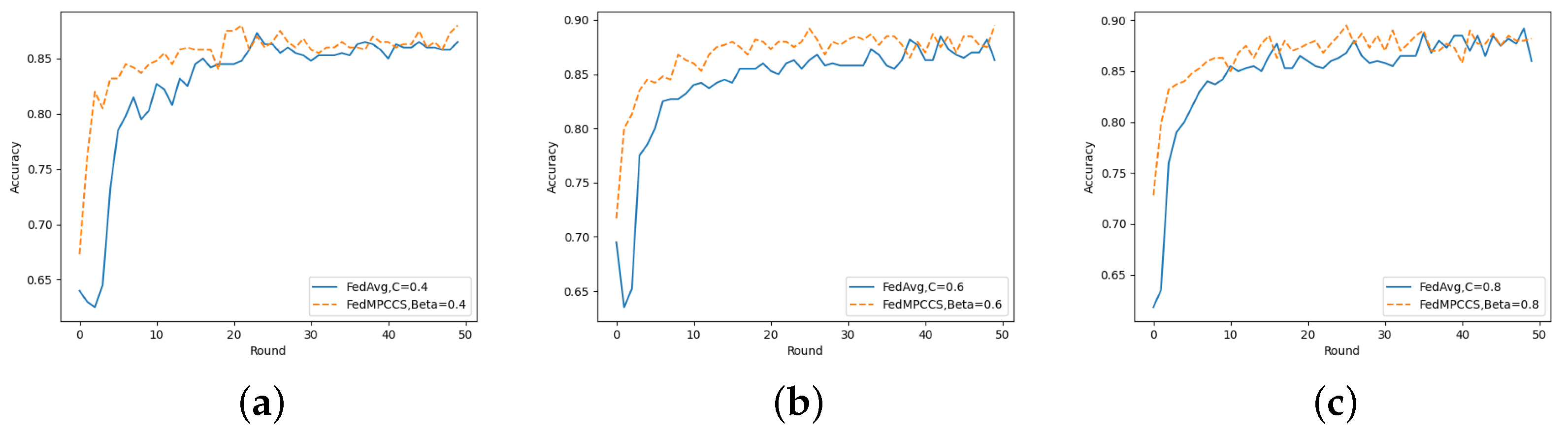
Figure 12 shows the variation in model accuracy for the same number of clients on the hard disk failure detection dataset for FedMPCCS and FedAvg. FedMPCCS in Figure 12a shows a faster accuracy improvement than FedAvg up to Round = 20, and the accuracy improvement of both algorithms plateaus after Round = 20. In Figure 12b, FedMPCCS has a significantly higher accuracy than FedAvg up to Round = 40. FedMPCCS in Figure 12c outperforms FedAvg for the vast majority of global communication rounds.

To compare the magnitude of the improvement in FedMPCCS with FedAvg on the two datasets, we counted and compared the average improvement in global communication rounds in accuracy of FedMPCCS over FedAvg, and the results are shown in

Table 2. Global average improvements in the accuracy of FedMPCCS over FedAvg on two different datasets.

Dataset	$\mathit{C},\mathit{\beta }=0.4$	$\mathit{C},\mathit{\beta }=0.6$	$\mathit{C},\mathit{\beta }=0.8$
Power system attack	1.74%	1.01%	0.93%
Hard drive failure detection	2.50%	2.65%	1.90%

:

6. Conclusions

Federated learning for smart manufacturing often suffers from data heterogeneity factors, and these problems seriously affect the effectiveness and accuracy of federated learning algorithms. This paper innovatively proposes a participant selection algorithm based on the variation in model parameters, applying similarity calculations and graph theory to calculate the multi-party similarity between clients to accurately measure the similarity between participants. By pre-selecting the initial set of participants, the data differences between devices can be effectively reduced and the federated learning training efficiency can be improved. Experimental results show that manufacturing data heterogeneity negatively affects the federated learning algorithm, the average accuracy of the comparison is reduced by up to 6.12% with IID data, and the approach described in this paper outperforms the baseline approach in terms of convergence and accuracy improvements, with a global average improvement in accuracy between 0.93% and 2.65% for different data and different parameter settings, reducing the impact of the heterogeneity factor. Future work will investigate composite methods for collecting client resource communication states combined with similarity calculations, which are geared towards more complex manufacturing federated learning application scenarios.

References

1. Khorasani, M.; Gibson, I.; Ghasemi, A.H.; Hadavi, E.; Rolfe, B. Laser subtractive and laser powder bed fusion of metals: Review of process and production features. Rapid Prototyp. J. 2023, 29, 935–958. [Google Scholar] [CrossRef]
2. Zheng, P.; Wang, H.; Sang, Z.; Zhong, R.Y.; Liu, Y.; Liu, C.; Mubarok, K.; Yu, S.; Xu, X. Smart manufacturing systems for Industry 4.0: Conceptual framework, scenarios, and future perspectives. Front. Mech. Eng. 2018, 13, 137–150. [Google Scholar] [CrossRef]
3. Wuest, T.; Weimer, D.; Irgens, C.; Thoben, K.D. Machine learning in manufacturing: Advantages, challenges, and applications. Prod. Manuf. Res. 2016, 4, 23–45. [Google Scholar] [CrossRef] [Green Version]
4. Wang, J.; Ma, Y.; Zhang, L.; Gao, R.X.; Wu, D. Deep learning for smart manufacturing: Methods and applications. J. Manuf. Syst. 2018, 48, 144–156. [Google Scholar] [CrossRef]
5. Kusiak, A. Smart manufacturing. Int. J. Prod. Res. 2018, 56, 508–517. [Google Scholar] [CrossRef]
6. Kapp, V.; May, M.C.; Lanza, G.; Wuest, T. Pattern recognition in multivariate time series: Towards an automated event detection method for smart manufacturing systems. J. Manuf. Mater. Process. 2020, 4, 88. [Google Scholar] [CrossRef]
7. Chai, Z.; Ali, A.; Zawad, S.; Truex, S.; Anwar, A.; Baracaldo, N.; Zhou, Y.; Ludwig, H.; Yan, F.; Cheng, Y. Tifl: A tier-based federated learning system. In Proceedings of the 29th International Symposium on High-Performance Parallel and Distributed Computing, Stockholm, Sweden, 23–26 June 2020; pp. 125–136. [Google Scholar]
8. Nguyen, D.C.; Ding, M.; Pathirana, P.N.; Seneviratne, A.; Li, J.; Poor, H.V. Federated learning for internet of things: A comprehensive survey. IEEE Commun. Surv. Tutor. 2021, 23, 1622–1658. [Google Scholar] [CrossRef]
9. Kairouz, P.; McMahan, H.B.; Avent, B.; Bellet, A.; Bennis, M.; Bhagoji, A.N.; Bonawitz, K.; Charles, Z.; Cormode, G.; Cummings, R.; et al. Advances and open problems in federated learning. Found. Trends Mach. Learn. 2021, 14, 1–210. [Google Scholar] [CrossRef]
10. McMahan, B.; Moore, E.; Ramage, D.; Hampson, S.; y Arcas, B.A. Communication-efficient learning of deep networks from decentralized data. In Proceedings of the 20th International Conference on Artificial Intelligence and Statistics, Fort Lauderdale, FL, USA, 20–22 April 2017; pp. 1273–1282. [Google Scholar]
11. Li, T.; Sahu, A.K.; Zaheer, M.; Sanjabi, M.; Talwalkar, A.; Smith, V. Federated optimization in heterogeneous networks. Proc. Mach. Learn. Syst. 2020, 2, 429–450. [Google Scholar]
12. Nishio, T.; Yonetani, R. Client selection for federated learning with heterogeneous resources in mobile edge. In Proceedings of the ICC 2019—2019 IEEE International Conference on Communications (ICC), Shanghai, China, 20–24 May 2019; pp. 1–7. [Google Scholar]
13. Palihawadana, C.; Wiratunga, N.; Wijekoon, A.; Kalutarage, H. FedSim: Similarity guided model aggregation for Federated Learning. Neurocomputing 2022, 483, 432–445. [Google Scholar] [CrossRef]
14. Wang, T.; Liu, Y.; Zheng, X.; Dai, H.N.; Jia, W.; Xie, M. Edge-based communication optimization for distributed federated learning. IEEE Trans. Netw. Sci. Eng. 2021, 9, 2015–2024. [Google Scholar] [CrossRef]
15. Karimireddy, S.P.; Kale, S.; Mohri, M.; Reddi, S.; Stich, S.; Suresh, A.T. Scaffold: Stochastic controlled averaging for federated learning. In Proceedings of the International Conference on Machine Learning, PMLR, Virtual, 13–18 July 2020; pp. 5132–5143. [Google Scholar]
16. Hink, R.C.B.; Beaver, J.M.; Buckner, M.A.; Morris, T.; Adhikari, U.; Pan, S. Machine learning for power system disturbance and cyber-attack discrimination. In Proceedings of the 2014 7th International Symposium on Resilient Control Systems (ISRCS), Denver, CO, USA, 19–21 August 2014; pp. 1–8. [Google Scholar]
17. Shen, J.; Wan, J.; Lim, S.J.; Yu, L. Random-forest-based failure prediction for hard disk drives. Int. J. Distrib. Sens. Netw. 2018, 14, 1550147718806480. [Google Scholar] [CrossRef]
Figure 1. Federated learning framework.
Electronics 12 02532 g001
Figure 2. Distribution of client-side data heterogeneity in federated learning.
Electronics 12 02532 g002
Figure 3. Federated learning of update directions for global and client-side models on different structured data.
Electronics 12 02532 g003
Figure 4. Process of client selection methods based on model parameter changes.
Electronics 12 02532 g004
Figure 5. An intelligent power system framework for power system attack datasets.
Electronics 12 02532 g005
Figure 6. Data distribution of parameter α at different settings.
Electronics 12 02532 g006
Figure 7. Performance of FedAvg’s algorithms for different sampling methods (IID and non-IID) on power system attack datasets.
Electronics 12 02532 g007
Figure 8. Algorithmic performance of FedAvg using power system attack datasets in different non-IID.
Electronics 12 02532 g008
Figure 9. Changes in loss reduction for FedMPCCS and FedAvg on power system attack dataset. (a) C , β = 0.4 , (b) C , β = 0.6 , (c) C , β = 0.8 .
Electronics 12 02532 g009
Figure 10. Change in loss reduction for FedMPCCS and FedAvg on hard disk failure detection datasets. (a) C , β = 0.4 , (b) C , β = 0.6 , (c) C , β = 0.8 .
Electronics 12 02532 g010
Figure 11. Rising variability in accuracy of FedMPCCS and FedAvg on power system attack datasets. (a) C , β = 0.4 , (b) C , β = 0.6 , (c) C , β = 0.8 .
Electronics 12 02532 g011
Figure 12. Rising variation in the accuracy of FedMPCCS and FedAvg on hard disk failure detection datasets. (a) C , β = 0.4 , (b) C , β = 0.6 , (c) C , β = 0.8 .
Electronics 12 02532 g012