Study on Downhole Geomagnetic Suitability Problems Based on Improved Back Propagation Neural Network

Abstract

The analysis of geomagnetic suitability is the basis and premise of geomagnetic matching navigation and positioning. A geomagnetic suitability evaluation model using mixed sampling and an improved back propagation neural network (BPNN) based on the gray wolf optimization (GWO) algorithm by incorporating the dimension learning-based hunting (DLH) search strategy algorithm was proposed in this paper to accurately assess the geomagnetic suitability. Compared with the traditional geomagnetic suitability evaluation model, its generalization ability and accuracy were better improved. Firstly, the key indicators and matching labels used for geomagnetic suitability evaluation were analyzed, and an evaluation system was established. Then, a mixed sampling method based on the synthetic minority over-sampling technique (SMOTE) and Tomek Links was employed to extend the original dataset and construct a new dataset. Next, the dataset was divided into a training set and a test set, according to 7:3. The geomagnetic standard deviation, kurtosis coefficient, skewness coefficient, geomagnetic information entropy, geomagnetic roughness, variance of geomagnetic roughness, and correlation coefficient were used as input indicators and put into the DLH-GWO-BPNN model for model training with matching labels as output. Accuracy, recall, the ROC curve, and the AUC value were taken as evaluation indexes. Finally, PSO (Particle Swarm Optimization)-BPNN, WOA (Whale Optimization Algorithm)-BPNN, GA (Genetic Algorithm)-BPNN, and GWO-BPNN algorithms were selected as compared methods to verify the predictable ability of the DLH-GWO-BPNN. The accuracy ranking of the five models on the test set was as follows: PSO-BPNN (80.95 %) = WOA-BPNN (80.95%) < GA-BPNN (85.71%) = GWO-BPNN (85.71%) < DLH-GWO-BPNN (95.24%). The results indicate that the DLH-GWO-BPNN model can be used as a reliable method for underground geomagnetic suitability research, which can be applied to the research of geomagnetic matching navigation.

1. Introduction

Navigation has a long history of development and plays an indispensable role in human production and life. Traditional navigation systems such as satellite and inertial navigation can no longer meet the requirements of long-endurance and high-precision navigation development in applications [1]. Geomagnetic navigation uses the features of the geomagnetic field for navigation and positioning, which has the advantages of being passive, all-day, and all-weather [2,3,4,5]. Additionally, it has become a new method for combined positioning of indoor and underground engineering [6].

The accuracy of geomagnetic matching navigation positioning is related to a large extent to the suitability of the geomagnetic map [7]. The suitability of the geomagnetic map represents the corresponding relationship between geomagnetic features and geographical location. The suitability directly affects the accuracy of geomagnetic matching navigation and positioning [8,9]. The matching area with good suitability contains more abundant geomagnetic features and information [10,11]. The analysis of geomagnetic suitability is the basis and premise of geomagnetic matching navigation positioning [12]. Therefore, the study of geomagnetic suitability analysis is of great significance.

In the current literature, researchers mainly improve the geomagnetic suitability evaluation method by constructing comprehensive suitability feature parameters or introducing intelligent classification algorithms.

Chen Y.R. et al. [13] used the fractal dimension as the feature parameter of geomagnetic suitability to evaluate the suitability. The outcomes demonstrated that this method had the advantages of a small calculation, good anti-interference, and simple implementation. Wang X.L. et al. [14] compared the selection methods of matching area based on geomagnetic suitability feature parameters and based on the information entropy of geomagnetic suitability feature parameters. The latter was found to be more effective.

Zhao J.H. et al. [15] proposed a matching area division method for underwater geomagnetic navigation based on the geomagnetic symbiosis matrix. This method can respond to the changing features of the geomagnetic field in multiple directions. Zhu Z.L. et al. [16] studied the sensitivity of multi-attribute weight in geomagnetic suitability evaluation using the Weighted Product Model (WPM) method. This study obtained the order of sensitivity of geomagnetic suitability indicators, which had certain reference significance for setting the geomagnetic map suitability feature weights.

Huang Z.X. et al. [17] adopted statistical parameters such as entropy and roughness as geomagnetic feature parameters. The correlation analysis of the feature parameters was carried out based on the matching test, and then the performance analysis of the matching area was realized. Liu Y.X. et al. [18] presented a new approach to selecting geomagnetic matching areas by integrating multiple feature parameters. The proposed approach was proven to be feasible through the simulation test. Li D.W. et al. [19] proposed a method to construct a comprehensive evaluation value based on factor analysis and entropy methods for suitability evaluation. The matching algorithm was used to simulate the experiment. The experiment verified the high agreement between comprehensive evaluation value and matching probability.

Wang Z. et al. [20] defined the concept of credibility and analyzed the credibility between four commonly used geomagnetic feature parameters and matching probability. It was found that a single feature parameter cannot be used as an effective basis for geomagnetic suitability evaluation. Wang P. et al. [21] comprehensively considered four characteristic parameters of a geomagnetic map. The decision method containing maximum deviation and entropy was used to construct the comprehensive evaluation value. The experiment was carried out to prove that the comprehensive evaluation value can be used as a quantitative basis for geomagnetic suitability analysis. Wang L.H. et al. [22] proposed a fuzzy, vague set evaluation method with more information based on the fuzzy decision method. Based on this method, the comprehensive evaluation value was constructed, and the simulation experiment was carried out. It was found that the matching error of the region with a large comprehensive evaluation value was small. Zhu Z.L et al. [23] fused the five indicators and used entropy technology to modify the weight of each indicator obtained based on traditional fuzzy evaluation methods to obtain the comprehensive evaluation value. The traditional Mean Square Differences (MSD) and Mean Absolute Differences (MAD) matching algorithms were used for simulation experiments. It was found that the comprehensive evaluation value and the matching probability were highly consistent, and the comprehensive evaluation value can comprehensively evaluate the geomagnetic suitability.

Zhong Y. et al. [24] used five main feature parameters as fuzzy indicators for weighted analysis to obtain a comprehensive evaluation value. An experimental study was conducted on the basis of the non-tracking Kalman filter with geomagnetic anomalies and the anomaly grid data of some waters in the South China Sea. Experiments showed that the proposed method was reliable. Zhang H. et al. [25] established a comprehensive evaluation model combining Principal Component Analysis (PCA) and Analytic Hierarchy Process (AHP) algorithms, which was used to evaluate the suitability. He Y.J. et al. conducted a comprehensive geomagnetic suitability evaluation based on AHP, the information entropy method [26], and the gray correlation method [27], respectively. The correlative matching algorithm was used to test it, and it was found that the comprehensive evaluation value and the matching probability are highly consistent.

Related experts and scholars on geomagnetic suitability evaluation have done a lot of work and achieved fruitful results by constructing the comprehensive evaluation value. The index system of this research is relatively simple, and the workload is large and cumbersome. There are a few types of research on suitability evaluation using classification algorithms. Additionally, most of them adopt the BPNN algorithm or an optimized BPNN algorithm. Zhang K. et al. [28] suggested automatic recognition and division methods for background field matching/mismatch areas based on BPNN. On the basis of the BPNN algorithm, Wang C.Y. et al. [29] combined PCA and GA to gain improved methods to evaluate geomagnetic suitability and improve classification accuracy. Wang J.H. et al. [30] studied the suitability of downhole geomagnetism by using the BPNN algorithm based on contribution factors. The accuracy of training sets was 95%, and the accuracy of test sets was close to 73%. The intelligent classification algorithm for suitability evaluation can decrease the subjective impact. At the same time, more geomagnetic suitability feature indicators can be involved in the calculation, making the evaluation results more comprehensive and improving the efficiency of geomagnetic suitability evaluation. It will be the focus of future geomagnetic suitability research.

The GWO algorithm is a population intelligence algorithm that has the characteristics of simple operation, few parameters, and easy implementation. It is often used to optimize the BPNN algorithm and is applied in engineering practice. Bao W. et al. [31], based on the battery operation data of the electric vehicle cloud platform with a sampling period of 10 s, used the data to test the unoptimized BPNN, GWO-BPNN, and PSO-BPNN. The experimental results indicate that the GWO-BPNN has high accuracy in predicting the SOC of electric vehicle batteries. Jing W.Q. et al. [32] proposed an improved GWO-BPNN energy consumption prediction model, which was validated using actual operating data of an office building in Xi’an. The prediction results showed that the prediction accuracy of the improved GWO-BPNN model was much higher than that of traditional prediction models. Guo Cui et al. [33] used the gray wolf population algorithm to optimize the BPNN to establish a dynamic model of the accelerometer and simulate the input and output signals. The results show that, compared with the BPNN algorithm, the algorithm has improved its solution accuracy by 43.4% after optimization and improvement. However, due to its tendency to fall into local optima, the GWO algorithm needs to be improved to achieve a balance between local and global search. Li Z. et al. [34] proposed a binary version of the local adversarial learning golden sine gray wolf optimization algorithm and verified its high search accuracy. Pan H. et al. [35] proposed an improved gray wolf optimization algorithm for feature selection of high-dimensional data. Pan T et al. [36] integrated the nonlinear convergence factor and position mutation strategy into GWO to solve the problem of complex and non-linear components and prevent the gray wolf algorithm from falling into a local optimum.

Traditional suitability evaluation methods were mostly applied in the air and underwater. There was little research on downhole suitability evaluation methods. To select more suitable areas for matching, this paper constructs an intelligent model for geomagnetic suitability evaluation based on multi-algorithm coupling. Firstly, a mixed sampling method was constructed by combining SMOTE and Tomek Links to process the original datasets collected from 41 underground engineering projects and obtain a new dataset. Secondly, a hybrid optimization algorithm based on the DLH algorithm and the GWO algorithm is used to optimize the parameters of the BPNN algorithm, and the DLH-GWO-BPNN algorithm is used to construct a geomagnetic suitability model. Then, using accuracy, recall, AUC value, and ROC curve as evaluation indicators, PSO-BPNN, WOA-BPNN, GA-BPNN, and GWO-BPNN algorithms were selected as compared methods to verify the predictable ability of the DLH-GWO-BPNN. The results showed that this model can effectively evaluate geomagnetic suitability and has reference significance for intelligent geomagnetic navigation.

The remainder of this paper is organized as follows: The GWO algorithm and the BPNN algorithm are described in Section 2; the DLH-GWO-BPNN model is shown in Section 3; Section 4 shows the data processing results and the analysis results; and the conclusion is given in Section 5.

2. Related Work

2.1. GWO Algorithm

The gray wolf optimization (GWO) algorithm is an optimization method for swarm intelligence [37]. It simulates the leading status and relatively complete hunting process of gray wolves in their natural environment. Additionally, it is widely used because of its simple structure, few adjustable parameters, and strong convergence performance.

The algorithmic content is as follows:

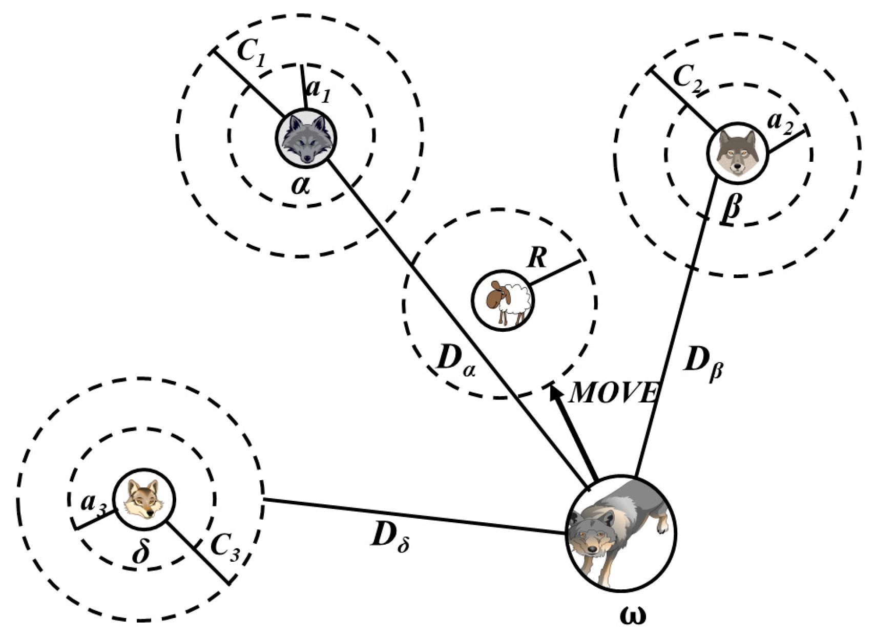
In GWO algorithm, there are four levels of wolves, as illustrated in Figure 1. α wolf is the head gray wolf. α wolf, as the leader, is in charge of all kinds of activities among the wolves and is the most capable of managing them. β wolf obeys the orders of α, can dominate other gray wolves, and is the best successor of the head gray wolf. δ wolf assists the decision-making of the β wolf and obeys the management of the α wolf and β wolf. The ω wolf is the last level of the social hierarchy, and its presence effectively prevents internal problems such as fighting each other.

The GWO algorithm includes five parts:

(1)

Social level

In GWO algorithm, there are four levels of gray wolf population: α, β, δ and ω. The rank of society is α, β, δ, and ω. The α, β, and δ are also the three gray wolves with the best fitness in each generation’s population, which are constantly updated in the iterative process of the GWO algorithm.

(2)

Surrounding prey

α, β, and δ directly capture prey. ω wolf surrounds prey. Its surrounding process is described by Formulas (1) and (2).

$$Q=\left|C\times Y_p(t)-Y(t)\right|$$

(1)

$$Y(t+1)=Y_p(t)-A\times Q$$

(2)

Formula (1) is the distance between any gray wolf in the gray wolf population and prey. Formula (2) is the updated formula for the offspring of the gray wolves. Y(t) and Y(t + 1) represent the positions of gray wolves after the tth iteration and the (t + 1)th iteration, respectively. Y_p(t) is the position of prey. A and C are the coefficients, which are obtained according to Formulas (3) and (4):

$$A=2a\times n_2-a$$

(3)

$$C=2n_1$$

(4)

a is a control factor, and it is linear. n₁ is a random number between 0 and 1. The value range of n₂ is within [0, 1].

(3)

Hunting

α, β, and δ are the best three wolves. They find the location of prey, notify ω, and round up the prey. The α, β, and δ determine the location of prey. ω, according to the positions of α, β, and δ, constantly adjusts its position. The mathematical principle is described by the following formula:

$$Q_{\alpha }=\left|C_1\times Y_{\alpha }(t)-Y(t)\right|$$

(5)

$$Q_{\beta }=\left|C_2\times Y_{\beta }(t)-Y(t)\right|$$

(6)

$$Q_{\delta }=\left|C_3\times Y_{\delta }(t)-Y(t)\right|$$

(7)

Q_α, Q_β, and Q_δ are the distances between α, β, and δ wolf and other individuals, respectively. Y_α(t), Y_β(t), and Y_δ(t) represent the positions of α, β, and δ after the tth iteration, respectively. C_i is an adaptive vector.

$$Y_1=Y_{\alpha }-A_1\times Q_{\alpha }$$

(8)

$$Y_2=Y_{\beta }-A_2\times Q_{\beta }$$

(9)

$$Y_3=Y_{\delta }-A_3\times Q_{\delta }$$

(10)

$$Y\left(t+1\right)=\frac{\left(Y_1+Y_2+Y_3\right)}{3}$$

(11)

Y₁, Y₂, and Y₃ represent the direction and distance of the ω wolf to the α wolf, β wolf, and δ wolf, respectively. Formula (11) is the final position of the wolf pack. A_i is a random vector.

According to the above formulas, gray wolves track and round up prey, as shown in Figure 2:

(4)

Attacking prey

When the prey is still in place, the whole wolf pack attacks. The process of attacking prey in GWO is simulated. It can be seen from Formula (3) that as a decreases, A also decreases continuously. In the iteration process, a decreases from 2 to 0, which is a linear change process, and A also changes in the corresponding interval. A controls the expansion and contraction of the encirclement circle of the gray wolf pack. When |A| > 1, the whole wolf pack will move far away from the prey in order to find optimal prey; that is global search. When |A| < 1, the whole wolf pack will move to the location of the prey and launch an attack; that is local search. The schematic diagram of this process is shown in Figure 3.

(5)

Searching prey

When |A| > 1, they will go away from the prey, then globally search for other better prey. Because of the randomness of the parameter C in finding prey, the algorithm has a stochastic search behavior. In the algorithm design, it has a certain avoidance effect on falling into the local optimum. It also acts as an obstacle in nature that prevents the wolf population from capturing prey easily.

2.2. BPNN Algorithm

BPNN algorithm has strong fault tolerance and generalization ability, which are applied in many fields [38]. The structure of BPNN has three sections, the configuration of which is illustrated schematically in Figure 4. The neurons in the input layer can obtain the dataset. The hidden layer is located in the middle of the input and output layers. The dataset of the input layer is transformed and processed by the hidden layer, and then sent to the output layer to obtain the final result.

The mathematical principles of BPNN are divided into the following two parts:

(1)

Forward propagation

Forward propagation means that the neural network calculates and stores the intermediate variables in sequence, from input layer to hidden layer and then to output layer. After the parameters of BPNN are initialized, the training data are input from the input layer and then transmitted to the hidden layer, and the input of the neurons in the hidden layer is obtained.

$$Z_j={\displaystyle \sum _{i=1}^n{v}_{ij}{x}_j}\begin{array}{cc}& j=1,2,\dots ,q\end{array}$$

(12)

Z_j represents the input value of the jth neuron of the hidden layer. X_i represents the input value of the ith neuron of the input layer, namely the sample data. v_ij represents the connection weight.

The output values of neurons in the hidden layer are calculated according to the thresholds and the input values of the neurons in the hidden layer. The calculation formula for the output value is:

$$M_j=f_1(Z_j-a_j)\begin{array}{cc}& j=1,2,\dots ,q\end{array}$$

(13)

f₁ represents the transfer function. a_j is the threshold of the jth neuron in the hidden layer. M_j is the output value of the jth neuron in the hidden layer.

According to the output value M_j of the hidden layer and the given weights, calculate the results and transfer them to the output layer as input values. The input of the output layer is obtained.

$$O_k={\displaystyle \sum _{j=1}^q{w}_{jk}{M}_j}\begin{array}{cc}& k=1,2,\dots ,m\end{array}$$

(14)

O_k represents the input value of the kth neuron in the output layer. w_jk represents the weight.

According to the thresholds of neurons in the output layer and the input value of the output layer, the output value of the neurons in the output layer is calculated and obtained. The calculation formula for the output value is:

$$N_k=f_2(O_k-b_k)\begin{array}{cc}& k=1,2,\dots ,m\end{array}$$

(15)

N_k is the output value of the kth neuron in the output layer. f₂ is the transfer function. b_k is the threshold of the kth neuron in the output layer.

(2)

Back propagation

Back propagation refers to the calculation method of BPNN parameter gradient. According to the chain rule of calculus, the gradient of loss function for each parameter in the BPNN algorithm is calculated in sequence from the output to the input, and the parameters are updated with the optimization method to reduce the loss function.

According to N_k and Y_k of each neuron, the error of BPNN is obtained.

$$E=\frac{1}{2}{\displaystyle {\sum }_{k=1}^m(Y_k-N_k)}$$

(16)

E is the error in BPNN. Y_k is the expected output value. N_k is the actual output value.

When the error is not within the acceptable range, v_ij, w_jk, a_j, and b_k are adjusted according to the gradient descent theory and chain rule. The correction values of v_ij, w_jk, a_j, and b_k are obtained.

$$\Delta v_{\mathit{ij}}=-\eta \frac{\partial E}{\partial v_{ij}}=-\eta (\frac{\partial E}{\partial M_j})(\frac{\partial M_j}{\partial v_{ij}})=-\eta (\frac{\partial E}{\partial M_j})(\frac{\partial M_j}{\partial Z_j})(\frac{\partial Z_j}{\partial v_{ij}})$$

(17)

$$\Delta v_{jk}=-\eta \frac{\partial E}{\partial w_{jk}}=-\eta (\frac{\partial E}{\partial N_k})(\frac{\partial N_k}{\partial w_{jk}})=-\eta (\frac{\partial E}{\partial N_k})(\frac{\partial N_k}{\partial O_k})(\frac{\partial O_k}{\partial w_{jk}})$$

(18)

$$\Delta a_j=-\eta \frac{\partial E}{\partial a_j}=-\eta (\frac{\partial E}{\partial M_j})(\frac{\partial M_j}{\partial a_j})$$

(19)

$$\Delta b_k=-\eta \frac{\partial E}{\partial b_k}=-\eta (\frac{\partial E}{\partial N_k})(\frac{\partial N_k}{\partial b_k})$$

(20)

η indicates learning rate. The value range of η is within [0, 1].

The revised weights and thresholds are:

$$\begin{array}{l}{v}_{\mathit{ij}}=v_{\mathit{ij}}+\Delta v_{\mathit{ij}}\\ w_{\mathit{jk}}=w_{\mathit{jk}}+\Delta w_{\mathit{jk}}\\ a_j=a_j+\Delta a_j\\ b_k=b_k+\Delta b_k\end{array}$$

(21)

After the weights and thresholds are updated, forward propagation is carried out to make the actual output approximate the theoretical output to the greatest extent.

2.3. The SMOTE and Tomek Links Method

(1)

SMOTE

Synthetic Minority Oversampling Technique (SMOTE) is a classic oversampling method to deal with data imbalance. A synthetic sample is generated by taking the corresponding line segment of two minority samples as the endpoints to increase the number of minority samples and achieve the purpose of oversampling minority samples. The principle of SMOTE in making the new sample is shown in Formula (22).

$$x_{new}=x+rand(0,1)\times \left|\left|\stackrel{\wedge }{x}-x\right|\right|$$

(22)

x_new represents a new sample; x is a minority sample; $\stackrel{\wedge }{x}$ means the nearest neighbor sample.

(2)

Tomek Links

After oversampling, if the last two samples belong to two categories, the two samples are combined into a Tomek Links pair. One of the samples is noise data, and this sample is deleted. Tomek Links can effectively delete the overlapping data, which enables the classifier to classify better.

2.4. Evaluation Indicators of Model Performance

(1)

Accuracy

For a given set of samples, the calculation formula for accuracy is defined as follows:

$$A\mathit{ccuracy}=\frac{TP+TN}{TP+TN+FP+FN}$$

(23)

TP represents positive samples predicted by the model as positive classes; TN represents negative samples predicted by the model as negative classes; FP represents negative samples predicted by the model as positive; FN represents positive samples predicted by the model as negative classes.

(2)

Recall

The calculation formula for recall is shown in Equation (24).

$$\mathit{Recall}=\frac{TP}{TP+FN}$$

(24)

(3)

ROC curve and AUC

ROC (Regional Operating Characteristic) curve and AUC (Area Under Curve) are indicators for the comprehensive evaluation of binary classification problem. ROC curve provides a new graphical measurement of algorithm performance. The curve, which is close to the upper left corner, indicates the corresponding algorithm has good performance. AUC is the area under the ROC curve, and its value is within [0, 1]. The value that is close to 1 indicates an excellent result. This value can quantify the performance of the classification algorithm. In this paper, the idea of the ROC curve applied to multi-class classification is to plot the average ROC curve. Convert the sample label to a binary-like form, and then calculate the probability value of each sample under each label, and the average ROC curve is obtained.

3. DLH-GWO-BPNN Model

The GWO algorithm based on DLH is applied to optimize BPNN and construct the DLH-GWO-BPNN model.

3.1. Improved GWO Algorithm Based on DLH

The candidate positions in the GWO algorithm are mainly determined by α, β, and δ, which easily fall into the local optimal solution. To keep the balance between local and global search, the DLH algorithm is introduced to optimize the GWO algorithm. The inspiration for DLH comes from the hunting behavior of individuals in nature [39]. In the GWO algorithm, the concept of neighborhood is introduced to provide a new choice of candidate location for every gray wolf. The improved GWO algorithm based on DLH consists of three stages: the initialization phase, the movement phase, and the selection and update phases.

(1)

Initialization

According to Formula (25), determine the scope of the search space, in which N gray wolves are randomly initialized.

$$Y_{\mathit{km}}=L_k+ran{d}_m[0,1]\times \left(u_k-l_m\right) k\in [1,N],m\in [1,D]$$

(25)

Y_k(t) = {y_k1, y_k2, …y_kD} denotes the position of the kth gray wolf after the tth iteration. D is the dimension of the problem. The fitness function is f(x). Calculate Y_k(t) fitness according to f(x).

(2)

Movement

Individual hunting is not only an important behavior in the whole gray wolf population but also the inspiration for improving the GWO algorithm. In the DLH algorithm, every gray wolf is considered by their neighbors to be a candidate position after the tth iteration. The conventional GWO algorithm and the DLH algorithm generate new candidate positions as follows:

GWO: On the basis of the positions of α wolf, β wolf, and δ wolf and the calculated coefficients a, A, and C, determine the encirclement of the wolves. Then calculate the new candidate position Y_k-GWO(t + 1) after the tth iteration of the kth gray wolf according to Formula (11).

DLH: Each gray wolf learns from its neighbors and other random individuals, resulting in the new candidate position Y_k-DLH(t + 1) in the following steps.

Step 1: Calculate the euclidean distance between the current position and the candidate position Y_k-GWO(t + 1) of each gray wolf of the GWO algorithm. According to this distance, calculate the search radius R_k(t) of every gray wolf.

$$R_k\left(t\right)=\sqrt{{[Y_k(t)-Y_{k\text{-}GWO}(t+1)]}^2}$$

(26)

Step 2: Determine the neighborhood of Y_k(t) with the following expression.

$$N_k(t)=\left\{\left.Y_m(t)\right|Q_k(Y_k(t),Y_m(t))\le R_k(t),Y_m(t)\in Pop\right\}$$

(27)

Q_k denotes the Euclidean distance between Y_k(t) and Y_m(t). Pop represents a matrix that stores wolves. It has N rows and D columns.

Step 3: Select randomly the neighborhood Y_n,d(t) in N_k(t). Select randomly Y_r,d(_t) from Pop. The new candidate position Y_k-DLH(t + 1) is calculated according to these two quantities.

$$Y_{k\text{-}DLH,d}(t+1)=Y_{k,d}(t)+rand\times (Y_{n,d}(t)-Y_{r,d}(t))$$

(28)

(3)

Selection and updating

The excellent candidate position is selected by calculating and comparing the fitness of the two positions with the following mathematical expression.

$$Y_k(t+1)=\left\{\begin{array}{ll}{Y}_{k\text{-}GWO}(t+1)\hfill & if\hspace{1em}f(Y_{k\text{-}GWO})<f(Y_{k\text{-}DLH})\hfill \\ Y_{k\text{-}DLH}(t+1)\hfill & Otherwise\hfill \end{array}\right.$$

(29)

Based on this principle, update the position of each gray wolf until it reaches the largest number of iterations.

3.2. DLH-GWO-BPNN Model

In the evaluation of geomagnetic suitability, in order to improve the accuracy of the traditional BPNN model, the collected test data are mixed-sampled. After data preparation, the DLH-GWO algorithm is used to optimize the traditional BPNN model and build the DLH-GWO-BPNN model.

The specific steps are as follows:

Step 1: Construction of a mixed sampling method based on the SMOTE and Tomek Links algorithms. The SMOTE algorithm is used to synthesize the unmatched samples, weakly matched samples, and matched samples in the original dataset. Use the Tomek Links algorithm for data cleaning. Then normalize the sampled dataset.

Step 2: Set the maximum number of iterations of the DLH-GWO algorithm. Determine the topology of BPNN.

Step 3: The initial dimension represents the initial weight and threshold of BPNN. Put it into BPNN for training. Calculate the fitness of each gray wolf in the wolf pack. Select the three gray wolves with the lowest fitness value. Ranked from small to large according to fitness, namely α, β, and δ.

Step 4: Update the position of each gray wolf according to Formulas (8)–(11), namely Y_k-GWO(t + 1). Then construct a new neural network for training. Recalculate the fitness of each gray wolf. Select the three gray wolves with the lowest fitness value. Ranked from small to large according to fitness, namely α, β, and δ. Update the position of each gray wolf again, namely Y_k-GWO(t + 1).

Step 5: Calculate the search radius of each gray wolf according to Formula (26). Then determine the neighborhood of each gray wolf according to Formula (27). Each time a gray wolf learns from its neighbors and other random individuals, a new candidate position is generated, namely Y_k-DLH(t + 1).

Step 6: Calculate the fitness of Y_k-GWO(t + 1) and Y_k-DLH(t + 1). Compare and select excellent candidates for the position.

Step 7: Judge whether the maximum number of iterations of DLH-GWO has been reached. If not, return to Step 3. If so, record α corresponding initial weights and thresholds.

Step 8: Obtain the value range of the number of hidden layer nodes based on empirical formulas. Input the optimal initial weight and threshold into the BPNN for training. Set different numbers of nodes and activation functions for experiments. Carry out a comparative analysis and select the node number and activation function with the smallest error.

Step 9: Take the accuracy, recall, ROC curve, and AUC value as evaluation indicators and put the test set into the trained BPNN for validation analysis.

Traditional geomagnetic suitability evaluation models are mostly based on multiple geomagnetic features to build a comprehensive evaluation value. Then, through simulation experiments, verify the high consistency of the comprehensive evaluation value and the matching probability. Due to the numerous geomagnetic features, the selection of geomagnetic features for the construction of comprehensive evaluation values has greater subjectivity. In order to improve this situation, the data from the matching region is divided into four types of samples with different matching degrees according to the matching probability. The BPNN algorithm is introduced, and the geomagnetic features are taken as input and the matching labels are taken as output to evaluate suitability.

Because the BPNN algorithm is easy to overfit and excessively depends on the initial weight and threshold, the GWO algorithm is introduced to iteratively optimize the initial weight and threshold of the BPNN. The DLH algorithm is introduced to avoid the GWO algorithm falling into a local optimal solution. In addition, due to the imbalance of the proportion of each category of sample data selected, before training, a mixed sampling method is built based on the SMOTE and Tomek Links algorithms for data balance processing. Figure 5 describes the overall concept of the model.

4. Experimental Simulation

4.1. Selection of Indicators

According to the existing research, there are various feature parameters to characterize geomagnetic maps, such as geomagnetic roughness, geomagnetic standard deviation, geomagnetic information entropy, etc. The features of a geomagnetic map are characterized from different angles. Due to the incompleteness of a single feature to characterize geomagnetic suitability, seven indicators are selected from three aspects in combination with the distribution characteristics of the downhole geomagnetic field: macroscopic features, microscopic features, and self-similar features, and the geomagnetic suitability is comprehensively measured. The feature parameters are defined as follows:

The span of latitude and longitude of a candidate geomagnetic field area is set as the B × L grid, and g(k, m) is the geomagnetic strength value at the grid point coordinate (k, m).

4.1.1. Macroscopic Features

(1)

Geomagnetic standard deviation σ

σ is the reflection of the degree of dispersion of geomagnetic data and the general changes of the geomagnetic area in the candidate region. The large σ corresponds to the area with the apparent variation of geomagnetic features, and it is beneficial for the analysis of geomagnetic suitability. It is defined as follows:

$$\sigma =\sqrt{\frac{1}{BL-1}}{{\displaystyle \sum _{k=1}^B{\displaystyle \sum _{m=1}^L\left(g\left(k,m\right)-\overline{g}\right)}}}^2$$

(30)

$\overline{g}$ is the average geomagnetic field value, which is defined as follows:

$$\overline{g}=\frac{1}{BL}{\displaystyle \sum _{k=1}^B{\displaystyle \sum _{m=1}^{L}g(k,m)}}$$

(31)

(2)

Kurtosis coefficient C₁

C₁ stands for the concentration degree of geomagnetic field data in the candidate region. The larger the C₁, the more data are concentrated near the average geomagnetic field value, which is not conducive to matching. It is defined as:

$$C_1=\frac{1}{BL}{{\displaystyle \sum _{k=1}^B{\displaystyle \sum _{m=1}^L\frac{\left(g\left(k,m\right)-\overline{g}\right)}{{\sigma }^4}}}}^4-3$$

(32)

(3)

Skewness coefficient C₂

C₂ represents the symmetry of the geomagnetic map and is proportional to the suitability, which is defined as:

$$C_2=\frac{1}{BL}{{\displaystyle \sum _{k=1}^B{\displaystyle \sum _{m=1}^L\frac{\left(g\left(k,m\right)-\overline{g}\right)}{{\sigma }^3}}}}^3-3$$

(33)

4.1.2. Microscopic Features

(1)

Geomagnetic information entropy H

H reflects the fluctuation features of the geomagnetic field data and the richness of geomagnetic information in the candidate region. The lower the H, the better the matching effect. It is defined as:

$$\begin{array}{l}H=-{\displaystyle \sum _{k=1}^B{\displaystyle \sum _{m=1}^{L}p(k,m)}}lb\left[p(k,m)\right]\\ p(k,m)=\frac{\left|g(k,m)\right|}{{\displaystyle \sum _{k=1}^B{\displaystyle \sum _{m=1}^L\left|g(k,m)\right|}}}\end{array}$$

(34)

(2)

Geomagnetic roughness r

r reflects the local fluctuation state and average smoothness of the geomagnetic field in a candidate region. The greater the geomagnetic roughness, the more abundant the geomagnetic field information in the candidate region. It is defined as:

$$\begin{array}{l}r=\frac{r_x+r_y}{2}\\ r_x=\sqrt{\frac{1}{B(L-1)}{\displaystyle \sum _{k=1}^B{\displaystyle \sum _{m=1}^{L-1}{\left[g(k,m)-g(k,m+1)\right]}^2}}}\\ r_y=\sqrt{\frac{1}{L(B-1)}{\displaystyle \sum _{k=1}^{B+1}{\displaystyle \sum _{m=1}^L{\left[g(k,m)-g(k,m+1)\right]}^2}}}\end{array}$$

(35)

(3)

Variance of geomagnetic roughness R

R indicates the local fluctuation of geomagnetic data in the candidate region. The more significant the R, the more conducive the analysis of geomagnetic suitability is. It is defined as:

$$R=\frac{r}{\sigma }$$

(36)

4.1.3. Self-Similar Features

(1)

Correlation coefficient p

The p reflects the independence of geomagnetic field values in the candidate region. A small correlation coefficient corresponds to good matching performance. It is defined as:

$$\begin{array}{l}p=\left(p_x+p_y\right)\\ p_x=\frac{1}{B(L-1){\sigma }^2}{\displaystyle \sum _{k=1}^B{\displaystyle \sum _{m=1}^{L-1}\left[g(k,m)-\overline{g}\right]}}\left[g(k,m+1)-\overline{g}\right]\\ p_y=\frac{1}{L(B-1){\sigma }^2}{\displaystyle \sum _{k=1}^{B-1}{\displaystyle \sum _{m=1}^L\left[g(k,m)-\overline{g}\right]}}\left[g(k+1,m)-\overline{g}\right]\end{array}$$

(37)

4.2. Matching Labels

Calculate the matching probability of the selected sample area according to the matching algorithm. According to the matching probability, samples are divided into four kinds of matching labels: 0 (mismatch), 1 (weak match), 2 (match), and 3 (strong match), as shown in

Table 1. Matching labels.

Matching Probability	Matching Labels
p ≤ 0.45	0 (mismatch)
0.45 < p < 0.65	1 (weak match)
0.65 < p < 0.85	2 (match)
p ≥ 0.85	3 (strong match)

[30].

4.3. Data Source and Data Processing

The model is trained with geomagnetic feature data and matching labels. The data are the geomagnetic features dataset collected by 41 underground projects of about 3 m, which is derived from the relevant data published in the related literature [30].

The data are processed as follows:

(1)

Mixed sampling

The original data contains five unmatched samples, six weakly matched samples, ten matched samples, and twenty strongly matched samples. This dataset is unbalanced and has a small amount of data. To improve the accuracy of the model, balance the data. SMOTE is used for oversampling the other three types of small samples except for strongly matched samples, and then the Tomek Links algorithm is used to delete overlapping samples between classes.

Finally, 68 samples were obtained, and

Table 2. Dataset after mixed sampling.

Serial Number	$\mathit{\sigma }$	C1	C2	H	r	R	p	Labels
1	11,818	1.6881	−2.5622	16,473	1.3939	6.3047	0.0179	3
2	6964.541	0.349015	−2.5202	4521.212	0.647512	6.38597	0.759121	1
3	4250.2	0.0838	−3.5289	3712.8	0.8736	6.6215	0.5636	3
4	14,625	6.0878	−0.9359	21,369	1.4612	5.9963	−0.1002	3
5	6414.256	0.482088	−2.72181	4106.584	0.638222	6.561462	0.762074	1
…	…	…	…	……	…	…	…	…
16	11,286.07	−0.57358	−2.58439	7393.175	0.660016	6.018778	0.72169	2
17	10,789	10.3652	−0.8811	12,113	1.1228	6.5529	0.2212	0
18	16,590	−0.0284	−2.2259	8129	0.49	6.0914	0.8545	2
19	14,220.52	3.797962	−1.34783	15,780.6	1.11081	6.572354	0.396289	2
20	650.5	6.8366	−4.9311	708.24	1.0888	6.4428	0.3211	3
…	…	…	…	…	…	…	…	…
29	2216.8	7.8613	−0.4768	2469.9	1.1142	6.8691	0.3056	0
30	9087.2	−0.6742	−2.6388	6393.1	0.7035	5.9621	0.6541	3
31	2320.041	7.832956	−0.47323	2440.805	1.122647	6.841694	0.303817	0
32	11,340.89	2.712972	−2.2966	14,995.35	1.320588	6.081461	0.087038	2
33	1806	2.9841	−1.6298	1785.98	0.9889	6.2846	0.4735	1
…	…	…	…	…	…	…	…	…
42	7508.8	0.2174	−2.3208	4931.3	0.6567	6.2124	0.7562	1
43	10,605.21	1.192791	−2.72845	12,728.04	1.203763	6.013634	0.199467	2
44	2391.321	7.815665	−0.48272	2530.774	1.1249	6.837674	0.302056	0
45	13,298	5.5214	−1.1896	17,868	1.3436	6.2463	0.0653	2
46	24,494	5.89	−0.8636	32,567	1.3296	6.567	0.014	2
47	24,494	5.89	−0.8636	32,567	1.3296	6.567	0.014	2
…	…	…	…	…	…	…	…	…
54	2274.525	7.845452	−0.47481	2453.632	1.118923	6.853777	0.304603	0
55	9720.771	4.248036	−1.53844	9295.326	0.940299	6.120685	0.50231	1
56	2326.8	7.8311	−0.473	2438.9	1.1232	6.8399	0.3037	0
57	2296.22	7.839496	−0.47406	2447.518	1.120698	6.848018	0.304228	0
63	11,248	0.3364	−2.6439	12,366	1.0994	5.7203	0.2995	3
…	…	…	…	…	…	…	…	…
65	2216.8	7.8613	−0.4768	2469.9	1.1142	6.8691	0.3056	0
66	6967.4	4.9571	−1.4596	6196.5	0.8894	5.9601	0.5265	1
67	19,384	1.9381	−1.7755	24,894	1.2842	6.5517	0.1174	3
68	2216.8	7.8613	−0.4768	2469.9	1.1142	6.8691	0.3056	0

shows part of the samples.

(2)

Normalization

The dataset is normalized to eliminate the impact of dimension.

$$y=\frac{(Ma{x}_y-Mi{n}_y)(x-Mi{n}_x)}{Ma{x}_x-Mi{n}_x}+Mi{n}_y$$

(38)

4.4. Parameter Selection of BPNN

(1)

Selection of neuron numbers

The number range of neurons in the hidden layer of BPNN is determined according to the empirical Formula (39).

$$m=\sqrt{n+l}+a$$

(39)

m, n, and l represent the number of neurons in the input, hidden, and output layers, respectively. a is an integer within [1,10].

The value within the range is selected as the number of neurons in the hidden layer, respectively. The average accuracy of the training set and test set is obtained through 70 tests to choose the optimal number.

(2)

Selection of the activation function of BPNN

Activation functions are set in the input-hidden layer and hidden-output layer, respectively. The softmax function is suitable for multi-classification neural network output, so the softmax function is selected as the activation function in the hidden-output layer. Carry out ten experiments and take the tansig, softmax, purelin, and radbas functions as activation functions in the input-hidden layer, respectively, then calculate and compare the average accuracy of the training and test sets under the training of the BPNN algorithm.

• tangsig function

$$\tan sig(x)=\frac{2}{1+e^{-2x}}-1$$

(40)

2.

softmax function

$$\sigma (X_i)=\frac{\exp (x_i)}{{\displaystyle \sum _{j=1}^n\exp (x_j)}}$$

(41)

3.

purelin function

$$y=x$$

(42)

4.

radbas function

$$y=\exp (-x^2)$$

(43)

4.5. Experimental Comparison

To verify the predictability of the proposed algorithm, comparative experiments were conducted. The BPNN is optimized by using five different optimization algorithms, namely WOA, GA, PSO, GWO, and DLH-GWO, and the model is constructed. Train the model with geomagnetic features as input and matching labels as output. By adjusting the main hyperparameter of each model, the optimal parameters of each model are obtained, respectively, and then the optimal model is constructed. Place the test set into the optimal model obtained, with geomagnetic features as input and matching labels as output. Evaluate the effect of each model using accuracy, recall, AUC value, and ROC curve as indicators.

5. Results and Analysis

5.1. Selection of Neuron Numbers

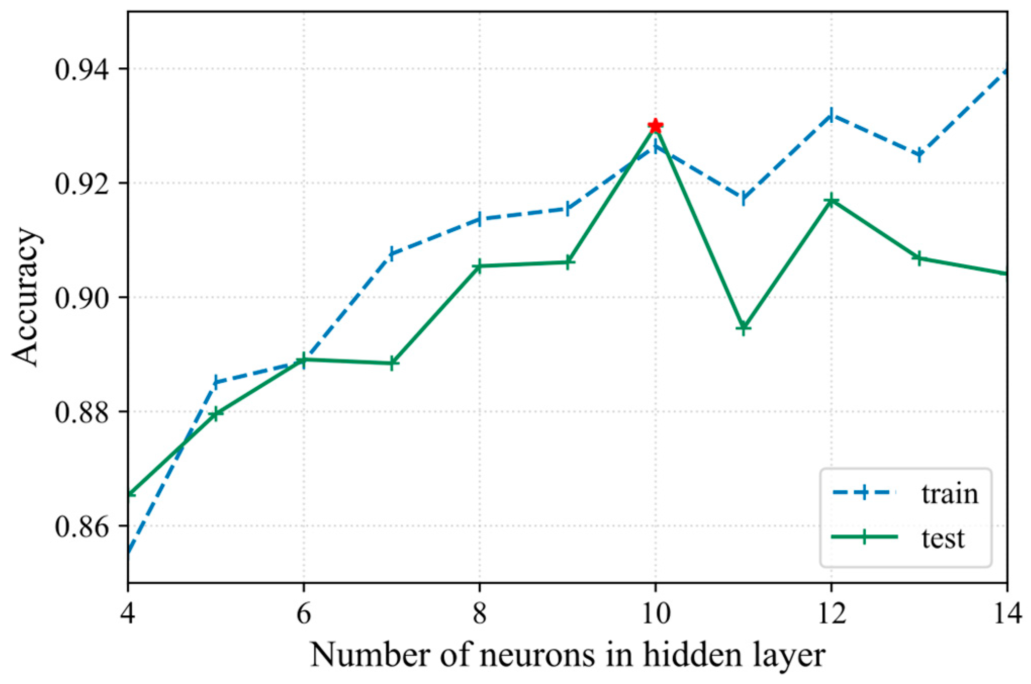
According to the empirical Formula (39), the number range of neurons in the hidden layer is within [4,14]. Different numbers of neurons are set, respectively, and experiments are conducted to obtain the corresponding average accuracy. The results are shown in Figure 6.

According to Figure 6, when the number of neurons is 10, the average accuracy in the test set reaches its highest, at 0.9299. Meanwhile, the average accuracy of the training set at this point is relatively high, at 0.9264. When the number of neurons is 12 or 14, the average accuracy in the training set is higher than that when the number of neurons is 10, but the average accuracy of the test set at these two points is lower in comparison. The average accuracy in the test set no longer increases more than that of the number of neurons, which is 10. Thus, the optimal number of neurons is 10.

5.2. Selection of Activation Function

The softmax function is suitable for multi-classification neural network output, so the softmax function is set as the activation function between the hidden layer and the output layer. Take tansig, softmax, purelin, and radbas functions as activation functions between the input layer and the hidden layer, respectively. Carry out 10 experiments and calculate and compare the average accuracy of the DLH-GWO-BPNN model in the training set and test set. The results are shown in

Table 3. Input-hidden layer activation function and average accuracy.

Activation Function	Accuracy of the Training Set (%)	Accuracy of the Test Set (%)
tansig	94.26	92.38
radbas	93.83	89.05
softmax	83.40	88.10
purelin	87.45	86.67

.

Using tansig, softmax, purelin, and radbas functions between the input layer and the hidden layer, respectively, the accuracy of the training set and the test set is different. When the purelin function or softmax function is used, the average accuracy of the test set and training set is below 90%. The softmax function has a good advantage for the output of the multi-classification neural network, but it is not ideal when used as the activation function in the input-hidden layer. When the radbas function is used, the average accuracy of the training set reaches 93.83%, but the average accuracy of the test set is relatively low. When the tansig function is used, the average accuracy of the test set and training set is above 90%, and identification ability is the best in comparison.

Therefore, the tansig function is used in the input-hidden layer, and the softmax function is used in the hidden-output layer.

5.3. Parameter Selection

Through training, the optimal main parameters of five models, namely WOA-BPNN, GA-BPNN, PSO-BPNN, GWO-BPNN, and DLH-GWO-BPNN, were obtained. The results are shown in

Table 4. Model parameter values.

	PSO-BPNN	GA-BPNN	WOA-BPNN	GWO-BPNN	DLH-GWO-BPNN
n	10	10	10	10	10
a1	tansig	tansig	tansig	tansig	tansig
a2	softmax	softmax	softmax	softmax	softmax
N	40	40	40	30	30
p1	×	0.4	×	×	×
p2	×	0.1	×	×	×
C	20	×	×	×	×
w	0.6	×	×	×	×
c1	0.99	×	×	×	×
c2	2.0	×	×	×	×
c3	2.0	×	×	×	×
v1	3.55	×	×	×	×
v2	−3.55	×	×	×	×

Note: n represents the number of hidden layer nodes; a₁ represents the activation function between the input layer and the hidden layer; a₂ represents the activation function between the hidden layer and the output layer; N represents the population size; p₁ represents the probability of crossing; p₂ represents the probability of variation; C represents the number of particles; w represents inertia weight; c₁ represents the coefficient of inertia weight reduction; c₂ represents the individual learning coefficient; c₃ represents the group learning coefficient; v₁ represents the upper limit of speed; v₂ represents the lower limit of speed.

:

5.4. Validation Analysis of the Suitability Evaluation Model

(1)

Comparing the predictive ability of models with their accuracy

In order to verify the predictable ability of the DLH-GWO-BPNN model, five geomagnetic suitability evaluation models were established, namely PSO-BPNN, GA-BPNN, WOA-BPNN, GWO-BPNN, and DLH-GWO-BPNN, for comparative analysis. Using accuracy as an indicator, the classification effects of five models are as follows:

From

Table 5. Accuracy of different classification models.

Datasets	PSO-BPNN	GA-BPNN	WOA-BPNN	GWO-BPNN	DLH-GWO-BPNN
Training set (%)	89.36	87.23	74.47	91.49	91.49
Test set (%)	80.95	85.71	80.95	85.71	95.24

, it can be seen that the WOA-BPNN model performs the worst on both the training and testing sets. There is a significant difference in accuracy between the PSO-BPNN model training set and the test set. The accuracy of the GA-BPNN model training set and test set is 87.23% and 85.71%, respectively, with a small difference and good generalization ability. The accuracy of the GWO-BPNN model and the DLH-GWO-BPNN model training set is the same, at 91.49%, but the accuracy of the DLH-GWO-BPNN model testing set is much higher than that of the GWO-BPNN model. At the same time, the accuracy of the DLH-GWO-BPNN model training set and test set is not significantly different and is higher than that of the GA-BPNN model. Therefore, the DLH-GWO-BPNN model has the best classification performance.

Visualize the accuracy of the training and testing sets, as shown in Figure 7, Figure 8, Figure 9, Figure 10 and Figure 11:

(2)

Comparing the predictive ability of models from the recall

Using the recall as an indicator to evaluate the classification performance of PSO-BPNN, GA-BPNN, WOA-BPNN, GWO-BPNN, and DLH-GWO-BPNN models, the results are as follows:

From

Table 6. Recall of different classification models.

Datasets	Labels	PSO- BPNN	GA- BPNN	WOA-BPNN	GWO-BPNN	DLH-GWO-BPNN
Training set	0	1.00	1.00	0.80	1.00	1.00
	1	1.00	0.91	0.64	1.00	1.00
	2	0.88	0.94	0.88	0.94	0.81
	3	0.70	0.60	0.60	0.70	0.90
Test set	0	1.00	1.00	1.00	1.00	1.00
	1	1.00	1.00	1.00	1.00	0.75
	2	1.00	1.00	1.00	1.00	1.00
	3	0.20	0.40	0.20	0.40	1.00

, it can be seen that the WOA-BPNN model has a poor recall of 0.64 for label 1 in the training set, indicating a poor training effect. However, its recall under label 1 in the test set is 100%. The model is unstable. The WOA-BPNN model has a recall of 20% in the test set and 60% in the training set under label 3, indicating poor model performance. The WOA-BPNN model performs well under the other two types of labels. The recall of the PSO-BPNN model in the training and testing sets under label 3 is 70% and 20%, respectively, indicating poor performance of the model. However, the model has a higher recall under other labels in both the test set and the training set. The recall of the GA-BPNN model in the training and testing sets under label 3 is 60% and 40%, respectively, indicating poor performance of the model. However, the model has a higher recall under other labels in both the test set and the training set. The GWO-BPNN model has a recall of 40% in the test set under label 3, which results in poor performance. The accuracy of the DLH-GWO-BPNN model in both the training and testing sets under four labels is within an acceptable range. The model has the highest recall under lable 0, with a recall of 100% for the test set and training set, respectively. The recall of the test set under label 1 is 75%, and the recall of the training set is 100%, which is acceptable. Overall, the DLH-GWO-BPNN model has the best performance.

(3)

Comparing the predictive ability of models using the AUC and ROC curve

The method of calculating the AUC value of multi-classification is used to calculate the AUC values of five models, namely PSO-BPNN, GA-BPNN, WOA-BPNN, GWO-BPNN, and DLH-GWO-BPNN models. The ROC curves of each model are drawn, as shown in Figure 12 and Figure 13:

From the figure, it can be seen that the AUC values of the WOA-BPNN model in the training and test sets are 0.90 and 0.91, respectively, indicating good model performance. The AUC values of the GA-BPNN model in the training and test sets are 0.95 and 0.96, respectively, indicating good generalization ability of the model. The AUC values of the PSO-BPNN model in the training and test sets are 0.96 and 0.97, respectively. The AUC values of the GWO-BPNN model in the two datasets are 0.94 and 0.93, respectively. The DLH-GWO-BPNN model performed well in the training set with an AUC value of 0.96, and the test set showed the best results with an AUC of 0.99, indicating that the model has excellent generalization ability.

In summary, the DLH-GWO-BPNN model has shown good classification performance on all four indicators.

6. Conclusions and Outlooks

In this paper, an evaluation model based on the data reconstruction model and the DLH-GWO-BPNN classification algorithm was proposed for downhole geomagnetic suitability analysis. The PSO-BPNN, GA-BPNN, WOA-BPNN, and GWO-BPNN algorithms were used to compare and analyze the proposed model, and the conclusions are as follows: A data reconstruction model based on SMOTE and Tomek Links was employed to extend the original data set, remove the sample redundancy, which can also solve the problem of data imbalance and small amounts of data, and provide better data set support for model training. The technology of DLH improved the GWO algorithm to prevent it from falling into a local optimum. The BPNN algorithm was optimized by the improved GWO to enhance its performance. The accuracy, recall, ROC curve, and AUC value were selected as evaluation indicators for model training and testing. The accuracy of the training set and the test set of the model are 91.49 % and 95.24 %, respectively. The recall of the model in the training set is relatively high. The recall labels 0, 2, and 3 in the test set are 1, and the recall of label 1 is 0.75. In addition, the AUC values of the model training set and test set are 0.96 and 0.99, respectively. The comparison of PSO-BPNN, GA-BPNN, WOA-BPNN, GWO-BPNN, and DLH-GWO-BPNN models verifies the good classification effect of the DLH-GWO-BPNN model under different evaluation indicators. The DLH-GWO-BPNN model can efficiently and accurately solve the problem of downhole geomagnetic suitability evaluation and provide a theoretical basis for underground intelligent geomagnetic navigation. Meanwhile, future research will continue to improve sampling methods and algorithm optimization methods, as well as consider deep learning structures to improve the model.