1. Introduction
Object detection using machine learning is becoming an important component of Pick-and-Place operation, providing the high possibility to detect any objects without recalibration of the cameras. With object detection, Pick-and-Place application is more robust against any varying parameter such as lighting, shadow, and background noise. One of the key tasks in object detection is feature extraction and object classification based on convolutional neural network (CNN) models, which are generally computationally intensive [
1]. However, most of the conventional high-performance machine learning algorithms require relatively high-power consumption and memory usage due to their complex structure. Our research aims at developing a smart and lean machine learning model fulfilling the following requirements: low power consumption, small memory usage, and fast run time [
2].
TensorFlow provides a variety of tools that makes it very easy to implement a model for machine learning applications in different areas [
3]. From TensorFlow, the model is converted to TensorFlow Lite (TFLite), which is a production ready, cross-platform framework for deploying machine learning on mobile devices and embedded systems such as Raspberry Pi. The TensorFlow model we are using is EfficientDet-Lite 2, which is based on EfficientNet. EfficientNet is a network architecture for deep learning that was developed in 2019. This architecture illustrates the relationship between three terms that significantly impact the performance of architectures for deep networks. These are defined as depth, width, and resolution. This architecture uses the composite scaling method and enables the network to correlate between scaling sizes of varying sizes [
4].
This project aims to develop an automated container loading Proof-Of-Concept (POC) using a smart and learn object detector. We used a TFLite running on a Raspberry Pi to capture the images of the shipping container and developed a smart machine vision system to differentiate colours, sizes, and tags despite changing environmental conditions. The Raspberry Pi was used as embedded system as it is easier to find and more affordable in terms of price while carrying sufficient computing performance compared to other alternatives such as the NVIDIA Jetson Nano. Similar to [
5], our POC covers the entire mechatronics spectrum with elements of electronics (Raspberry Pi), control (sensors and actuators), and computer science (convolutional neural networks).
In the shipping industry, it is common to have a variety of colours to represent the type of container and its owner. These colours include maroon, orange, green, blue, yellow, red, magenta, brown, grey, and white. Dark colours usually age better and therefore a colour such as maroon is a good choice for leasing companies. Other colours, such as a light blue colour, are used to represent the owner of containers. For example, light pantone blue is the trademark colours for Maersk, a well-known sea freight transport company.
This study focuses on Hold-out and 5-Fold cross-validation methods to measure overfitting of data in machine learning. Cross-validation is a critical technique in machine learning as it helps to evaluate the performance of a model on unseen data and detect overfitting. By using cross-validation, the risk of overfitting is decreased and the model’s performance is more precisely evaluated. In this work, the objects trained are similar in shape and size despite having distinct colours. Hence, the similarity in the majority of the features such as shape and size may lead to data overfitting if insufficient image augmentation is introduced. Our dataset is separated into training, validation, and testing groups. The data utilized for all the groups are different. To test the algorithm, we used data that it does not know. Thus, a more realistic testing procedure and accuracy rate are obtained.
Cross-validation allows us to compare different machine learning methods and get a sense of how well they will work in practice. According to Berrar [
6], one way for resampling data to evaluate the generalization capacities of prediction models is the cross-validation technique.
As such, this project aims to study the effect of cross-validation on the performance of TensorFlow Lite model running on Raspberry Pi. The main contributions of the paper lie in the following:
Compared to baseline EfficientDet-Lite2 mAP of 33.96%, our mean Average Precision (mAP) increased by 44.73% for the Hold-out dataset and 6.26% for K-Fold cross-validation.
The Hold-out dataset with 80% train split achieved high Average Precision of more than 80% and high detection scores of more than 93%.
The containers with great contrast colours achieved high detection scores of more than 90%.
The validation detection loss, box loss, and class loss are the lowest achieved during the mid of the total epochs.
2. Related Work
Considerable research has already been done for object detection using machine learning, laying the foundation for this work. Many machine learning models previously developed had very large datasets that are not suitable for sustainable and real-life applications. The contribution of every work done previously in all the relevant domains has played a significant role in developing this work.
There are several projects utilizing smart and lean Pick-and-Place solutions have been carried out in the industry, demonstrating the current trend toward using low-cost solutions for projects. Torres [
2] developed a bin-picking solution on low-cost vision systems for the manipulation of automotive electrical connectors using machine learning techniques. Pajpach [
5] used a low-cost module Arduino, TensorFlow and Keras, a smartphone camera, and assembled them using a LEGO kit for educational institutions.
Glučina [
7] used YOLO for detection and classification of Printed Circuit Boards using YOLO and performed evaluation using mean average precision, precision, recall, and F1-score classification metrics.
Andriyanov [
8] developed a computer vision model for apple detection using Raspberry Pi and a stereo camera. Using the transfer learning on YOLOv5, they estimated the coordinates of objects of interest and performed subsequent recalculation of coordinates relative to the control of the manipulator to form a control action. Chang [
9] developed a low-power, memory-efficient, high-speed machine learning algorithm for smart home activity data classification on Raspberry Pi and MNIST dataset.
Yun [
10] implemented object detection and avoidance for autonomous vehicle using OpenCV, YOLO v4, and TensorFlow. Shao [
11] improved the accuracy of vehicle detection using YOLOv5 and increased the convergence rate. Wu [
12] identified lane changing manoeuvres of vehicles through a distinct set of physical data such as acceleration or speed.
Outside the automobile industry, objection detection is used in other projects such as urban sustainability [
13], marine [
14] and railway [
15]. As of now, not much research has been done for EfficientDet-Lite on Pick-and-Place application especially for cross-validation, and thus our research aims to fill this gap.
By leveraging recent developments in object detection using TensorFlow Lite, this work aims to develop a machine learning model with practical data preparation for embedded devices. The use of machine learning models for Pick-and-Place application on Raspberry Pi using EfficientDet Lite is relatively new and will provide useful insights towards developing smart and lean Pick-and-Place system.
3. Materials and Methods
In this project, a model experimental setup is created to replicate the container at the shipyard, similar to Kim [
16] for smart hopper. The performance of the proposed smart and lean Pick-and-Place solution for the shipping containers are evaluated by constructing an indoor model laboratory to perform experiments using the Pick-and-Place solution on the Raspberry Pi and Universal Robot. A 6-axis Universal Robot 3 (UR3) shown in
Figure 1 was integrated with a machine vision system and a Programmable Logic Controller (PLC) to control the conveyor system. Once the machine-vision guided robot picks up the correct coloured containers from the dock, it places it onto the conveyor which represents the vessels.
The framework of the Pick-and-Place solution is mainly divided into two parts; object detection and location using an embedded system, and workpiece placement using a robot arm. As shown in
Figure 2, a camera is mounted on the arm extension of Universal Robot 3 at a height of 44 cm and connected to a Raspberry Pi to take the picture of the containers. In this project, we used 2 types of cameras: a C505E Logitech 5MP webcam and a Raspberry Pi 5Megapixels camera. To ensure consistency of environment during the implementation of machine vision-based image processing techniques, a constant intensity of illumination was maintained at Lux value of 331.
Shipping containers and storage containers can come in a range of sizes; 20 feet and 40 feet shipping containers are the most common container lengths (externally) and 8 feet in width is standard. The typical sizes of the containers are shown in
Table 1 and a custom container of size 11 × 3.4 × 7.3 cm was used for this project.
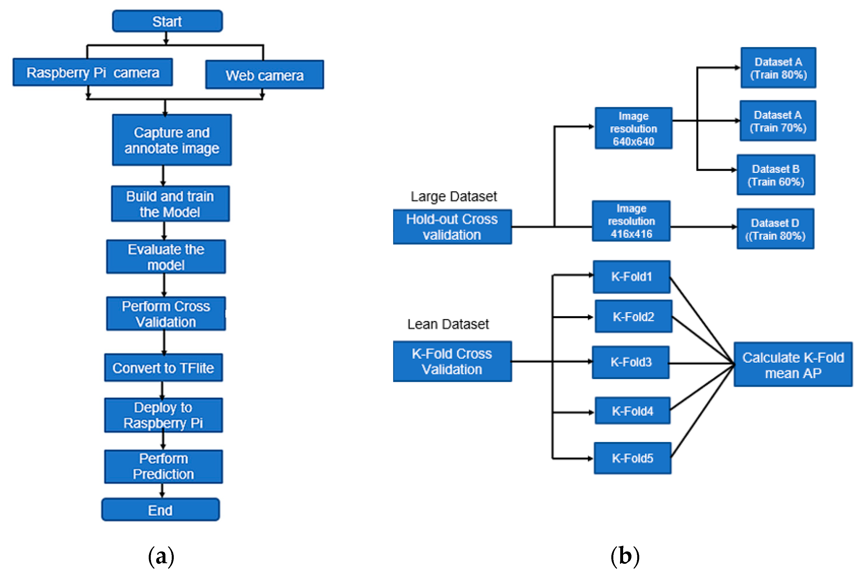
Figure 3 shows the cross-validation flow for Pick-and-Place solution using the Raspberry Pi. Using OpenCV on Raspberry Pi, the data images were captured, and the images were annotated using the online Roboflow tool. The dataset was then augmented and run on Google Colab for model building and training. This project used 2 strategies of cross-validation: Hold-out and K-Fold. The mean and variance AP of both strategies were calculated and compared. The detection scores, obtained from Raspberry Pi, were observed for a few minutes before the best values were recorded.
To run the python codes on Raspberry Pi, we created the virtual environment and used the detect.py file to detect custom object. A virtual environment was used to keep dependencies required by different projects separate. The filename must be set correctly so it will detect the containers.
Figure 4 shows the picture of the dataset. To allow generalization and prevent overfitting, 3 different background colours were used: black, brown, and white. The images of the containers were taken either separately or together, and they also have defects such as uneven colours and blurry or distorted conditions.
The TensorFlow model was developed and tested using Google Colab with Graphics Processing Unit (GPU) Hardware Accelerator. From TensorFlow, the model was converted to TensorFlow Lite, which is a production ready, cross-platform framework for deploying machine learning on mobile devices and embedded systems. The model was trained using a transfer learning method with a default learning rate 0.08. From our previous research [
17], a batchsize of 8 best represents the trade-off between speed and efficiency. Hence, for this project, we used a batchsize of 8, in line with our project’s goal of developing a machine vision assisted smart and lean Pick-and-Place system.
Using TensorFlow’s Model Maker, the model was built, trained, and evaluated before being converted to TensorFlow Lite. The lite version consumes less memory compared to the original version. Our evaluation criteria were the mean Average Precision (mAP) and F1-Score. For our Pick-and-Place application, the Recall was considered as Armax10, as we expected to have maximum 10 detections per Pick-and-Place application. The F1-score was used to evaluate the models’ accuracy since it allows for the simultaneous maximization of two metrics that are well-known in this field: Precision (which measures the detections of objects) and Recall (measures the objects that are detected). F1-score is calculated based on the mAP and Recall values in the formula below:
According to Raschka [
18], the Hold-out method for model evaluation and selection is not recommended when working with small datasets. Alternative methods for algorithm selection, such as the combined cross-validation, are recommended for comparing machine learning algorithms when datasets are small.
In machine learning, it is important to evaluate the bias and variance. Assuming there is a point estimator
of some parameter or function θ, the bias is commonly defined as the difference between the expected value of the estimator and the parameter that we want to estimate. The equation of bias:
If the bias is larger than zero, we also say that the estimator is positively biased. Conversely, if the bias is smaller than zero, the estimator is negatively biased. If the bias is exactly zero, the estimator is unbiased. The variance is defined as the difference between the expected value of the squared estimator minus the squared expectation of the estimator. It has its alternative form as:
To implement the cross-validation method of our smart and lean Pick-and-Place solution, we used a simple method for accuracy estimation; Hold-out with random resampling [
19] for a larger dataset, followed by a second method, K-Fold cross-validation, for a smaller dataset.
3.1. Hold-Out Validation Method
The Hold-out dataset consists of 793 original photos that have been brightened and exposed to create 1262 additional images, as shown in
Table 2. The effectiveness of this technique lies in the way neural networks understand the images and their characteristics. If an image is slightly altered, it is perceived by the network as a completely different image belonging to the same class.
To ensure equal distribution of workpieces in dataset, the project used Roboflow as an online annotation and data splitting tool. Using Label Assist tool in Roboflow, the highest mAP was used to annotate images and the confidence was lowered to 20%. The confidence level was lowered to make the annotation visible for all objects. The overlap was reduced to 50% to enable detection of workpiece with poor confidence. For faster annotation, the zoom and lock view functions were used to ensure more accurate annotation as the test objects looked bigger. For faster annotation, the functions zoom and lock view at 60% were used.
In total, this work uses 6 validation sets. Datasets A to D were used for Hold-out cross-validation while datasets E and F were used for K-Fold cross-validation. All the datasets were trained on EfficientDet 2 before conversion to EfficientDet-Lite2 for deployment on Raspberry Pi. The hyperparameters are shown in
Table 3.
Table 4 shows that there are 3 train/valid split ratios used in this work. Dataset A was set to 80:20 with the training set as 80% of the total images before augmentation. After augmentation, the train percentage was 92% and valid was 8% as the training images increased threefold. Dataset B had less original training images (70%) while Dataset C had the least original training images at 60%. Dataset D had a similar training split to Dataset A except that the input resolution was lower.
Table 5 shows the breakdown of the hold-out dataset into different colours. By ensuring the containers were equally distributed, the model is more robust and will not lead to overfitting. Other than this, other defects shown in
Table 6 such as container in flat orientation were added into the dataset.
3.2. K-Fold Cross-Validation Method
The second method used was K-Fold validation method on a smaller (leaner) dataset in order to produce more meaningful and reliable test result [
20]. In this method, the original dataset is randomly partitioned into k equal-size subsamples. In each case, each of the k subsamples is used as validation data and the remainder as training data. The stages in performing K-Fold cross-validation are described as follows:
- a.
Determine the number of K
- b.
Divide the data into 2 parts: train set and validation set
- c.
Obtain the evaluation results of model
- d.
Calculate the overall mean of the APs
In this project, we set K to be 5. Hence, the overall mean AP equation is:
For the 2 datasets shown in
Table 7, we used 2 different batchsizes and number of epochs as well as the input resolution.
Table 8 shows the breakdown of a smaller dataset used for the K-Fold cross-validation. Dataset2 has a total of 178 original images, augmented to 890 images. Similar to the Hold-out dataset, the photos were taken with 3 different backgrounds—black, brown, and white background.
For the K-Fold dataset, the pictures were taken using a Raspberry Pi 5 Megapixels camera. There are a total of 21 classes with 9 main classes, as shown in
Table 9. To make sure the system is more robust and will not lead to overfitting, other test objects with defects shown in such as the blue cube were added into the dataset, as shown in
Table 10.
4. Results of Hold-Out with Different Train/Valid/Test Split
The results in
Table 11 show that, not surprisingly, Dataset A with a higher train ratio has the highest AP (0.803) and Tflite AP (0.787). In contrast, Dataset C with a lower train ratio has the lowest AP (0.696) and Tflite AP (0.668). This is an expected result as the model is more accurate after training with more data. Compared to the baseline EfficientDet-Lite2 algorithm with mAP of 33.97%, our model improves the mean average precision (mAP) by 44.73% for Dataset A. The mAP increased by 32.9% for Dataset C with a 60% train split.
The results show that the light brown container has the highest overall mean AP value of 0.766 with the low variance value of 0.001240. The lowest variance 0.0008 is attained by the green container, which attains the second highest AP value of 0.755. This could be because strong colours and lighter tone colours offer strong contrast to the background and hence more features to the machine learning. In contrast, the dark blue container has the lowest mean AP of value 0.688, but with the highest variance at value 0.004323, which is more than three times higher than the light brown container.
Similarly, for detection scores shown in
Table 12 and
Figure 5, the lighter tone and strong-coloured containers have higher detection scores over the dark-coloured containers. Other than this, there are some misdetections due to the similar tone in colours. For example, the white colour is mistaken as gray on some detections. This could be prevented when more features are added into the container image, such as the corner castings. The corner castings are the big three-holed blocks which form the corners of all ISO shipping containers.
Figure 6 shows the loss function for Dataset A, which shows validation detection loss, box loss, class loss, and loss the lowest at epoch22. For comparison, we used Dataset B (
Figure 7), which shows similar validation detection loss, box loss, class loss, and loss the lowest at the epoch28, which is almost the mid run of the model. As the validation detection loss, box loss, and class loss are all at their lowest points in the middle of the total, this suggests that the model might be stopped sooner, leading to a leaner solution. This also suggests that Dataset A with a higher Train/Valid/Test split has faster convergence speed than Dataset B.
5. Results of K-Fold Validation
Table 13 shows the Average Precision of the K-Fold cross-validation for the model running on batchsize of 8 and epochs 80. A strong-coloured container such as a green container has a higher AP compared to a neutral-coloured container such as dark brown. The highest mean AP was obtained by the green container with a value 0.6662 while the dark brown container had the lowest mean AP value of 0.4036. Similar to the Hold-out dataset, a strong-coloured container offers more features compared to a neutral-coloured container especially when the background is of a similar coloured tone. More features in machine learning help improve the accuracy of machine learning models by allowing them to make more accurate predictions.
Table 14 shows the Average Precision of the K-Fold cross-validation for the model running on batchsize of 16 and epochs 100. A strong-coloured container such as the green container has a higher mean AP while a neutral dark-coloured container such as the dark brown has a lower mean AP. The highest mean was obtained by the green container with an AP value of 0.6832 while the dark brown container had the lowest mean AP value of 0.4002.
Table 15 shows the comparison of Average Precision for different K-Fold versions of the batchsize 8 with 80 epochs run and the batchsize 16 with 100 epochs run. The AP shows that the green container had the highest AP for both K-Fold versions while the dark brown had lowest AP for both datasets. Hence, higher contrast has more impact on the accuracy.
From
Figure 8, it is shown that the larger batchsize has a lower AP compared to the smaller batchsize. Compared to EfficientDet-Lite2’s mAP of 33.97%, the mAP for Dataset F increased by 6.29% while the mAP for Dataset E dropped by 1.01%.
In order to find out if there is any statistically significant difference between the two datasets in terms of Average Precision, we used the Mann–Whitney U test. According to [
21], the Mann–Whitney U test is the one of the most commonly used non-parametric statistical tests. This test was independently worked out by Mann and Whitney (1947) and it is a non-parametric test which is often used for small samples of non-normally distributed data [
22].
In the Mann–Whitney U test, the null hypothesis (H0) stipulates that the two groups come from the same population. In other terms, it stipulates that the two independent groups are homogeneous and have the same distribution. The alternative hypothesis (H1) against which the null hypothesis is tested stipulates that the first group data distribution differs from the second group data distribution.
In terms of medians, the null hypothesis states that the medians of the two respective samples are not different. As for the alternative hypothesis, it affirms that one median is larger than the other or quite simply that the two medians differ.
Therefore, if the null hypothesis is not rejected, it means that the median of each group of observations is similar. On the contrary, if the two medians differ, the null hypothesis is rejected. The two groups are then considered as coming from two different populations.
We applied the Mann–Whitney U test to our Datasets E and F as the number of classes are small, less than 30 [
23], and the AP results are not normally distributed. Below are our null and alternative hypotheses:
H0. The median of APs is equal between the two datasets.
H1. The median of APs is not equal between the two datasets.
Using SciPy which is a Python library used for scientific computing and technical computing, we obtained a p-value of 0.5745. Since the p-value (0.5745) is above than 0.05 significance level, we fail to reject the null hypothesis. We conclude there is not enough evidence to suggest a significant difference in medians between the 2 datasets.
Therefore, we can confirm that there is no significant difference between Dataset E and Dataset F in terms of Average Precision, despite having different batchsizes and number of epoch runs.
6. Comparison of EfficientDet-Lite with YOLOv4 Tiny and SSD MobileNet V2
To compare EfficientDet-Lite2 with other mobile-based object detection algorithms, we choose YOLOv4 Tiny and SSD MobileNet V2 FPNLite 320. YOLOv4 Tiny is a lightweight version of the YOLOv4 object detection model and SSD MobileNet V2 FPN 320 is a single-shot detection (SSD) model that uses the MobileNet V2 architecture as its backbone and a feature pyramid network (FPN) to improve performance.
Both algorithms are designed to be lightweight and suitable for implementation on edge devices. We used Dataset F to obtain the AP for these lightweight models with a learning rate of 0.08 and batchsize of 16. The AP results are shown in
Table 16 and the curves are plotted in
Figure 9. In terms of accuracy, YOLOv4 Tiny outperforms both EfficientDet-Lite2 and SSD MobileNet V2 FPN 320. SSD MobileNet has the lowest AP of 0.2975. The highest AP score among the three models is achieved by YOLOv4 Tiny on the white container, with a score of 0.8967. EfficientDet-Lite2 has the lowest AP score among the three models for most of the containers, except for the green container, where it has a slightly higher score than both models. SSD MobileNet shows lower mean AP due to the inability of the model to detect other classes, such as the red flat or red deformed container.
Overall, the results show that despite having a small dataset (Dataset F), the Average Precision across the three lightweight models is generally high as the models achieved more than 50% AP for the majority of the containers colours.
7. Conclusions
This work aims to improve the model performance by varying the train/valid/test split composition and image resolution, and evaluate the average precision and detection scores on different evaluation strategies. For the Hold-out dataset, the overall mean average precision increases as the train/test split ratio increases. Compared with the baseline EfficientDet-Lite2 algorithm, for Hold-out dataset, the mean average precision (mAP) is improved greatly by 40% with Average Precision (AP) of more than 80% and best detection scores of more than 93%. For K-Fold cross-validation for a small dataset with batchsize of 16, the mAP increased by 6.29% compared to the baseline model. Therefore, we conclude that using a training ratio of 80%, smaller batchsize, and lower image resolution will allow the network to train better. As shown in the loss graph, Dataset A achieved faster convergence than Dataset B. Coupled with the fact that the validation detection loss, box loss, and class loss are all at their lowest points in the middle of the total epochs is encouraging because it suggests that the model might be stopped sooner, leading to a leaner solution. The results show that despite having a lean K-Fold dataset, the Average Precision across the three lightweight models are generally high as the models achieved more than 50% AP for the majority of the containers colours. It was deduced that YOLOv4 Tiny was better than EfficientDet-Lite2 and SSD MobileNet V2 FPN 320 as a lightweight model, as a high value of precision was obtained while evaluating Dataset F.
For future works, we look at more precise container positioning. To locate the container on location, a camera must be positioned in a high spot. The size of each container will appear smaller as the camera’s height rises, lowering the object recognition system’s ability to accurately identify objects. At the actual site, however, the size of the container grows as the camera’s distance does, making recognition possible. We aim to create a machine vision system that can distinguish between the different container sizes and colours under conditions of varying illumination such as from morning to dawn. It is possible as well to increase the dataset using modern techniques such as dataset generation by 3D modelling software Blender 3.0 or Unity 2022.


