Parallelized A Posteriori Multiobjective Optimization in RF Design

Abstract

A posteriori multiobjective optimization relies on a series of mutually independent single-objective optimization subproblems, which can be run in parallel, thus making full use of a multiprocessor (or multicore) computer. This paper presents a parallel process launching scheme, such that practically no computing capacity gets wasted. This is achieved using standard Windows API kernel objects for process synchronization of the semaphore and mutex types. The algorithm used was further modified to inherently generate the desired Pareto front in the convenient form of a contour plot.

1. Introduction

One way of reducing computing time for multiobjective optimization consists in using efficient algorithms based on replacing the explored objective function with a less accurate but more easily computable surrogate objective function, as in [1,2,3,4]. Another way is parallelization, which is able to decrease the time even more, depending on the number of parallel processors. While many parallelization attempts have been used in the area of evolutionary multiobjective optimization algorithms [5,6,7,8,9,10,11] and other types of metaheuristics [12,13,14,15,16], we are utilizing our original multiobjective optimization method with an asymptotically uniform coverage of the Pareto front, which improves on [17,18,19,20,21] substantially. Part of the published research aims at using alternative computing platforms (GPUs, CUDA) [6,22,23]. However, our main objective dealt with in this paper was to develop a technical solution of synchronization of individual threads run in parallel to avoid collisions when accessing shared resources. It is an asynchronous task-launching scheme (in the meaning introduced in [24]), which allows for the restarting a new task immediately after any of the previously started ones finish, without having to wait for the end of all of the parallel runs. For generating tasks to be automatically distributed among a given number of simultaneously running processors (threads), we have efficiently used process synchronization objects.

The paper is organized as follows. In Section 2, we briefly specify our modification of the goal attainment method used as an a posteriori multiobjective optimization method. In Section 3, a method of solving obtained single-objective problems is defined in detail. Then, in Section 4, a way of utilizing our modification of method to generate a contour plot of the Pareto front is briefly proposed. Section 5 presents the parallelization scheme and explains its implementation using process synchronization objects. Finally, the application of the method is demonstrated on an example RF circuit designs in Section 6, Section 7, Section 8, Section 9 and Section 10, including appropriate graphical results and some comparison with other procedures.

2. Brief Description of a Posteriori Multiobjective Method

The purpose of multiobjective optimization (MO) is to solve the MO problem, i.e., to simultaneously minimize a set of k objective functions:

$$\underset{\mathit{x}\in S}{\mathrm{minimize}}\left\{g_1\left(\mathit{x}\right),g_2\left(\mathit{x}\right),\dots ,g_k\left(\mathit{x}\right)\right\},$$

(1)

where $\mathit{x}$ is the decision vector, $\mathit{x}={\left(x_1,x_2,\dots ,x_n\right)}^{\top }$. It is in the feasible region S, $S\subseteq {\mathsf{R}}^n$, which may be defined by a set of constraints and bounds on the decision variables $x_i$.

The above-mentioned requirement of simultaneous minimization translates as finding a single noninferior solution, which is an element of what is known as the Pareto front. A noninferior solution is such a solution in which an improvement in one objective is only possible at the cost of deteriorating at least one other objective. This means that a noninferior solution represents a certain tradeoff between mutually contradicting objectives. The choice of single solution is made in accordance with the decision maker’s (DM’s) preferences.

The class of a posteriori methods is defined by the fact that the DM’s preferences are applied on the resulting representation of the Pareto front only after its computation is finished. A posteriori MO methods can thus be considered as methods of obtaining and visualizing the Pareto front.

The a posteriori MO method used here is a modification of the goal attainment method. It converts the MO problem to a single-objective (SO) problem (SOP):

$$\underset{\mathit{x}\in S}{\mathrm{minimize}}\underset{i=1,\dots ,k}{max}\frac{g_i\left(\mathit{x}\right)-{\overline{z}}_i}{z_i^{\mathrm{nad}}-z_i^{\ast }},$$

(2)

where ${\overline{z}}_i$ stands for suitable reference goal values associated with the individual functions $g_i$. In the denominator of (2), $z_i^{\ast }$ are elements of the ideal (or best-case) vector ${\mathit{z}}^{\ast }=[z_1^{\ast },z_2^{\ast },\dots ,z_k^{\ast }]$ obtained by independent minimizations:

$${\mathit{z}}^{\ast }=\left[\underset{\mathit{x}\in S}{min}{g}_1\left(\mathit{x}\right),\underset{\mathit{x}\in S}{min}{g}_2\left(\mathit{x}\right),\dots ,\underset{\mathit{x}\in S}{min}{g}_k\left(\mathit{x}\right)\right].$$

(3)

Symbol $z_i^{\mathrm{nad}}$ represents a component of what is called the nadir (or worst-case) objective vector ${\mathit{z}}^{\mathrm{nad}}$, formed by the largest respective component ${\left({\mathit{z}}_i^{\ast }\right)}_j$ found in all k objective vectors ${\mathit{z}}_i^{\ast }$ obtained by independently minimizing the ith objective function:

$${\mathit{z}}^{\mathrm{nad}}=\left[\underset{i}{max}{\left({\mathit{z}}_i^{\ast }\right)}_1,\dots ,\underset{i}{max}{\left({\mathit{z}}_i^{\ast }\right)}_k\right].$$

(4)

The differences $z_i^{\mathrm{nad}}-z_i^{\ast }$ in the denominator of Equation (2) provide a convenient, automatically generated scaling of otherwise incommensurate components of the objective vector. (At a later stage, they may be manually adjusted by the user, e.g., to emphasize certain objectives over others.)

Let us now consider the selection of reference points $\overline{\mathit{z}}$. They can be used as a tool to greatly influence the location of the obtained solution, which is required so that the Pareto front is uniformly covered. In an attempt to approximately fulfill this requirement, $\overline{\mathit{z}}$ are (pseudo)randomly generated to uniformly cover a predefined reference set in the objective space formed by a convex body of k vertexes (a triangle if $k=3$, for instance):

$${\mathit{z}}_i^{\mathrm{vert}}={\left[z_1^{\mathrm{nad}},\dots ,z_{i-1}^{\mathrm{nad}},z_i^{\ast },z_{i+1}^{\mathrm{nad}},\dots ,z_k^{\mathrm{nad}}\right]}^{\top }\forall i=1,\dots ,k.$$

(5)

We proved that the following sequence of steps can be used to obtain such a reference point ${\mathit{z}}_{k-1,1}$:

$$\begin{array}{c}{t}_1=\sqrt[k-1]{r_1}\\ {\mathit{z}}_{1,1}=(1-t_1){\mathit{z}}_{0,1}+t_1{\mathit{z}}_{0,2}\\ {\mathit{z}}_{1,2}=(1-t_1){\mathit{z}}_{0,1}+t_1{\mathit{z}}_{0,3}\\ ⋮\\ {\mathit{z}}_{1,k-1}=(1-t_1){\mathit{z}}_{0,1}+t_1{\mathit{z}}_{0,k}\\ t_2=\sqrt[k-2]{r_2}\\ {\mathit{z}}_{2,1}=(1-t_2){\mathit{z}}_{1,1}+t_2{\mathit{z}}_{1,2}\\ {\mathit{z}}_{2,2}=(1-t_2){\mathit{z}}_{1,1}+t_2{\mathit{z}}_{1,3}\\ ⋮\\ {\mathit{z}}_{2,k-2}=(1-t_2){\mathit{z}}_{1,1}+t_2{\mathit{z}}_{1,k-1}\\ ⋮\\ t_{k-1}=\sqrt[1]{r_{k-1}}=r_{k-1}\\ {\mathit{z}}_{k-1,1}=(1-t_{k-1}){\mathit{z}}_{k-2,1}+t_{k-1}{\mathit{z}}_{k-2,2},\end{array}$$

(6)

where the starting points ${\mathit{z}}_{0,1}$ … ${\mathit{z}}_{0,k}$ are the vertices ${\mathit{z}}_1^{\mathrm{vert}}$ … ${\mathit{z}}_k^{\mathrm{vert}}$; and $r_i\in [0,1)$, $i=1,...,$$k-1$ are randomly generated real numbers uniformly distributed on interval $[0,1)$. The same can also be expressed in a more concise and “algorithmic” fashion as

$$\begin{array}{cc}\hfill & \mathtt{for}i=1\mathtt{to}k-1:\hfill \\ \hfill & t_i:=\sqrt[k-i]{r_i};\hfill \\ \hfill & \mathtt{for}j=1\mathtt{to}k-i:\hfill \\ \hfill & {\mathit{z}}_{i,j}:=(1-t_i){\mathit{z}}_{i-1,1}+t_i{\mathit{z}}_{i-1,j+1};\hfill \end{array}$$

(7)

N.B.: Equations (1)–(7) represent only a very brief description of our method. We already defined more comprehensive descriptions in [25,26,27], e.g., where certain comparisons with more other methods such as weighted Sum strategy, genetic, Nelder–Mead simplex, and simulated annealing algorithms were performed. However, as the main focus of this paper is devoted to the parallelization technique, we will not repeat such definitions and comparisons here, but we will thoroughly elaborate on the parallelization strategy instead.

3. Solving the SOP

To solve the obtained constrained single-objective problem, a derivative-based algorithm was adopted. As it is not meant to be the main focus of this paper, only a brief description will be provided here.

The algorithm is called sequential linear programming (SLP), a name formed by analogy to sequential quadratic programming (SQP). The central idea corresponds to the minimax method of paper [28], which resembles the method of approximate programming (MAP) [29] that also inspired some of the implemented features.

3.1. Form of Optimization Problem Solved

The SLP method solves constrained SOPs in the form

$$\underset{(\alpha ,\mathit{x})\in S}{\mathrm{minimize}}\alpha$$

(8)

where $\mathit{x}$ is the decision vector to be found, $\alpha$ is an auxiliary decision variable, and S is a feasible region, defined as

$$\begin{array}{cc}S=\{(\alpha ,\mathit{x})\in {\mathrm{R}}^{n+1}\mid & {\mathit{x}}_{\mathrm{l}}\leqq \mathit{x}\leqq {\mathit{x}}_{\mathrm{u}}\\ & \wedge -f_i\left(\mathit{x}\right)+a_{0i}\alpha \geqq 0\forall i\in I_1\\ & \wedge \phantom{-}{f}_i\left(\mathit{x}\right)\phantom{+a_{0i}\alpha }\geqq 0\forall i\in I_2\},\end{array}$$

(9)

with ${\mathit{x}}_{\mathrm{l}}$ and ${\mathit{x}}_{\mathrm{u}}$ being given vectors of lower and upper bounds for the components of decision vector $\mathit{x}$; $I_1$ being the set of all indexes i, such that $a_{0i}\ne 0$ (indexes of the components $f_i$ of an objective function to be minimized); and $I_2$ being the set of indexes i, such that $a_{0i}=0$ (indexes of constraint functions $f_i$ to be kept non-negative).

On closer inspection, this form of SOP can be obtained from form (2) by substitutions $f_i\left(\mathit{x}\right)=g_i\left(\mathit{x}\right)-{\overline{z}}_i$ and $a_{0i}=z_i^{\mathrm{nad}}-z_i^{\ast }$ for $i\in I_1$.

3.2. Algorithm Description

The top-level structure of the SLP algorithm can be roughly expressed as the following series of steps:

• Start at a given initial point $\mathit{x}={\mathit{x}}_0$.
• Evaluate the set of functions $f_i\left(\mathit{x}\right)$ and their derivatives $\partial f_i\left(\mathit{x}\right)/\partial x_j$.
• Test stopping condition and stop if it evaluates to true.
• Obtain new step $\Delta \mathit{x}$ by running the exchange algorithm for the linearized set of functions $f_i\left(\mathit{x}\right)$.
• Update vector $\mathit{x}$ with new iterate $max({\mathit{x}}_{\mathrm{l}},min({\mathit{x}}_{\mathrm{u}},\mathit{x}+\Delta \mathit{x}))$.
• Go to Step 2.

The result is then stored in the current decision vector $\mathit{x}$.

Now, we will give more details on the individual steps.

3.3. Linearized Form of the Problem

The linearized set of inequalities that is passed to the exchange algorithm in Step 4 is obtained from the values of functions $f_i$ and their derivatives obtained in Step 2:

$$\begin{array}{c}-f_i\left(\mathit{x}\right)+a_{0i}\alpha -{\displaystyle \sum _{j=1}^n}\frac{\partial f_i\left(\mathit{x}\right)}{\partial x_j}(\Delta x_j)\geqq 0\forall i\in I_1\\ f_i\left(\mathit{x}\right)\phantom{+a_{0i}\alpha }+{\displaystyle \sum _{j=1}^n}\frac{\partial f_i\left(\mathit{x}\right)}{\partial x_j}(\Delta x_j)\geqq 0\forall i\in I_2\end{array}$$

(10)

where $\Delta x_j$, $j=1,\dots ,n$ are the decision variables of the linear optimization problem, whose values are to be determined by the exchange algorithm.

3.4. Exchange Algorithm

The purpose of the exchange algorithm is to solve the linear constrained optimization problem. It is an extended version of the algorithm found in paper [28], where it is applied as part of an iterative minimax optimization method. The extensions are aimed at facilitating an inequality constraint mechanism to obtain a more general optimization routine. The algorithm implementation was also largely inspired by the implementation of the standard simplex algorithm of linear programming (LP), as published in [30].

The exchange algorithm is different from the simplex method of linear programming (LP) in that the decision variables can take both signs (in LP, they can only be non-negative), as well as being in the presence of an additional decision variable $\alpha$, which represents the value of the single linear objective function to be minimized.

Thus, several modifications have been performed in the effort to combine and extend the features of both of the algorithms, which can be summarized as follows:

• Allowing decision variables (including $\alpha$, an auxiliary variable representing the single-objective function value to be minimized) to take both signs;
• Also supporting negative and zero-valued coefficients of $\alpha$, so that constrained problems (i.e., with inequality constraints independent of $\alpha$) can be solved (as opposed to the pure unconstrained minimax problem);
• Implementing minimization of the objective function instead of maximization;
• Implementing special treatment to prevent infinite cycling in cases of degeneracies;
• Ensuring that all decision variables, including $\alpha$, are exchanged (and thus resolved).

3.5. Damping Step Sizes of Iterations

For the algorithm to be stable, it is necessary to limit the maximum size of steps in one iteration of each variable $\Delta x_j$. This is achieved by adding a pair of inequalities:

$$\begin{array}{c}min(s_{\mathrm{x}j},\mathit{x}-{\mathit{x}}_{\mathrm{l}})+\Delta x_j\geqq 0\\ min(s_{\mathrm{x}j},{\mathit{x}}_{\mathrm{u}}-\mathit{x})-\Delta x_j\geqq 0\end{array}$$

(11)

to (10) for each variable $\Delta x_j$, $j=1,\dots ,n$, with $s_{\mathrm{x}j}>0$ being a sufficiently small number. Note that the bounds on $\mathit{x}$ are enforced here rather than in Step 5.

3.6. Determining the Damping Step

In paper [28], the step size is limited by scaled value of $\alpha$. This is possible in the unconstrained minimax method if it is applied to problems where the objective function value (and thus, $\alpha$ as well) converges to zero or almost zero. In our case, a more flexible damping scheme needs to be used.

At the beginning, the values of maximum steps $s_{\mathrm{x}j}$ are given as input to the algorithm. After each iteration, they may be contracted (decreased), expanded (increased), or left unchanged.

Three possible strategies are implemented for contraction by a given coefficient $\chi$. The contraction can be chosen to be applied:

• Only if the change of $\Delta x_j$ changed its sign between the current and previous iteration;
• Or only if the objective function ${max}_{i\in I_1}{f}_i\left(\mathit{x}\right)$ has increased compared with its value before the last iteration;
• Or in either of the previous cases.

The contraction will happen only if the new step is still longer than $\epsilon (x_{\mathrm{u}j}-x_{\mathrm{l}j})/\chi$, where $\epsilon$ is the max. relative change used in the stopping criterion.

Expansion by coefficient $\sqrt[\kappa ]{\chi }$ (with $\kappa$ being a given parameter, typically 1 or 2) is always performed if the following conditions are simultaneously fulfilled:

• The change of $\Delta x_j$ changes its sign between the current and previous iteration;
• In both iterations, the particular damping constraint was active;
• The new step size is still shorter than its forbidden limit $(x_{\mathrm{u}j}-x_{\mathrm{l}j})/\left(\chi \sqrt[\kappa ]{\chi }\right)$.

3.7. Stopping Criterion

The iteration loop terminates as soon as the maximum relative change of all decision variables during the last $n_{\epsilon }$ iterations has not exceeded a given $\epsilon$ and the current iterate is feasible. However, if that has not happened during the first max_it iterations, the iterations are stopped after reaching a total of max_it iterations, where max_it is a given integer.

3.8. Modified Form of Constraints

If the given starting point ${\mathit{x}}_0$ is infeasible, the algorithm needs to find some feasible solution, and then it can proceed by optimizing it. The following modification of the constraint inequalities improves the chances of finding a feasible solution by the runs of the exchange algorithm:

$$f_i\left(\mathit{x}\right)-g+\alpha +\sum _{j=1}^n\frac{\partial f_i\left(\mathit{x}\right)}{\partial x_j}(\Delta x_j)\geqq 0\forall i\in I_2,$$

(12)

where

$$g=\underset{i\in I_1}{max}{f}_i\left(\mathit{x}\right)$$

(13)

is the objective function value in the current iterate $\mathit{x}$. This allows the $\alpha$ term in the constraints without significantly changing them, because typically, $\alpha \to g$ when vector $\mathit{x}$ approaches the optimum. (However, the step damping inequalities are still in action.)

This modification mode can be set as always on, on for finding the first feasible iterate only, or permanently switched off.

4. Contour Plot of a 3D Pareto Front

Let us now consider the possible ways of graphical presentation of an obtained Pareto front to the decision maker. If $k=2$, the Pareto front is a single curve in 2D and the case is trivial. For $k=3$, the Pareto front is formed by a surface in 3D objective space and is not as easy to display in a 2D plot. One way to distinguish the third dimension would be to define intervals and use different point symbols for each interval. Another option would be to use different shades of gray or different hues of colors.

A more sophisticated approach is a contour plot, where the optimization process is designed such that the obtained noninferior solutions are already concentrated in a vicinity of preselected values of the third objective, the contour parameter. For this purpose, one of the three objectives becomes an inequality constraint, and the simultaneous optimization of the remaining two objectives is repeated over individual values of the contour parameter. The individual sets of points obtained this way show the locations and shapes of underlying contour curves.

5. Process Parallelization Scheme

The computation of points forming the Pareto front is organized into two types of processes: a main process at the top level and a number of parallel processes subordinate to the main process.

5.1. Hierarchical Level of Parallelized Tasks

It is important to realize that the actual algorithm resulting from Section 2, Section 3 and Section 4 represents a multitude of nested loops (problem-oriented ones are located under the line):

• Going through a predefined list of contour parameter values;
  • Performing multiple SO runs to cover the current contour;
    • Iterations within each SO run;
      • Evaluations of objective functions and constraints to obtain their values and approximate their derivatives for each iteration;
        • Appropriate circuit analyses (typically running a circuit simulator) for each such evaluation;
          • … (The innermost levels are internal to the simulator and their number can vary widely, depending on types of analyses needed).
            Iterations of the scalar ϵ-algorithm (typically tens) when a steady-state period must be obtained (as they occurred in our RF-circuit design example)
            • Going through all points (typically hundreds or thousands) of the time response required in each iteration of the scalar ϵ-algorithm;
              • Going through all iterations (typically several or tens) of the Newton–Raphson method in each point of the time response;
                • Going through all columns (typically tens, hundreds, or thousands, depending on how large the circuit is) of the Jacobian matrix in the LU-factorization required in each iteration of the Newton–Raphson method—for extremely large circuits, this is the most demanding.

The level of subtasks that can be run in parallel needs to be chosen such that the subtasks are independent of each other, but are still as short as possible so that the waiting time to finish the running task is not too long. This is fulfilled by taking the whole single SO run for a single reference point as a unit task.

5.2. Process Synchronization Objects of the System Kernel

Now, the question is how to generate such tasks and distribute them automatically among a given number of simultaneously running processors. For this purpose, two types of process synchronization objects are used, called semaphore and mutex [31,32].

5.2.1. Semaphore

The semaphore is a special kind of a counter variable stored in the kernel memory space that can be used to organize access by multiple threads or processes to a shared system resource. This can be carried out due to a special treatment of a thread or process manipulating the counter’s content.

The creation of a new Semaphore object is performed using the function CreateSemaphore(), which also sets this variable to an non-negative initial value and takes an optional identification string. The initial value specifies how many threads/processes can simultaneously dispose of the particular system resource.

The semaphore gets decremented by calling the function WaitForSingleObject(), unless the value of the mutex is already zero. In such a case, the current thread/process is put to sleep. When the counter value becomes nonzero, one of the sleeping processes/threads wakes up, which also decrements the counter value back to zero.

The semaphore is incremented by means of the function ReleaseSemaphore(). This also wakes one of the currently sleeping threads/processes (due to the previous call of the WaitForSingleObject() function), if there are any.

5.2.2. Mutex

Mutex (whose name stands for mutually exclusive access) is essentially a special case of semaphore with a maximum value of one. This means that only one thread/process can dispose of the shared resource at a time (thus indeed providing it exclusive access).

Mutex is created by a call to the CreateMutex() API function, with an optional ID string as an argument. Access to the shared resource is granted by calling WaitForSingleObject(), which possibly enqueues the current thread/process by putting it to sleep if the mutex’s value is currently zero (indicating the protected resource currently being taken).

Mutex is incremented by a call to ReleaseMutex(), which subsequently wakes up one of sleeping threads/processes (if any).

5.3. The Main Process

The purpose of the main process is to run a batch of single-objective optimization runs as separate partially parallel subprocesses. Two thread synchronization objects are used here: a semaphore to limit the number of optimizations running in parallel to the number of available processor cores $N_{\mathrm{proc}}$ (e.g., 8 or 16); and a mutex enforcing exclusive access to the output NIS (noninferior solutions) file holding the achieved optimization results. The flowcharts of the main and paralell processes are shown in Figure 1 and Figure 2, respectively.

First, both the synchronization objects are created and initialized by calls to functions CreateSemaphore() and CreateMutex(). Moreover, an empty NIS file is created, so that it can be later appended with obtained noninferior optimization solution points.

Then two nested loops are used to launch individual parallel runs of the optimization process, each in its own working subdirectory, over the predefined list of contour parameter values $C_{\mathrm{list}}$ selected by the loop index i and for distinguishing values of the nested loop index j, enabling the pseudorandomly generated inputs of each of the parallel runs to be unique. Both loop indexes and the contour parameter value are passed to the individual parallel process in an input file called "INP", written in its subdirectory. Immediately after creating each parallel process, its process and thread handles can be closed by calls to CloseHandle(), as they are no longer needed in the main process.

After the whole of the intended number of parallel processes have been launched, most of them have already finished, but the final batch of $N_{\mathrm{proc}}$ is still running. Therefore, the main process waits for all of them to finish using yet another loop, this time controlled by the p parameter. Then, it can close its semaphore and mutex handles, and thus allow the operating system to free both of the synchronizing objects. After that, the main process itself closes down. The resulting set of noninferior solutions is gathered in the NIS file and is ready for inspection.

Note that no processor (core) apart from the $N_{\mathrm{proc}}$ total needs to be specifically reserved for the main process itself because it spends most of the time sleeping and waiting for any of the running processes to finish, and thus, its overall computational demand turns out to be negligible.

5.4. The Parallel Process

After a parallel subprocess is created by the main process, the INP file in the current working subdirectory is open and both loop parameters are read from it. Then, objective reference point $z_{\mathrm{ref}}$ and initial iterate $x_0$ are generated with a pseudorandom generator. A simple mapping function, e.g., $f_{\mathrm{s}}(i,j)=i\times \mathrm{10,000}+j$, is used to obtain a randomizing seed value.

Then, a single-objective optimization solver is used to try to find a solution to the problem (2). If a feasible solution x has been found, exclusive access to the shared output NIS file is obtained via waiting for mutex. The file is read and rewritten, with x being included to it if it is found noninferior with respect to the current NIS file content. (In this process, some of the existing solutions may be also removed from the NIS file if they happen to be found inferior to the new x). After this operation and closing the NIS file, the mutex is released and its handle closed, and the current working subdirectory is emptied and removed. (The updated NIS file remains in the parent directory one level of nesting above. This way, the NIS file always holds a set of mutually noninferior solutions.) After releasing the semaphore and closing its handle, the parallel subprocess is ready to finish.

6. Example Application in RF Circuit Design

For an example, a basic design of the end stage of an narrow-band RF power amplifier at $f_1=300\mathrm{MHz}$ is chosen. Source and load impedances are both $50\Omega$ and supply voltage $V_{\mathrm{dd}}=12\mathrm{V}$. The aim is to show the available tradeoffs between output power, power efficiency, and total harmonic distortion.

6.1. Circuit Schematic

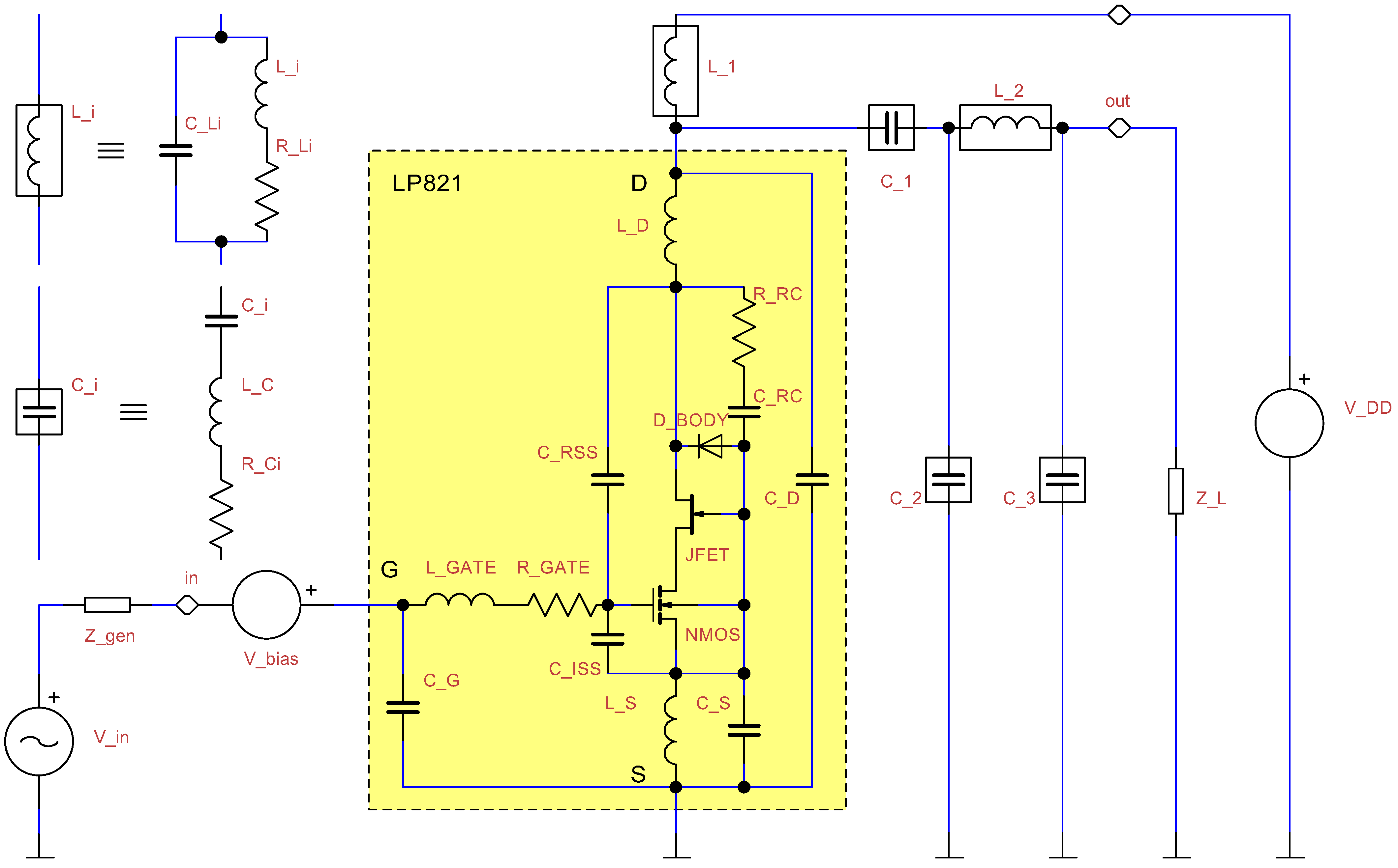
The simulation schematic is based on a silicon N-channel LDMOS device LP821 (Polyfet RF Devices) of a maximum total dissipated power of $50$W and a topology that is typical for the C-class mode of operation; see Figure 3. The transistor is followed by an LC filter to diminish higher harmonic components and provide a good impedance matching. (Even though impedance matching at the output is not directly required, it is enforced indirectly by maximizing output power.)

Note that the elements $C_1$, $C_2$, and $L_1$ can also be considered as a form of a tapped resonant circuit. The maximum operating frequency of the Polyfet LDMOS transistor can be $500$MHz, which is well above the design band of this power amplifier.

We want to explore the output trade-offs rather than obtaining a complete design. Please also note that no input impedance matching circuit is considered, and no stability-ensuring measures are taken (with the exception of the small reactance of the capacitance between the source and gate of the transistor itself).

6.2. Design Variables

The set of all design variables is formed by two groups. The first one specifies the transistor’s gate voltage, and thus its mode of operation; the second group are values of the output filter’s LC components.

The first design variable was chosen to be an estimated peak $V_{\mathrm{gs}\max }$ of the gate voltage $V_{\mathrm{gs}}$. The second one is its AC component magnitude $V_{\mathrm{gsACm}}$, related to input voltage magnitude $V_{\mathrm{inACm}}$ via the voltage dividing ratio between a driving resistance $R_{\mathrm{d}}$ and the gate capacitive reactance approximated as 10 ohms:

$$V_{\mathrm{gsACm}}=V_{\mathrm{inACm}}\frac{X_{\mathrm{i}}}{\sqrt{X_{\mathrm{i}}^2+R_{\mathrm{d}}^2}},$$

(14)

From this, we obtain the DC and AC voltage source values in Figure 3:

$$V_{\mathrm{bias}}=V_{\mathrm{gs}\max }-V_{\mathrm{gsACm}}\mathrm{and}{V}_{\mathrm{inACm}}=V_{\mathrm{gsACm}}\frac{\sqrt{X_{\mathrm{i}}^2+R_{\mathrm{d}}^2}}{X_{\mathrm{i}}}.$$

(15)

This arrangement allows limiting the peak gate voltage simply by an upper bound on $V_{\mathrm{gs}\max }$ to its maximum rating value (rather than performing it by means of an additional inequality constraint on the gate voltage).

The parameters of stray phenomena of the L and C component models shown in Figure 3 are obtained as mere estimates in a simple (but nontrivial) manner depending on the components’ principal L/C values.

Table 1. Design variables for the power amplifier.

		Bound			Coverage
No.	Symbol	Lower	Upper	Unit	Type
1	$V_{\mathrm{gs}\max }$	2	20	V	linear
2	$V_{\mathrm{gsACm}}$	0.4	12	V	linear
3	$L_1$	3	30	nH	logarithmic
4	$C_1$	10	300	pF	logarithmic
5	$C_2$	3	300	pF	logarithmic
6	$L_2$	3	100	nH	logarithmic
7	$C_3$	3	100	pF	logarithmic

contains a complete list of the design variables for the multiobjective optimization process. (The ranges are chosen by a user with respect to the intended practical realization of the amplifier. The “Coverage type” field specifies whether the random generator of the initial iterate uniformly covers the specified range on a linear or logarithmic scale.)

6.3. Design Goals

Our MO problem amounts to five design goals: three simultaneously optimized objective functions and two constraints based on selected absolute maximum ratings of the transistor. All of the goals are evaluated from voltages and currents provided by the steady-state (SS) analysis of the simulator CIA.

Table 2. Design Goals for the power amplifier. (THD has the preselected values of the objective, the contour parameter).

				Optimum
No.	Symbol	Type	Direction	or Bound	Unit
1	$P_{\mathrm{out}1}$	objective	maximum	32.137826	W
2	$\eta$	objective	maximum	81.680676	%
3	THD	objective	minimum	set to0.25	%
4	$I_{\mathrm{d}\mathrm{avg}}$	constraint	≦	5	A
5	$P_{\mathrm{diss}}$	constraint	≦	50	W

lists all design goals. Their definitions are:

• Average output power at the first harmonic frequency $P_{\mathrm{out}1}$

$$P_{\mathrm{out}1}=\frac{|{\mathit{v}}_{\mathrm{out}1}{|}^2}{2R_{\mathrm{L}}}=\frac{a_1^2+b_1^2}{2R_{\mathrm{L}}},$$

(16)

where ${\mathit{v}}_{\mathrm{out}1}$ is the phasor of the output voltage $v_{\mathrm{out}}\left(t\right)$; $a_k$ and $b_k$ are the coefficients of the k-th cosine and sine harmonic series components of the periodic steady-state output voltage $v_{\mathrm{out}}\left(t\right)$ of the period T:

$$a_k=\frac{2}{T}\underset{T}{\int }{v}_{\mathrm{out}}\left(t\right)cos\frac{2\pi }{T}tdt\mathrm{and}{b}_k=\frac{2}{T}\underset{T}{\int }{v}_{\mathrm{out}}\left(t\right)sin\frac{2\pi }{T}tdt.$$

(17)

The integrals over period T are computed with the trapezoid method of numeric integration.

• Power efficiency $\eta$, defined as the ratio of output power at the first harmonic frequency and the sum of average power from DC power supply and power from the (imaginary) input driving stage. (This definition pushes not only for lower power dissipation on the transistor, but also for lower input power, and thus for higher power gain.)
• Total harmonic distortion THD of the output voltage $v_{\mathrm{out}}\left(t\right)$ in %. Although this goal is considered a minimized objective, it was chosen as the contour parameter and thus changed into an inequality constraint, as explained in Section 3.
• Average drain current $I_{\mathrm{d}\mathrm{avg}}$ representing the supply current consumption of the power amplifier, chosen to be kept below $5\mathrm{A}$.
• Dissipated power of the LDMOS transistor $P_{\mathrm{diss}}$, representing the undesirable power loss, and chosen to be kept below $50\mathrm{W}$.

6.4. Obtained Contour Plot

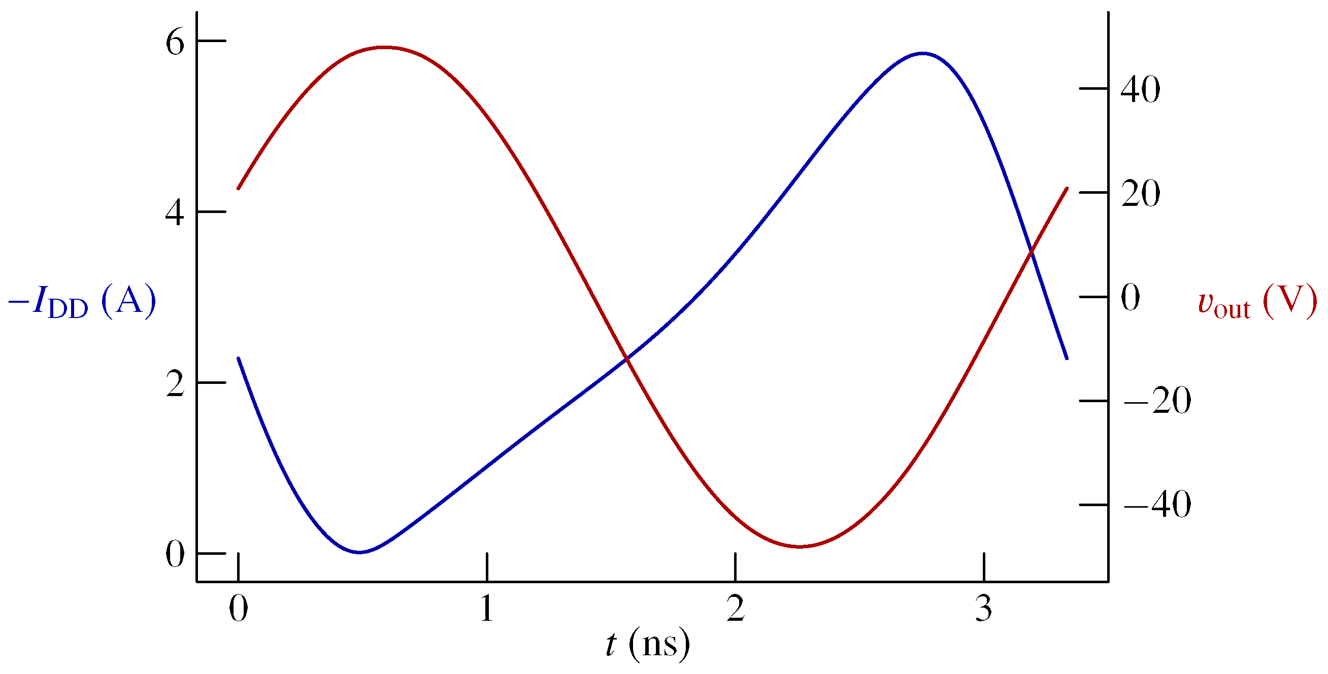
The resulting contour plot of the analyzed Pareto front is shown in Figure 4. The chosen levels of total harmonic distortion were chosen so that the shape of the 3D surface can be easily envisioned. Moreover, typical results for a chosen point are shown in Figure 5.

7. A Note on the Usage of the Method in the Frequency Domain

We thoroughly tested the algorithm on analyses in frequency domain as well [25,26,27], including two-, three-, and even four-dimensional examples. However, it should be stated that the computations in the frequency domain are (much) simpler than those in the time domain. Please note that in the problem-oriented loops described in Section 5.1, there are only two levels here (instead of four levels necessary in the time domain):

• Going through all required frequencies (typically tens or hundreds);
  • Going through all columns of the Jacobian matrix in complex LUfactorization.

Although the complex LU factorization is more difficult than the real one, the computational effort is clearly much lower than that in the time domain. Therefore, in the frequency domain, the parallelization is much less urgent than in the time domain.

8. Another Example: Four-Dimensional Problem

In this section, we will provide another design example to show a comparison of two different methods in pursuing the same task of exploring a Pareto front, this time in a four-dimensional objective space. The circuit to be optimized is an amplifier of a video signal in Figure 6, whose input should be matched to $75\Omega$, and output driving a $75\Omega$ load to at least $1{\mathrm{V}}_{\mathrm{pp}}$ of voltage span. Remaining parameters of interest are the low-frequency voltage gain $A_{\mathrm{v}}$ and 3 dB roll-off frequency $f_m$ to be maximized and total DC current supply $I_{\mathrm{cc}}$ to be minimized. There will be a total of five design variables: the resistances $R_1$–$R_5$. The capacitances $C_1$–$C_3$ will be assumed high enough to have negligible impact on the gain at low frequencies. Transistor type is 2N5179, same for both $Q_1$ and $Q_2$. The requested input impedance matching will be characterized by a standing voltage ratio $\mathrm{SWR}=(1+|\rho \left|\right)/(1-|\rho \left|\right)$, where $\rho =(R_{\mathrm{i}}-75\Omega )/(R_{\mathrm{i}}+75\Omega )$.

The above specifications lead to the multiobjective optimization problem

$$\begin{array}{cccc}\hfill & \mathrm{minimize}\hfill & \hfill & \mathrm{SWR},I_{\mathrm{cc}},\hfill \\ \hfill & \mathrm{maximize}\hfill & \hfill & A_{\mathrm{vdB}},f_{\mathrm{m}}\hfill \\ \hfill & \mathrm{subject}\mathrm{to}\hfill & \hfill & V_{\mathrm{out}}\leqq 3.5\mathrm{V},\hfill \end{array}$$

(18)

where the constraint condition on $V_{\mathrm{out}}$ implements the requirement of $1{\mathrm{V}}_{\mathrm{pp}}$ minimum guaranteed output voltage span.

Both the weighted sum strategy (WSS) and goal attainment method (GAM) have been used to solve the problem (18).

8.1. Weighted Sum Strategy

The following set of objective functions to be minimized was chosen:

$${\displaystyle f_1=10(\mathrm{SWR}-1),f_2=A_{\mathrm{vdB}}^{\mathrm{o}}-A_{\mathrm{vdB}},f_3=\frac{I_{\mathrm{cc}}}{1\mathrm{mA}},f_4={log}_{10}\frac{f_{\mathrm{m}}^{\mathrm{o}}}{f_{\mathrm{m}}},}$$

(19)

where $A_{\mathrm{vdB}}^{\mathrm{o}}=40.72\mathrm{dB}$ and $f_{\mathrm{m}}^{\mathrm{o}}=860.3\mathrm{MHz}$ are independently optimized results for the voltage gain $A_{\mathrm{vdB}}$ and the roll-off frequency $f_{\mathrm{m}}$, respectively.

The constrained optimization problem is converted into an unconstrained one using the penalty function method. The penalty function added to a single-objective function is as follows:

$$c_1=max\left(\frac{V_{\mathrm{out}}-3.5\mathrm{V}}{3.5\mathrm{V}},0\right)\times q.$$

(20)

The emphasis on the constraint term is controlled by the coefficient q, $q=100$. The scalar objective function to be minimized can be expressed as

$$f_{\mathrm{P}}\left(\mathit{x}\right)=\sum _{i=1}^4{w}_i{f}_i^2\left(\mathit{x}\right)+c_1^2\left(\mathit{x}\right)$$

(21)

where the choice of weight values is further restricted with the usual condition ${\sum }_{i=1}^4{w}_i=1$.

To minimize the objective function $f_{\mathrm{P}}$, our special version of the Levenberg–Marquardt method was used (which normalizes the Jacobian matrix). Iterations end after the biggest relative change in the design variables between iterations becomes smaller than ${10}^{-4}$ or when a maximum allowed number of iterations is reached.

8.2. Goal Attainment Method

The individual objective functions $f_i$ and the constraint penalty function $c_1$ are the same. However, in the GAM method, they change into a single-objective function to be minimized, which is $f\left(\mathit{x}\right)=\gamma$; and the following set of constraint penalty functions, $q=100$:

$$\begin{array}{ccc}\hfill g_1& =& {\displaystyle max\left(\frac{10(\mathrm{SWR}-1)-w_1\gamma -P}{P},0\right)\times q,}\hfill \\ \hfill g_2& =& {\displaystyle max\left(\frac{A_{\mathrm{vdB}}^{\mathrm{o}}-A_{\mathrm{vdB}}-w_2\gamma -P}{P},0\right)\times q}\hfill \\ \hfill g_3& =& {\displaystyle max\left(\frac{I_{\mathrm{cc}}/1\mathrm{mA}-w_3\gamma -P}{P},0\right)\times q,}\hfill \\ \hfill g_4& =& {\displaystyle max\left(\frac{{log}_{10}\left(f_{\mathrm{m}}^{\mathrm{o}}/f_{\mathrm{m}}\right)-w_4\gamma -P}{P},0\right)\times q}\hfill \end{array}$$

(22)

complemented with the original constraint penalty function $c_1$. Note that to reduce the number of degrees of freedom, we set all the reference goals ${\overline{z}}_i$ equal to the same scalar value P, $P=10$. This is possible because of the special choice of objective functions $f_i$. The resulting scalar objective function to be minimized is then composed as follows:

$$f_{\mathrm{P}}\left(\mathit{x}\right)={\gamma }^2+\sum _{i=1}^4{g}_i^2\left(\mathit{x}\right)+c_1^2\left(\mathit{x}\right).$$

(23)

The same procedure using the Levenberg–Marquardt method is applied to obtain solutions for chosen values of $w_i$ and P as that with WSS.

8.3. Results Obtained with Weighted Sum Strategy (Table 3)

Multiple optimization runs were tried for different sets of weighting coefficients $w_i$. The result obtained by minimizing the composed scalar objective function also gives the four design goals: $\mathrm{SWR}$, $A_{\mathrm{vdB}}$, $I_{\mathrm{cc}}$, and $f_{\mathrm{m}}$. In the table, they are listed in the same order as their respective weights $w_i$ are. Therefore, the effect of changing a weighting coefficient can be easily examined. For instance, increasing $w_1$ in row No. 2 decreases the value of $\mathrm{SWR}$ compared to row No. 1, decreases $A_{\mathrm{v}}$, and decreases $I_{\mathrm{cc}}$. We would expect an improvement in the goal whose weight has increased, but disimprovement in the remaining goals. This is also what happened, with the only exception being $I_{\mathrm{cc}}$.

This is expressed by the “success rate” $S_1$ value of $75\%$. (The subscript of “1” in $S_1$ refers to the reference row with respect to which the changes are evaluated.) We can also see that the average value of $S_1$ of $62.5\%$ is well above $50\%$.

Moreover, the noninferiority of the obtained data was tested. This is a test for each solution in the table to see whether no other solution in the table has all of its components of better values (in terms of the design assignment) than the one tested. This is a necessary condition for any valid candidate for a noninferior solution. Each of the nine solutions passed this test.

Table 3. Results obtained by weighted sum strategy.

					SWR	${\mathit{A}}_{\mathbf{v}}$	${\mathit{I}}_{\mathbf{cc}}$	${\mathit{f}}_{\mathbf{m}}$	${\mathit{S}}_{\mathbf{1}}$
No.	${\mathit{w}}_{\mathbf{1}}$	${\mathit{w}}_{\mathbf{2}}$	${\mathit{w}}_{\mathbf{3}}$	${\mathit{w}}_{\mathbf{4}}$	(–)	(dB)	(mA)	(MHz)	(%)
1	0.25	0.25	0.25	0.25	1.02	40.1	0.486	128	–
2	0.4	0.2	0.2	0.2	1.00	40.0	0.485	127	75
3	0.2	0.4	0.2	0.2	1.02	40.1	0.479	126	75
4	0.2	0.2	0.4	0.2	1.01	40.3	0.376	112	50
5	0.2	0.2	0.2	0.4	1.02	40.0	0.487	128	50
6	0.7	0.1	0.1	0.1	1.00	40.0	0.478	125	75
7	0.1	0.7	0.1	0.1	1.07	40.2	0.481	128	50
8	0.1	0.1	0.7	0.1	1.00	40.2	0.311	94.3	50
9	0.1	0.1	0.1	0.7	1.03	40.1	0.488	128	75
Single-run average correlation					62.5	62.5	50.0	75.0	62.5

Table 3. Results obtained by weighted sum strategy.

					SWR	${\mathit{A}}_{\mathbf{v}}$	${\mathit{I}}_{\mathbf{cc}}$	${\mathit{f}}_{\mathbf{m}}$	${\mathit{S}}_{\mathbf{1}}$
No.	${\mathit{w}}_{\mathbf{1}}$	${\mathit{w}}_{\mathbf{2}}$	${\mathit{w}}_{\mathbf{3}}$	${\mathit{w}}_{\mathbf{4}}$	(–)	(dB)	(mA)	(MHz)	(%)
1	0.25	0.25	0.25	0.25	1.02	40.1	0.486	128	–
2	0.4	0.2	0.2	0.2	1.00	40.0	0.485	127	75
3	0.2	0.4	0.2	0.2	1.02	40.1	0.479	126	75
4	0.2	0.2	0.4	0.2	1.01	40.3	0.376	112	50
5	0.2	0.2	0.2	0.4	1.02	40.0	0.487	128	50
6	0.7	0.1	0.1	0.1	1.00	40.0	0.478	125	75
7	0.1	0.7	0.1	0.1	1.07	40.2	0.481	128	50
8	0.1	0.1	0.7	0.1	1.00	40.2	0.311	94.3	50
9	0.1	0.1	0.1	0.7	1.03	40.1	0.488	128	75
Single-run average correlation					62.5	62.5	50.0	75.0	62.5

8.4. Results Obtained with Goal Attainment Method (Table 4)

Similarly to the previous case of WSS, the coefficients $w_i$ of GAM are also used in the attempts to steer the location of found solutions onto (or close to) the Pareto front. Increasing $w_i$ usually allows for larger changes of the respective objective in the required direction. Therefore, increasing any $w_i$ should improve the objective value.

The resulting average correlation rate of 79.2% looks much better than that of the WSS. A noninferiority test was also performed, and all the solutions in the table passed.

All noninferior solutions found were used to generate an interpolated estimate of the 4-dimensional Pareto front, as in the quasi four-dimensional plots in Figure 7.

Table 4. Results obtained by goal attainment method.

					SWR	${\mathit{A}}_{\mathbf{v}}$	${\mathit{I}}_{\mathbf{cc}}$	${\mathit{f}}_{\mathbf{m}}$	${\mathit{S}}_{\mathbf{1}}$
No.	${\mathit{w}}_{\mathbf{1}}$	${\mathit{w}}_{\mathbf{2}}$	${\mathit{w}}_{\mathbf{3}}$	${\mathit{w}}_{\mathbf{4}}$	(–)	(dB)	(mA)	(MHz)	(%)
1	1	1	1	1	1.07	40.0	0.505	134	–
2	1	0	0	0	1.00	32.4	0.844	302	75
3	0	1	0	0	1.18	40.5	0.477	129	75
4	0	0	1	0	1.63	30.7	0.404	174	75
5	0	0	0	1	1.67	30.7	1.780	583	100
6	2	1	1	1	1.00	38.9	0.973	131	100
7	1	2	1	1	1.18	40.5	0.477	129	75
8	1	1	2	1	1.18	35.6	0.463	154	75
9	1	1	1	2	1.48	35.5	0.848	296	100
10	2	2	2	1	1.06	40.1	0.491	130	100
11	2	2	1	2	1.05	40.0	0.491	130	25
12	2	1	2	2	1.02	35.5	0.500	203	100
13	1	2	2	2	1.12	40.0	0.477	129	50
Single-run average correlation					95.5	86.4	68.2	72.7	79.2

Table 4. Results obtained by goal attainment method.

					SWR	${\mathit{A}}_{\mathbf{v}}$	${\mathit{I}}_{\mathbf{cc}}$	${\mathit{f}}_{\mathbf{m}}$	${\mathit{S}}_{\mathbf{1}}$
No.	${\mathit{w}}_{\mathbf{1}}$	${\mathit{w}}_{\mathbf{2}}$	${\mathit{w}}_{\mathbf{3}}$	${\mathit{w}}_{\mathbf{4}}$	(–)	(dB)	(mA)	(MHz)	(%)
1	1	1	1	1	1.07	40.0	0.505	134	–
2	1	0	0	0	1.00	32.4	0.844	302	75
3	0	1	0	0	1.18	40.5	0.477	129	75
4	0	0	1	0	1.63	30.7	0.404	174	75
5	0	0	0	1	1.67	30.7	1.780	583	100
6	2	1	1	1	1.00	38.9	0.973	131	100
7	1	2	1	1	1.18	40.5	0.477	129	75
8	1	1	2	1	1.18	35.6	0.463	154	75
9	1	1	1	2	1.48	35.5	0.848	296	100
10	2	2	2	1	1.06	40.1	0.491	130	100
11	2	2	1	2	1.05	40.0	0.491	130	25
12	2	1	2	2	1.02	35.5	0.500	203	100
13	1	2	2	2	1.12	40.0	0.477	129	50
Single-run average correlation					95.5	86.4	68.2	72.7	79.2

9. Testing Processor Exploitation

The efficiency of the whole parallelized procedure can be well illustrated by XMeters graphs of the exploitation of the cores/threads of a processor. In Figure 8, the exploitation of the threads is shown in the cases of one, two, …, or eight parallel processes of our multiobjective procedure that ran on the Intel Core i7-860 processor (four cores, eight threads). The (very small) red-colored amount represents system (Windows) demands; the violet columns represent the demands of our multiobjective procedure. It is clear that for eight processes computed in parallel (the last picture at the end), practically the whole capacity of the processor is exploitable, which confirms our strategy very well.

10. Note on Another Recently Published Example: Ultra-Low-Noise Antenna Amplifier

We thoroughly tested our algorithm on the multiobjective optimization of an ultra-low-noise antenna amplifier for all five (GPS, GLONASS, BeiDou, Galileo, and NavIC) satellite navigation systems. A comparison of the single- and multiband realizations was published in [27], where the optimized and measured results for the noise figure and amplification of the two variants were compared (as well as necessary stability tests) for the two variants. The new measured method was published in [33], where a comparison of the computed and measured transducer power gain was performed as well. Therefore, this example can be considered another confirmation of the full functionality of our method and related software procedures.

11. Conclusions

The following achievements described in the paper deserve to be highlighted:

• Our modification of the a posteriori goal attainment method has been devised and presented, which leads to asymptotically uniform coverage of the reference set by chosen reference points used to control the exploration of Pareto front.
• Regarding actual computation strategy, a way of parallel processing has been chosen, such that the tasks run in parallel are automatically started one after another on each of the available processor cores without any slack time needed, contrary to many other published procedures. This is due to the specific organizing role of the main process starting the child processes.
• The resulting graph Figure 4 in the form of contour plot is more informative of the actual Pareto front shape than other frequently used forms of depiction in literature.

References

- de Winter, R.; Bronkhorst, P.; van Stein, B.; Bäck, T. Constrained Multi-Objective Optimization with a Limited Budget of Function Evaluations. Memetic Comput. 2022, 14, 151–164. [Google Scholar] [CrossRef]
- Akhtar, T.; Shoemaker, C.A. Efficient multi-objective optimization through population-based parallel surrogate search. arXiv 2019, arXiv:1903.02167. [Google Scholar]
- Zhang, S.; Yang, F.; Yan, C.; Zhou, D.; Zeng, X. An Efficient Batch-Constrained Bayesian Optimization Approach for Analog Circuit Synthesis via Multiobjective Acquisition Ensemble. IEEE Trans. Comput.-Aided Des. Integr. Circuits Syst. 2021, 41, 1–14. [Google Scholar] [CrossRef]
- Lyu, W.; Yang, F.; Yan, C.; Zhou, D.; Zeng, X. Batch Bayesian optimization via multi-objective acquisition ensemble for automated analog circuit design. In Proceedings of the International Conference on Machine Learning, Stockholm, Sweden, 10–15 July 2018; pp. 3306–3314. [Google Scholar]
- Deb, K.; Sundar, J. Reference point based multi-objective optimization using evolutionary algorithms. In Proceedings of the 8th Annual Conference on Genetic and Evolutionary Computation, New York, NY, USA, 8–12 July 2006; pp. 635–642. [Google Scholar]
- Gupta, S.; Tan, G. A scalable parallel implementation of evolutionary algorithms for multi-objective optimization on GPUs. In Proceedings of the 2015 IEEE Congress on Evolutionary Computation (CEC), Sendai, Japan, 25–28 May 2015; pp. 1567–1574. [Google Scholar]
- Zhang, K.; Chen, M.; Xu, X.; Yen, G.G. Multi-objective evolution strategy for multimodal multi-objective optimization. Appl. Soft Comput. 2021, 101, 107004. [Google Scholar] [CrossRef]
- Kimovski, D.; Ortega, J.; Ortiz, A.; Baños, R. Parallel alternatives for evolutionary multi-objective optimization in unsupervised feature selection. Expert Syst. Appl. 2015, 42, 4239–4252. [Google Scholar] [CrossRef]
- Saravana Sankar, S.; Ponnambalam, S.; Gurumarimuthu, M. Scheduling flexible manufacturing systems using parallelization of multi-objective evolutionary algorithms. Int. J. Adv. Manuf. Technol. 2006, 30, 279–285. [Google Scholar] [CrossRef]
- Tian, Y.; Si, L.; Zhang, X.; Cheng, R.; He, C.; Tan, K.C.; Jin, Y. Evolutionary large-scale multi-objective optimization: A survey. ACM Comput. Surv. (CSUR) 2021, 54, 1–34. [Google Scholar] [CrossRef]
- Belaiche, L.; Kahloul, L.; Benharzallah, S. Parallel Dynamic Multi-Objective Optimization Evolutionary Algorithm. In Proceedings of the 2021 22nd International Arab Conference on Information Technology (ACIT), Muscat, Oman, 21–23 December 2021; pp. 1–6. [Google Scholar]
- Alba, E.; Luque, G.; Nesmachnow, S. Parallel metaheuristics: Recent advances and new trends. Int. Trans. Oper. Res. 2013, 20, 1–48. [Google Scholar] [CrossRef]
- Benítez-Hidalgo, A.; Nebro, A.J.; García-Nieto, J.; Oregi, I.; Del Ser, J. jMetalPy: A Python framework for multi-objective optimization with metaheuristics. Swarm Evol. Comput. 2019, 51, 100598. [Google Scholar] [CrossRef]
- Blank, J.; Deb, K. Pymoo: Multi-objective optimization in python. IEEE Access 2020, 8, 89497–89509. [Google Scholar] [CrossRef]
- Li, X.; Gao, B.; Bai, Z.; Pan, Y.; Gao, Y. An improved parallelized multi-objective optimization method for complex geographical spatial sampling: AMOSA-II. ISPRS Int. J. Geo-Inf. 2020, 9, 236. [Google Scholar] [CrossRef]
- Nemura, M. Parallelization of Multi-Objective Optimization Methods. Ph.D. Thesis, Vilniaus Universitetas, Vilnius, Lithuania, 2021. [Google Scholar]
- Miettinen, K. Nonlinear Multiobjective Optimization; Springer Science & Business Media: Berlin/Heidelberg, Germany, 2012; Volume 12. [Google Scholar]
- Figueira, J.R.; Liefooghe, A.; Talbi, E.G.; Wierzbicki, A.P. A parallel multiple reference point approach for multi-objective optimization. Eur. J. Oper. Res. 2010, 205, 390–400. [Google Scholar] [CrossRef]
- Stroessner, S.; Lucero, R.; Kravits, J.; Russell, A.; Johannes, S.; Baker, K.; Kasprzyk, J.; Popović, Z. Power Amplifier Design Using Interactive Multi-Objective Visualization. In Proceedings of the 2022 52nd European Microwave Conference (EuMC), Milan, Italy, 27–29 September 2022; pp. 500–503. [Google Scholar]
- Bejarano, L.A.; Espitia, H.E.; Montenegro, C.E. Clustering Analysis for the Pareto Optimal Front in Multi-Objective Optimization. Computation 2022, 10, 37. [Google Scholar] [CrossRef]
- Blasco, X.; Reynoso-Meza, G.; Sánchez-Pérez, E.A.; Sánchez-Pérez, J.V.; Jonard-Pérez, N. A Simple Proposal for Including Designer Preferences in Multi-Objective Optimization Problems. Mathematics 2021, 9, 991. [Google Scholar] [CrossRef]
- Janssen, D.M.; Pullan, W.; Liew, A.W.C. Graphics processing unit acceleration of the island model genetic algorithm using the CUDA programming platform. Concurr. Comput. Pract. Exp. 2022, 34, e6286. [Google Scholar] [CrossRef]
- Bharti, V.; Singhal, A.; Saxena, A.; Biswas, B.; Shukla, K.K. Parallelization of corner sort with CUDA for many-objective optimization. In Proceedings of the Genetic and Evolutionary Computation Conference, Boston, MA, USA, 9–13 July 2022; pp. 484–492. [Google Scholar]
- Yin, S.; Wang, R.; Zhang, J.; Wang, Y. Asynchronous Parallel Expected Improvement Matrix-Based Constrained Multi-objective Optimization for Analog Circuit Sizing. IEEE Trans. Circuits Syst. II Express Briefs 2022, 69, 3869–3873. [Google Scholar] [CrossRef]
- Dobeš, J.; Míchal, J. An implementation of the circuit multiobjective optimization with the weighted sum strategy and goal attainment method. In Proceedings of the 2011 IEEE International Symposium of Circuits and Systems (ISCAS), Rio de Janeiro, Brazil, 15–18 May 2011; pp. 1728–1731. [Google Scholar]
- Dobeš, J.; Míchal, J.; Biolková, V. Multiobjective Optimization for Electronic Circuit Design in Time and Frequency Domains. Radioengineering 2013, 22, 136–152. [Google Scholar]
- Dobeš, J.; Míchal, J. Comparing the L&S and L-Band Antenna Low-Noise Amplifiers Designed by Multi-Objective Optimization. In Proceedings of the 2022 International Conference on IC Design and Technology (ICICDT), Hanoi, Vietnam, 21–23 September 2022; pp. 65–68. [Google Scholar]
- Bown, G.; Geiger, G. Design and optimisation of circuits by computer. Proc. IEE 1971, 118, 649–661. [Google Scholar] [CrossRef]
- Himmelblau, M. Nonlinear Programming; McGraw-Hill: New York, NY, USA, 1972. [Google Scholar]
- Press, W.; Flannery, B.; Teukolsky, S.; Vetterling, W. Numerical Recipes in C: The Art of Scientific Computing; Cambridge University Press: New York, NY, USA, 1992. [Google Scholar]
- Richter, J. Advanced Windows; Microsoft Press: Unterschleissheim, Germany, 1996. [Google Scholar]
- Downey, A.B. The Little Book of Semaphores; Green Tea Press: Erie, PA, USA, 2016. [Google Scholar]
- Dobeš, J.; Míchal, J. Design of Dual-Band Antenna Low-Noise Preamplifiers by Multi-Objective Optimization and Its Verification with More Precise Measurement Method. In Proceedings of the 2022 Asia-Pacific Microwave Conference (APMC), Yokohama, Japan, 29 November–2 December 2022; pp. 743–745. [Google Scholar]
Figure 1.
Flowchart of the main process.
Figure 2.
Flowchart of the parallel process.
Figure 3.
Simulation schematic and RF model topologies used.
Figure 4.
Pareto front in the form of contours for chosen levels of total harmonic distortion. Dotted curves interpolate between points obtained by computation. Close groups of multiple points are mutually noninferior and result from subsequent fine refinement optimization reruns with modified numeric parameters controlling the used algorithm.
Figure 5.
The current flowing out of the power supply and the output voltage for the selected point located on the curve THD %. The results of the optimization are W, %, THD%, A, and W.
Figure 6.
Video amplifier schematic.
Figure 7.
Four alternative ways of graphical presentation of the Pareto front in the form of a row of graphs of contours obtained by a piecewise linear interpolation between computed solution points. Each alternative row has a different objective chosen as graph parameter (, , , and in the first, second, third, and fourth rows, respectively) and another one as the contour parameter. Note that the curves have subsequently been carefully smoothed by the third-order Bézier curves (implemented in MetaPost) in this final refinement of the graph.
Figure 8.
Eight XMeters pictures for exploiting Intel Core i7-860 threads in the cases of one, two, three, four, five, six, seven, and eight parallel tasks of the multiobjective optimization, respectively.