Article

Deep Learning-Based Context-Aware Recommender System Considering Change in Preference

1
Division of Software Engineering, Pai Chai University, Daejeon 35345, Republic of Korea
2
Department of Computer Science & Engineering, Chungnam National University, Daejeon 34134, Republic of Korea
*
Author to whom correspondence should be addressed.
Electronics 2023, 12(10), 2337; https://doi.org/10.3390/electronics12102337
Submission received: 15 April 2023 / Revised: 16 May 2023 / Accepted: 19 May 2023 / Published: 22 May 2023
(This article belongs to the Special Issue Application Research Using AI, IoT, HCI, and Big Data Technologies)

Abstract

:
In order to predict and recommend what users want, users’ information is required, and more information is required to improve the performance of the recommender system. As IoT devices and smartphones have made it possible to know the user’s context, context-aware recommender systems have emerged to predict preferences by considering the user’s context. A context-aware recommender system uses contextual information such as time, weather, and location to predict preferences. However, a user’s preferences are not always the same in a given context. They may follow trends or make different choices due to changes in their personal environment. Therefore, in this paper, we propose a context-aware recommender system that considers the change in users’ preferences over time. The proposed method is a context-aware recommender system that uses Matrix Factorization with a preference transition matrix to capture and reflect the changes in users’ preferences. To evaluate the performance of the proposed method, we compared the performance with the traditional recommender system, context-aware recommender system, and dynamic recommender system, and confirmed that the performance of the proposed method is better than the existing methods.

1. Introduction

A recommender system is a system that provides a list of recommendations by predicting preferences so that users can quickly find what they want in a large amount of information. In order to predict what a user wants, a recommender system calculates preferences through the user’s personal information or usage history. Currently, Netflix, Amazon, and YouTube are representative of recommender systems, and they are used in various other fields. Recently, they have shown excellent performance by using additional information other than the user’s usage history [1,2,3].
Among them, context-aware recommender systems are based on the assumption that users have different preferences depending on their context [4]. The contextual information required for context-aware recommender systems can be collected through the user’s smartphone or IoT (Internet of Things). Contextual information is mainly used for time, weather, and location, and depending on the recommended content, traffic conditions, and partner information are also used.
However, a user’s preferences may not be the same every time they are in the same context. For example, if a user has a favorite breakfast dish, the context-aware recommender system will only recommend that dish to the user every morning. If the user suddenly starts eating a diet to control their diet, it would make sense to recommend similar dietary options, but it is very likely that the context-aware recommender system will recommend the same menu that the user has been eating every morning. Similarly, users may change their preferences due to personal changes or be influenced by the latest trends. This is a problem that can arise from not taking into account the user’s changing preferences, and long-term users will only see similar recommendations in the same context.
Context-aware recommender systems use time as contextual information, but the contextual information of time is simply used as one of the features of the model and is not used in a sequential sense. In context-aware recommender systems, time is mostly used as categorical data such as morning, lunch, dinner, or morning/afternoon, weekday/weekend, etc. [5,6] Therefore, in this paper, we propose a method to capture user preference changes in sequential data so that it can be reflected in predicting preferences. We aim to improve the performance of the recommender system by considering the preference change in the existing context-aware recommender system. Figure 1 and Figure 2 show the meaning of ‘time’ in the existing context-aware recommender system and the meaning of ‘time’ in the proposed method.
The traditional context-aware recommender system in Figure 1 categorizes the user’s current time as morning/lunch/dinner, morning/afternoon, weekday/weekend, etc., and applies it directly to the model. Figure 2 shows an example of using temporal data in a sequential sense. The proposed method uses temporal information as a feature that affects preference and also uses it to access data sequentially. In order to understand the change in user preferences over time, the proposed method captures the change in user preferences in the sequential data as shown in Figure 2, and incorporates it into the model. Find patterns in the user’s recent preference changes to help predict their preferences.
This paper is organized as follows. Section 2 describes context-aware recommender systems and dynamic recommender systems. Section 3 describes the proposed method, a deep learning-based context-aware recommender system that considers preference changes, and Section 4 presents a comparative analysis of the proposed method and similar methods. We describe the differences between the proposed method and similar methods by measuring the accuracy of the recommender system without using additional information, the context-aware recommender system, and the recommender system that considers preference changes. Finally, Section 5 presents conclusions and future research directions.

2. Related Works

2.1. Context-Aware Recommender Systems

Early recommender systems targeted users in a desktop environment, predicting their preferences for items based on their personal profile information, purchase history, and time spent on the page. As the environment of these recommender systems gradually moved to smartphones, recommender systems using additional information that can influence user preferences began to appear [7,8,9]. Among them, context-aware recommender systems are proposed based on the assumption that users’ preferences change due to the influence of their surroundings or external factors. Contextual information refers to data such as the user’s time, weather, and location. Here, weather and location are expressed as contextual dimensions, and {sunny, rainy, cloudy} or {home, movie theater} are called contextual conditions [10]. Since the development of smartphones, many studies on context-aware recommender systems have been conducted, and the number has increased dramatically since 2016 [11].
Although various contextual information can be used to provide sophisticated recommendations to users, the more contextual information is considered to predict preferences, the larger the size of the data table becomes, which increases the problem of data sparsity. To compensate for data sparsity, techniques to reduce dimensionality or sparsity in three-dimensional data consisting of user, item, and context information have been studied. CAMF (Context-Aware Matrix Factorization) is an MF-based method that reduces computational complexity by representing both users and items as factor weights in a matrix [12]. MF (Matrix Factorization) is a collaborative filtering method based on the latent factor model, which assumes that there are some latent factors in the data and finds them through MF. MF shows high performance in predicting unevaluated preferences in the user/Item matrix. To apply MF, item splitting is a technique to represent high-dimensional data with contextual information as a two-dimensional matrix [13]. CSLIM (Contextual SLIM) is an extension of the SLIM (Sparse linear method) algorithm by incorporating contextual information, and is a regression model-based recommendation method for small data [14]. FM (Factorization Machine) is not a context-aware recommender system, but it has the advantage of being able to model the correlation between variables by adding many features to the model. Recently, there have been many models that apply deep learning to recommender systems to predict preferences. Deep learning-based recommender systems have not only improved the performance of existing recommender systems, but also overcome the problems of existing recommender systems. Data sparsity in context-aware recommender systems is also overcome by deep learning-based recommender systems [15,16].
While a recommender system models the relationship between a user and an item, a context-aware recommender system models the relationship between a user, an item, and a context. Since contextual information is personal information, it is actually very difficult to obtain information about the user’s current surroundings unless the user allows it. One type of contextual information that can be easily obtained is ‘time’, which is the time a user spends on an item. There are studies on context-aware recommender systems that utilize the contextual information ‘time’, such as a study that assumes that users prefer different places in the morning and evening [17], or a study that proposes a method to recommend travel destinations to users by separating weekdays and weekends using time information [18]. In addition, in the e-commerce domain, studies have been proposed that assume that shopping cart additions will be different on different days of the week, and studies have been proposed that utilize temporal information by using the four seasons instead of weather [19].
However, users’ preferences do not always make the same choice in a given context, but may change over time. For example, if you are recommending a dinner menu to a user, they may not choose the same one every day. Or their choices may change as their family size changes, and there may be certain items that they purchase consistently. Without considering such preference changes, all existing studies categorize time as a feature of the model. In this paper, we aim to improve the problem of predicting similar preferences over time because existing context-aware recommender systems do not consider the change of users’ preferences over time. The proposed method aims at a context-aware recommender system that reflects the preference change pattern by sequentially listing data.

2.2. Dynamic Recommender Systems
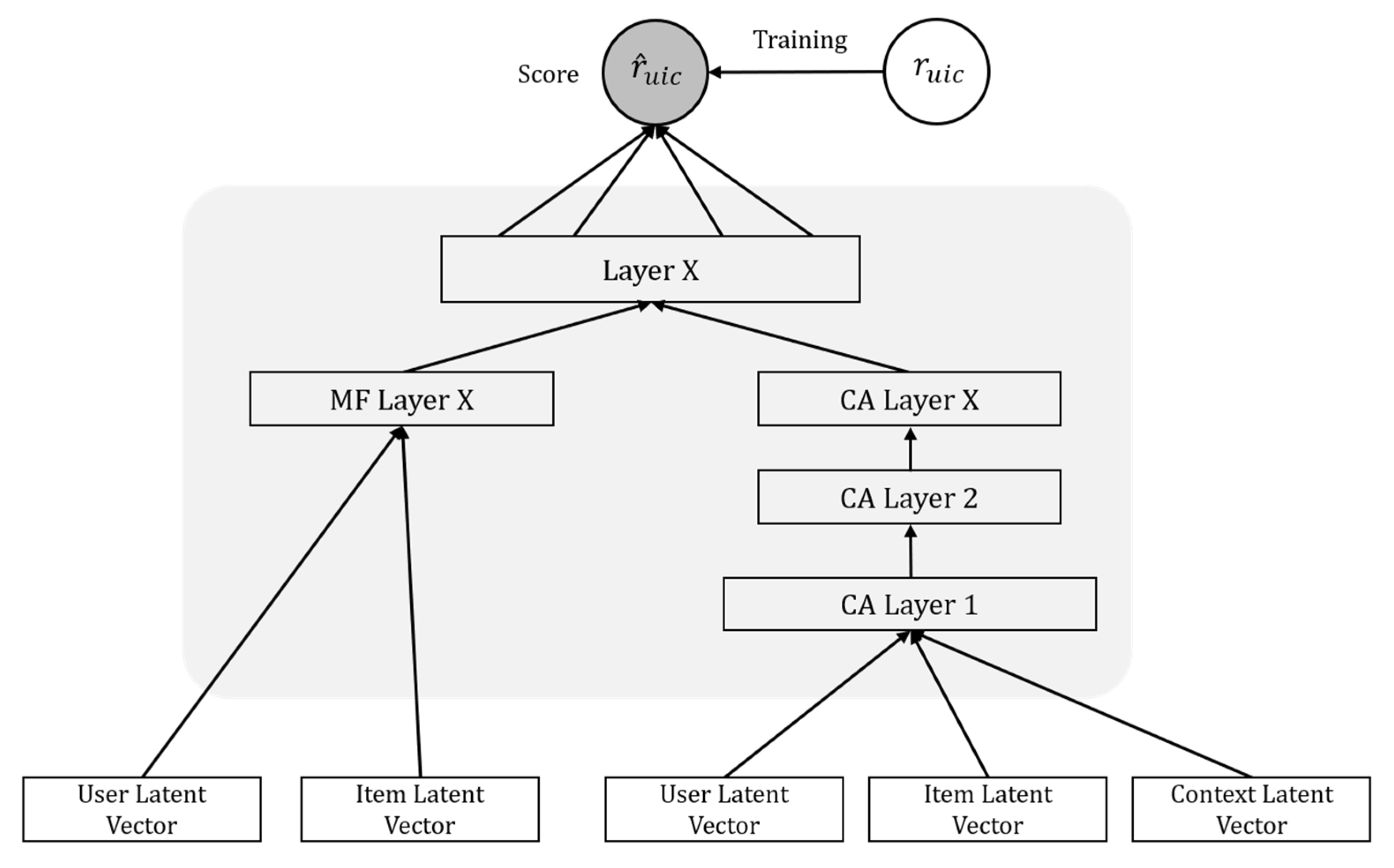
DRS (Dynamic Recommender System) refers to a recommender system that reflects changes in users or items over time. DRS predicts preferences by capturing time-varying data or temporal changes in various domains related to users or items. There are previous studies on DRS, and most of them have shown good performance in multimedia and e-commerce fields [20,21]. In the Netflix Prize held in 2009, Koren et al. proposed a study that considered user bias, item bias, and preference change and showed excellent performance [22]. Since then, there have been many studies on preference change. Ding et al. argued that users’ most recent item ratings are more likely to reflect their true preferences [23], so they proposed a weighting factor that reduces the similarity as the time difference increases. Chen et al. proposed a framework for a recommender system using tweet streams to take into account the rapidly changing user interests and topic popularity over time [24]. They studied how to provide users with topics of interest in a timely manner. Liu et al. proposed a dynamic model that considers preference changes for points of interest (POIs) in a given time period [25]. Jin et al. proposed a temporal model that captures multiple drifts using deep learning to incorporate user interest or item changes into preference prediction [26]. It has been shown that this approach performs well by tracking preference changes and can achieve better results than recommender systems that do not consider preference changes [27,28]. Among DRSs, TimeSVD++ is an extension of the SVD (Singular Value Decomposition) model that utilizes user and item bias over time to reflect trends in user activity or items [29]. TMF (Temporal Matrix Factorization) is a method that models the temporal dependence of users through transition matrices between consecutive time periods, assuming that users’ preferences change gradually [30]. BTMF (Bayesian Temporal Matrix Factorization) is an extension of TMF that extends MF to a fully Bayesian treatment by applying presets to the hyperparameters. TimeTrustSVD is an improved TrustSVD algorithm that considers the impact of time and trust relationships on users and items, and the impact of time on scores [31]. The proposed method aims to improve accuracy by applying DRS to context-aware recommender system by referring to the method of applying a preference transition matrix to MF.

3. Proposed Model

In this paper, we propose a context-aware recommender system using preference transition matrices to predict changing preferences over time. The proposed method applies preference transition matrices to MFs to capture preference changes. The model also incorporates users’ preferences for contexts using deep learning. Section 3.1 presents a model that takes preference changes into account, while Section 3.2 illustrates the integration process with a context-aware recommendation model.
The notation used in this paper is shown in Table 1 below.

3.1. Matrix Factorization to Account for Changing User Preferences

To identify patterns in temporal data, we use state transition matrices that can represent the time-varying changes embedded in the data. In this paper, the matrix generated to capture preference changes over a range of time t is called a preference transition matrix, where S i N × d × d is the preference of user i and d is the latent space.
Table 2 shows a typical preference matrix for a recommender system. The preference matrix R is of size i × j and consists of rows representing items and columns representing users. There are values in the matrix where r i , j represents i ’s preference for item j .
MF is a technique that decomposes a user-item matrix into a user latent matrix, U , and an item latent matrix, V . The product of the user latent matrix and the item latent matrix is trained to resemble the values in the preference matrix. The matrices U and V are obtained by training the product of the user latent matrix and the item latent matrix to be similar to the values in the preference matrix. Finally, the predicted value of R is multiplied by the matrices U and V that are most similar to R, and R is the matrix filled with all the values in the matrix. In this way, MF can predict preferences that have not been evaluated by the user. The mathematical representation of MF is shown in Equation (1), and in this paper, we follow Non-Negative Matrix Factorization (NMF).
R i , j = U V   U 0 ,   V 0
The preference transition matrix S i is used to capture the change in preference of user i from the previous time ( t 1 ) to the next time ( t ) . Suppose S i exists with a latent space of 2, and S i is a unit matrix of the form [ 1 0 0 1 ] . It is characterized that multiplying any matrix by a unit matrix always results in a multiplicative matrix. Therefore, the implication that S i is a unit matrix is that there is no change in the user’s preferences. In another example, if S i is a matrix of the form [ 1.5 0 0 1 ] , we can say that preferences are shifting by the first factor.
R t = U t V t
R t 1 = U t 1 V t 1
R t T = U t T V t T
Figure 3 illustrates the Matrix Factorization method with a preference transition matrix. If we split the data into t non-overlapping time periods and apply MF, we get the following result.
Between each time period, there is a preference transition matrix ( S i N × d × d ) that reflects the change in preferences. we express user i ’ s user latent factor ( U i , t ) at time t as a formula, it is equal to (5).
U t = S t U t 1
Traditional NMF assumes that the data and latent factors are static. However, this is not appropriate for datasets where preference changes occur continuously. Therefore, in this paper, we apply a method to model user preference changes in user latent spaces U t and U t 1 from the previous time to the next time by using the preference transition matrix S t . By reflecting Equation (5) in Equation (2), the formula to obtain the preference of user i at time t using the user factor is as follows.
R t = U t 1 S t V t
If we assume T = 3, the data is split into R t , R t 1 , R t 2 . The loss function for this is as follows.
min U t , V t R t U t V t F 2
min U 1 t , V t 1 R t 1 U t 1 V t 1 F 2
min U t 2 , V t 2 R t 2 U t 2 V t 2 F 2
U t , V t , U t 1 , V t 1 , U t 2 , V t 2 0
· F 2 stands for the Frobenius norm. It shows how the process of previous times is reflected to get the preference for the current time t. Here is how Equation (7) reflects the preference transition matrix to capture the change in user preferences using Equation (5).
min U t 1 , s t , V t R t U t 1 S t V t F 2
min U 1 t , V t 1 R t U t 2 S t 1 V t 1 F 2
min U t 2 , V t 2 R t U t 2 V t 2 F 2
The preference transition matrix is learned as the change in preference over time between the latent user vectors. To account for user preference changes, we can use Equations (10)–(12) to represent the following objective function.
L = min U t , s t , V t t = 1 T R t U t V t F 2
+ t = 2 T U t S t U t 1 F 2
+ λ 1 ( U t 1 + V t 1 + S t 1
+ λ 2 n = 1 N S t 1 I F 2
where I d × d is a unit matrix and · 1 denotes l 1 -norm. The third term is the l 1 -norm regularization, which makes the factor matrix U t , V t , S t   a sparse matrix. The parameter λ 1 controls the effect of the λ 1 -norm normalization. The fourth term represents the temporal normalization between the user preference matrices. The parameter λ 2 controls how biased we want the model to be toward past interests/attributes. The objective function is shown to compute the change in user interest over time T .

3.2. Context-Aware Recommender System Considering Change in Preference

Context-aware recommender systems need to model the relationship between users, items, and contexts. The problem of data sparsity is much more serious for context-aware recommender systems than for recommender systems using only users and items. If the contextual information is applied to the previous method using the transition matrix, the pattern of the data will be blurred. Therefore, in this paper, we chose a method to integrate with a context-aware recommender system that considers data sparsity. The framework of the proposed method is as follows.
Figure 4 is a combination of an autoencoder and a neural network. The input consists of several feature vectors. There is an autoencoder whose input and output are user vector, item vector, and context vector, and a neural network that is trained by targeting the score from the middle hidden layer. When a dataset has n(x, y) pairs, x is a data record containing user, item, and context information, and y is labeled with the score evaluated by the user. Each field in x is represented as a binary vector with one-hot encoding. In Figure 4, y u i c denotes the actual score that user u rated item i in context c , and y ^ u i c denotes the predicted score.
y ^ u i c = σ ( w x k / 2 + b )
If the total number of layers is k , then y ^ u i c can be obtained from layer k / 2 . To train the proposed model, we need to go through two processes. First, v u , v i , v c in the output of Figure 3 should minimize the loss with respect to v u , v i , v c in the input. Here, context is separated into context dimension and input. The expression is equivalent to (15).
L A E = min θ   v V X X 2 + α l ( w A E 2 + b A E 2 )
X means the entire input, and the output of the autoencoder given the input X is X . We applied Exponential Linear Units (ELU) to learn while reducing the error of X and X . Regularization terms are added to prevent overfitting. Autoencoders are mainly used to reduce the dimensionality of input data or to extract features from input data. In Figure 5, the hidden layer represents context representations when the input is context. Using the context representation obtained from Equation (15), y ^ u i c is obtained. y ^ u i c is trained to minimize the loss between it and y ^ u i c . This is expressed in the following Equation (16).
L N N = min θ y Y ( y u i c y ^ u i c ) 2 + β l ( w N N 2 + b N N 2 )
Equations (15) and (16) are trained simultaneously. To train the proposal method, we apply Adaptive Moment Estimation (Adam). Adam is a popular optimization technique.
In Figure 5, the MF layer represents the model that considers preference changes in Section 3.1, and the CA layer represents the context-aware recommendation model in Section 3.2. The details of each model are described above. The output from each model is concatenated to get the final prediction.

4. Experiments

4.1. Data Sets

For the experiments of the proposed method, we used two datasets. We used a dataset of real users to check whether the performance improves when considering the preference changes assumed in this paper. The detailed dataset information is shown in Table 3.
-
The University Cafeteria dataset is from a food court at Chungnam National University, Korea. To distinguish individual users, they were identified by their encrypted credit card numbers. There are four contextual dimensions: time, day, weather, and temperature. Time of day has three contextual conditions: Breakfast, Lunch, and Dinner. Day of the week has 6 contextual conditions: Mon, Tue, Wed, Thu, Fri, Sat. Weather has 3 contextual conditions: Sunny, Rain, Snow. Temperature has 4 contextual conditions: Hot, Warm, Cool, Cold.
-
The Instacart dataset is from Instacart, an online-based fresh food delivery service in the United States. It has user_id, which identifies the user, and order_id, which is the order number. The order_id can be thought of as the identification number of a shopping cart that contains multiple items. There are about 30 million rows of order_product, which is the product in the order_id. The Instacart dataset has the day of purchase, time of purchase, and time since purchase, but we don’t know the exact date of purchase, so we assigned the first purchase date as January. There are three contextual dimensions: day of the week, time of day, and weekday/weekend.
We used 5-fold cross validation, with 80% of users as training set and 20% as test set.

4.2. Evaluation Measures

There are many types of performance evaluation measures for recommender systems. There are RMSE (Root Mean Square Error) and MAE (Mean Average Error) to measure the error of the predicted score. Precision and Recall are methods that recommend based on the degree of preference rather than score. Although the dataset is represented as a score instead of preferred/dispreferred, the actual recommender system does not show the score to the user. Therefore, it recommends items in the order of the highest score based on the predicted score, and uses Precision and MAP (Mean Average Precision) to measure the performance based on the order. Precision@N is equal to Equation (17).
Precision @ N = | { r e l e v a n t   i t e m s } { t o p N   i t e m s } | N
Precision is the percentage of recommended items that the user is interested in. Given a list of recommended items for a <User, Context> pair, we measure the hit ratio.
When a recommender system recommends items, it’s very important which items appear at the top. However, the Precision measure does not consider the order. We use MAP as an accuracy measure that considers the order of items. Before we can find MAP, we need to find AP (Average Precision). AP@N can be found through Equation (18).
AP @ N = 1 m k = 1 N ( P ( k )     i f   k t h   i t e m   w a s   r e l e v a n t )
= 1 m k = 1 N P ( k ) · r e l ( k )
r e l ( k ) =   { 1 ,                 i f   r e l e v a n t 0 ,                   o t h e r w i s e
In the above expression, m is the number of relevant items, and P(k) is the precision up to index k. rel(k) has a value of 1 or 0 depending on whether the item was relevant. The accuracy of the recommendation for one user is AP, and the accuracy for all users U is MAP. MAP@N can be obtained through Equation (19). In the experiments in this paper, N is set to 10.
MAP @ N = 1 | U | u = 1 | U | ( A P @ N ) u
Precision and MAP consider higher values to be better performance.

4.3. Compared Methods

To measure the performance of the proposed method, we selected and compared each model in Non-contextual RS, Context-Aware RS, and DRS. Among the non-contextual algorithms, we selected User KNN, SVD++, PMF, and FM. Among the context-aware recommender systems, CAMF, ItemSplitting, and CSLIM were selected for comparison. Among DRS, we compared the performance with TimeSVD, TMF, BTMF, and TimeTrustSVD.
The proposed method requires some parameters to be set. Each parameter value is selected through experiments. First, we set the latent factor to 100 and the learning rate to 0.001. The regularization parameters in Equation (13) are set to λ 1 = 0.001 and λ 2 = 0.01 . In Equations (15) and (16), we set α = 0.01 and β = 0.001 , respectively. The learning rate of PMF was set to 0.001. The learning rate for TimeSVD++, TMF, BTMF, and TimeTrustSVD was set to 0.003. In addition, TMF and BTMF set the factor to 20 based on other studies, and the number of factors for other latent factor-based models was set to 100.

4.4. Results of the Experiments

In this paper, we proposed a model to improve accuracy by reflecting preference changes over time in context-aware recommender systems. Therefore, we compared the performance of the proposed model with representative RS, CARS, and DRS to check whether the accuracy is improved by considering preference changes.
First, the Precision results were examined by the DRS over different periods, and the results are shown in Figure 6. For the experiment, we set the time period to 1 month, 3 months, 6 months, and 12 months. One month was too small a number of data to identify patterns in the data, so we set the time period to six months, which showed some performance. When we split the data into small chunks of time, the accuracy was low due to data sparsity. However, we can see that the performance gradually improves as we capture preference changes from long-term data.
The following table shows the experimental results of the baseline and proposed methods on the university cafeteria and Instacart datasets. Table 4 shows the Precision@N results for each model, and Table 5 shows the MAP@N results for each model.
The RSs include userKNN, SVD++, PMF, and FM. We set userKNN to 10 and the number of factors for the other methods to 100. In the University cafeteria dataset, userKNN and PMF showed good performance among RS, and we can see that the proposed method and PMF differed in precision by about 0.05 when N is 10. In RS, userKNN was the highest in terms of MAP, but it was about 0.08 lower than the proposed method. In the Instacart dataset, we can see that the proposed method performs slightly better than the University cafeteria, although the difference is not significant. This is likely due to the fact that it utilizes other additional information from the user to predict their preferences.
We compared CAMF, ItemSplitting, CSLIM, and the proposed method with the CARS model. In CARS, ItemSplitting generally performed well, but it has the disadvantage that it takes a lot of time because ItemSplitting measures the correlation between contexts and converts Item to Item+context, making the matrix two-dimensional. The better performance of the proposed method shows that it is effective in considering preference changes. Also, when comparing the two datasets, Instacart has a slightly smaller number of contextual dimensions and contextual conditions. We expected Instacart to be more accurate because CARS often has too much contextual information, which can lead to poor performance. However, the experimental results showed that the University cafeteria generally performed better. These results show that having the right amount of contextual information to influence preferences can improve performance.
Finally, we compared the precision and MAP of DRS and the proposed method. We compared the performance of TimeSVD, TMF, BTMF, TimeTrustSVD, and the proposed method as DRS models. Among the DRSs, BTMF has the highest precision and MA0P. It also has the smallest performance difference with the proposed method among the compared models. In general, DRS performed better than CARS, which suggests that the method that considers preference changes is better than the method that considers contextual information.

5. Conclusions and Future Work

In order to provide users with satisfactory recommendations, recommender systems utilizing additional information have been developed. Among them, context-aware recommender systems are based on the assumption that users’ preferences differ depending on the context in which they are placed. Context refers to the attributes that can influence a user’s preferences. However, a user will not always choose the same items in the same context. No one eats the same food every time it rains. In this way, users may change their preferences for personal reasons or due to trends.
Therefore, in this paper, we propose a context-aware recommender system that considers user preference changes over time. The proposed method is a context-aware recommender system model using a preference transition matrix to detect preference change and apply it to predict preference. For the experiments, we compared a recommender system that does not use contextual information with a context-aware recommender system and a recommender system that considers time. The experimental results showed that the additional information was generally better than the existing recommender system. When comparing the comparison model and Precision, the proposal method showed better results. According to the MAP, BTMF showed the smallest difference, indicating that the method that considers preference changes generally has good accuracy. Based on this, we expect to be able to provide improved recommendations to long-term users through the suggested method.
The proposed method incorporates the division of data into time units to account for temporality. However, during this process, it was observed that splitting the data into weekly and monthly time units resulted in low accuracy due to data sparsity. This indicates that while the model effectively captures long-term time preference changes compared to other models, it struggles to capture short-term preference changes. Therefore, additional research is required to explore methods for effectively capturing short-term preference changes.

Author Contributions

Conceptualization, S.-Y.J. and Y.-K.K.; methodology, S.-Y.J.; investigation, S.-Y.J.; validation S.-Y.J. and Y.-K.K.; writing—review and editing, S.-Y.J.; supervision Y.-K.K. All authors have read and agreed to the published version of the manuscript.

Funding

This work was partly supported by Institute of Information & communications Technology Planning & Evaluation (IITP) grant funded by the Korea government (MSIT) (No. RS-2022-00155857, Artificial Intelligence Convergence Innovation Human Resources Development (Chungnam National University)) and the MSIT (Ministry of Science and ICT), Korea, under the Innovative Human Resource Development for Local Intellectualization support program (IITP-2023-RS-2022-00156334) supervised by the IITP (Institute for Information & communications Technology Planning & Evaluation).

Data Availability Statement

Data Availability Statement: Publicly available datasets were analyzed in this study. This data can be found here: https://www.kaggle.com/c/instacart-market-basket-analysis accessed on 31 July 2021.

Conflicts of Interest

The authors declare no conflict of interest.

References

  1. Zhang, S.; Yao, L.; Sun, A.; Tay, Y. Deep learning based recommender system: A survey and new perspectives. ACM Comput. Surv. (CSUR) 2019, 52, 1–38. [Google Scholar] [CrossRef]
  2. Chen, J.; Dong, H.; Wang, X.; Feng, F.; Wang, M.; He, X. Bias and debias in recommender system: A survey and future directions. ACM Trans. Inf. Syst. 2023, 41, 1–39. [Google Scholar] [CrossRef]
  3. Zheng, X.; Zhao, G.; Zhu, L.; Zhu, J.; Qian, X. What you like, what I am: Online dating recommendation via matching individual preferences with features. IEEE Trans. Knowl. Data Eng. 2022, 35, 5400–5412. [Google Scholar] [CrossRef]
  4. Aggarwal, C.C. Recommender Systems; Springer International Publishing: Berlin/Heidelberg, Germany, 2016. [Google Scholar] [CrossRef]
  5. Sarker, I.H. Context-aware rule learning from smartphone data: Survey, challenges and future directions. J. Big Data 2019, 6, 1–25. [Google Scholar] [CrossRef]
  6. Casillo, M.; Gupta, B.B.; Lombardi, M.; Lorusso, A.; Santaniello, D.; Valentino, C. Context aware recommender systems: A novel approach based on matrix factorization and contextual bias. Electronics 2022, 11, 1003. [Google Scholar] [CrossRef]
  7. Batmaz, Z.; Yurekli, A.; Bilge, A.; Kaleli, C. A review on deep learning for recommender systems: Challenges and remedies. Artif. Intell. Rev. 2019, 52, 1–37. [Google Scholar] [CrossRef]
  8. Zhao, G.; Liu, Z.; Chao, Y.; Qian, X. CAPER: Context-aware personalized emoji recommendation. IEEE Trans. Knowl. Data Eng. 2020, 33, 3160–3172. [Google Scholar] [CrossRef]
  9. Kalloori, S.; Chalumattu, R.; Yang, F.; Klingler, S.; Gross, M. Towards Recommender Systems in Augmented Reality for Tourism. Inf. Commun. Technol. Tour. 2023, 2023, 267–272. [Google Scholar]
  10. Zheng, Y.; Mobasher, B.; Burke, R.D. Incorporating Context Correlation into Context-Aware Matrix Factorization. In Proceedings of the 2015 International Conference on Constraints and Preferences for Configuration and Recommendation and Intelligent Techniques for Web Personalization, Buenos Aires, Argentina, 25–27 July 2015; Volume 1440. [Google Scholar]
  11. Suhaim, A.B.; Berri, J. Context-aware recommender systems for social networks: Review, challenges and opportunities. IEEE Access 2021, 9, 57440–57463. [Google Scholar] [CrossRef]
  12. Baltrunas, L.; Ludwig, B.; Ricci, F. Matrix factorization techniques for context aware recommendation. In Proceedings of the Fifth ACM Conference on Recommender Systems, Chicago, IL, USA, 23–27 October 2011; pp. 301–304. [Google Scholar] [CrossRef]
  13. Baltrunas, L.; Ricci, F. Experimental evaluation of context-dependent collaborative filtering using item splitting. User Model. User-Adapt. Interact. 2014, 24, 7–34. [Google Scholar] [CrossRef]
  14. Zheng, Y.; Mobasher, B.; Burke, R. CSLIM: Contextual SLIM recommendation algorithms. In Proceedings of the 8th ACM Conference on Recommender Systems; 2014; pp. 301–304. [Google Scholar]
  15. Jeong, S.Y.; Kim, Y.K. Deep learning-based context-aware recommender system considering contextual features. Appl. Sci. 2022, 12, 45. [Google Scholar] [CrossRef]
  16. Livne, A.; Unger, M.; Shapira, B.; Rokach, L. Deep context-aware recommender system utilizing sequential latent context. arXiv 2019, arXiv:1909.03999. [Google Scholar] [CrossRef]
  17. Mohamed, S.A.E.M.; Soliman, T.H.A.; Sewisy, A.A. A context-aware recommender system for personalized places in mobile applications. Int. J. Adv. Comput. Sci. Appl. 2016, 7, 442–448. [Google Scholar]
  18. Bahramian, Z.; Abbaspour, R.A.; Claramunt, C. A Context-Aware Tourism Recommender System Based on a Spreading Activation Method. International Archives of the Photogrammetry. Remote Sens. Spat. Inf. Sci. 2017, 42, 333–339. [Google Scholar] [CrossRef]
  19. Achmad, K.A.; Nugroho, L.E.; Djunaedi, A. Tourism contextual information for recommender system. In Proceedings of the 2017 7th International Annual Engineering Seminar (InAES), Yogyakarta, Indonesia, 1–2 August 2017; pp. 1–6. [Google Scholar] [CrossRef]
  20. Rana, C.; Jain, S.K. A study of the dynamic features of recommender systems. Artif. Intell. Rev. 2018, 43, 141–153. [Google Scholar] [CrossRef]
  21. Lopes, P.; Roy, B. Dynamic recommendation system using web usage mining for e-commerce users. Procedia Comput. Sci. 2015, 45, 60–69. [Google Scholar] [CrossRef]
  22. Koren, Y.; Bell, R.; Volinsky, C. Matrix factorization techniques for recommender systems. Computer 2009, 42, 30–37. [Google Scholar] [CrossRef]
  23. Ding, Y.; Li, X. Time weight collaborative filtering. In Proceedings of the 14th ACM International Conference on Information and Knowledge Management, Birmingham, UK, 21–25 October 2005; pp. 485–492. [Google Scholar]
  24. Chen, C.; Yin, H.; Yao, J.; Cui, B. Terec: A temporal recommender system over tweet stream. Proc. VLDB Endow. 2013, 6, 1254–1257. [Google Scholar] [CrossRef]
  25. Liu, Y.; Liu, C.; Liu, B.; Qu, M.; Xiong, H. Unified point-of-interest recommendation with temporal interval assessment. In Proceedings of the 22nd ACM SIGKDD International Conference on Knowledge Discovery and Data Mining, San Francisco, CA, USA, 13–17 August 2016; pp. 1015–1024. [Google Scholar] [CrossRef]
  26. Jin, Z.; Zhang, Y.; Mu, W.; Wang, W.; Jin, H. Leveraging the dynamic changes from items to improve recommendation. In Conceptual Modeling: 37th International Conference, ER 2018, Xi'an, China, 25–28 October 2018; Springer: Cham, Switzerland, 2018; pp. 507–520. [Google Scholar]
  27. Lin, K.; Liu, D. Category-based dynamic recommendations adaptive to user interest drifts. In Proceedings of the 2014 Sixth International Conference on Wireless Communications and Signal Processing (WCSP), Hefei, China, 23–25 October 2014; pp. 1–6. [Google Scholar] [CrossRef]
  28. Wangwatcharakul, C.; Wongthanavasu, S. Dynamic collaborative filtering based on user preference drift and topic evolution. IEEE Access 2020, 8, 86433–86447. [Google Scholar] [CrossRef]
  29. Koren, Y. Collaborative filtering with temporal dynamics. In Proceedings of the 15th ACM SIGKDD International Conference on Knowledge Discovery and Data Mining, Paris, France, 28 June–1 July 2009; pp. 447–456. [Google Scholar] [CrossRef]
  30. Zhang, C.; Wang, K.; Yu, H.; Sun, J.; Lim, E.P. Latent factor transition for dynamic collaborative filtering. In Proceedings of the 2014 SIAM International Conference on Data Mining, Philadelphia, PA, USA, 24–26 April; 2014; pp. 452–460. [Google Scholar] [CrossRef]
  31. Tong, C.; Qi, J.; Lian, Y.; Niu, J.; Rodrigues, J.J. TimeTrustSVD: A collaborative filtering model integrating time, trust and rating information. Future Gener. Comput. Syst. 2019, 93, 933–941. [Google Scholar] [CrossRef]
Figure 1. Input data when using time as a feature.
Electronics 12 02337 g001
Figure 2. Input data when using time in a sequential sense.
Electronics 12 02337 g002
Figure 3. MF process with preference transition matrices.
Electronics 12 02337 g003
Figure 4. Neural Context-Aware Recommender System.
Electronics 12 02337 g004
Figure 5. Illustration of the proposed model based on NCARS.
Electronics 12 02337 g005
Figure 6. DRS Precision@10 on University cafeteria datasets.
Electronics 12 02337 g006
Table 1. Notations.
Table 1. Notations.
NotationDescription
i , j Number of users, number of items
k Number of latent factors
R t     i × j Preference matrix at current time t
R t 1     i × j Preference matrix at time t − 1
R ^ i j t Time t user i item j preference prediction matrix
T Entire period
U i t     i × k User latent matrix at time t
U i t 1     i × j User latent matrix at time t − 1
V j t     k × j Item latent matrix at time t
W Time weights
λ 1 ,   λ 2 Normalization parameters
Table 2. Preference matrix for a recommender system.
V 1 V 2 V j
U 1 r 1 , 1 r 1 , 2 r 1 , j
U 2 r 2 , 1 r 2 , 2
U i r i , 1 r i , 2 r i , j
Table 3. Data sets.
Table 3. Data sets.
University CafeteriaInstacart
# of users37,289206,209
# of items9749,688
# of orders725,4383,421,083
Contextual Dimensions43
Contextual Conditions1613
Sparsity99.89%99.99%
Table 4. Compare Precision@N for each model.
DatasetUniversity CafeteriaInstacart
MethodN = 10N = 20N = 10N = 20
RSUserKNN0.0437320.0403580.0236720.035216
SVD++0.0085990.0110440.0473960.050524
PMF0.0622620.0688340.0507910.052613
FM0.0173690.0195940.0197620.028647
CARSCAMF0.0658360.0756250.0186420.022677
ItemSplitting0.0684980.0662350.0416530.040589
CSLIM0.0128350.0196620.0384520.037446
DRSTimeSVD0.0572900.0612110.0296480.029273
TMF0.0645220.0665070.0524730.052981
BTMF0.0776520.0809170.0645200.069118
TimeTrustSVD0.0638610.0641850.0349130.035499
Proposed method0.1148650.1075620.0851160.080427
Table 5. Compare MAP@N for each model.
DatasetUniversity CafeteriaInstacart
MethodN = 10N = 20N = 10N = 20
RSUserKNN0.1364820.1386230.0200440.022758
SVD++0.0823660.0804750.0954270.075211
PMF0.1076940.1084620.1724360.153776
FM0.0882190.0903250.0536410.058962
CARSCAMF0.0849630.0875810.0716280.070493
ItemSplitting0.1305310.0358160.1622850.158174
CSLIM0.0358160.0437460.0492640.050723
DRSTimeSVD0.0841900.0869970.0823580.085279
TMF0.1275220.1324900.1640150.170294
BTMF0.1786200.1712360.1702930.169470
TimeTrustSVD0.1072230.1149180.1475260.150711
Proposed method0.2236740.2026380.1975630.188249
Disclaimer/Publisher’s Note: The statements, opinions and data contained in all publications are solely those of the individual author(s) and contributor(s) and not of MDPI and/or the editor(s). MDPI and/or the editor(s) disclaim responsibility for any injury to people or property resulting from any ideas, methods, instructions or products referred to in the content.

