Efficient Multiclass Classification Using Feature Selection in High-Dimensional Datasets

Abstract

Feature selection has become essential in classification problems with numerous features. This process involves removing redundant, noisy, and negatively impacting features from the dataset to enhance the classifier’s performance. Some features are less useful than others or do not correlate with the system’s evaluation, and their removal does not affect the system’s performance. In most cases, removing features with a monotonically decreasing impact on the system’s performance increases accuracy. Therefore, this research aims to propose a dimensionality reduction method using a feature selection technique to enhance accuracy. This paper proposes a novel feature-selection approach that combines filter and wrapper techniques to select optimal features using Mutual Information with the Sequential Forward Method and 10-fold cross-validation. Results show that the proposed algorithm can reduce features by more than 75% in datasets with large features and achieve a maximum accuracy of 97%. The algorithm outperforms or performs similarly to existing ones. The proposed algorithm could be a better option for classification problems with minimized features.

1. Introduction

Feature selection is used as a dimensionality reduction technique in most of the problems of different research areas, where many attributes are available due to improved data collection methods [1,2,3,4]. For defining a single sample, a large set of features increases the computational complexity and the manifold space dimension. Out of these many features, most of the features are not informative or sometimes misleading, thus degrading the classifier’s performance. In many other works, datasets are presented with missing values [5,6]. The strategies used for selecting features aim to find the optimal subset of features and discard redundant information. Methods for the selection of optimal features, which are exhaustive, are NP-hard. So, in order to perform these tasks, intelligent frameworks are designed. According to their working principle, these frameworks are divided into filter, wrapper, and embedded methods [7]. Filter methods use intrinsic properties of data to evaluate the features and are efficient and computationally faster. Wrapper methods evaluate the features at the time of the learning mechanism. These are more accurate than the filter methods. However, these methods sometimes cause overfitting. The overfitting could be overcome by using different techniques such as the hold-out method, cross-validation, L1/L2 regularization, etc. Embedded methods try to use the strength of these two methods. These methods are computationally costlier than filter methods and are not smart with respect to handling high-dimensional data. Classification problems are those that are used to identify which new data belong to which known class. Classification could be classified into two types: (a) binary classification and (b) multi-classification. In binary classification, there are two output classes in total; i.e., the output could be either yes or no; for example, in the case of cancer, a person has cancer or does not. In multi-classification for the problem, the output comes in k classes, where k is an integer ranging from 2 to n. Depending on the output, the classification problem could be linearly separable or linearly inseparable. Multiple methods have been devised to solve these problems. Some of them include K-Nearest Neighbor [8], Random Forest [9], Gradient Boosting [10], SVM [11], and Ada Boost [12].

The methods designed for feature selection are used in dealing with many challenges such as reducing the data dimensionality, computational complexity, computational cost, or storage space, or increasing the classification rate, and the ratio of features selected [13,14]. A method designed for feature selection cannot cover all the existing challenges in one go. So most of the existing methods deal with only accuracy. In existing methods, data with fewer features have average accuracy. Increasing the number of features (high-dimensional dataset), the accuracy abruptly decreases. Moreover, most of the existing challenges, such as computational cost, storage space, ratios of features selected, and high classification rate with fewer features, are not covered by previous work, and they remain challenges for today also.

Therefore, concerning the previous work and existing challenges, we have proposed a hybrid algorithm. Through this algorithm, we try to overcome the issues not handled with optimality in previous work and some of the existing challenges. The proposed hybrid algorithm combines filter and wrapper techniques to select optimal features using Mutual Information with a Sequential Forward Selection method (a greedy method) abbreviated MISFS for feature selection and calculating classification accuracy of multiclass datasets. The algorithm in the first phase applied the Mutual Information method on the dataset to remove those features which are highly independent compared to the target. After removing those features, in the second phase, we applied the Sequential Forward Feature Selection method on the remaining features to select the best features having optimized accuracy. Selecting filter methods in the first phase involves less computational time. By taking Mutual Information as a filter approach, redundant data are easily removed. Moreover, with this method, one can determine how relevant the target class is to the input features and also how relevant individual features are to each other. Selecting the Sequential Forward Selection method in the second phase as a wrapper approach involves less computational time and is robust against overfitting. The proposed algorithm MISFS covers a few existing challenges, such as maximum reduction of features in high-dimensional datasets, higher classification rate, and less computational time, with the limitation of not addressing the computational space and other complexities.

The paper is framed with Section 2 covering the background regarding dimensionality reduction and different feature-selection models available in the literature. Section 3 discusses the related work on the different methods of selecting features and classification problems with accuracy available in the literature. Section 4 covers the methodology of the novel feature-selection approach MISFS with the algorithm. Section 5 presents the experimental evaluation of the proposed methodology on different problems. This section covers the experimental setup with details of the datasets covered, performance metrics used for measuring performance, comparison techniques used to include results, and discussion on different datasets with their performance evaluation and comparisons with other multiple techniques and the other research work. Section 6 covers the conclusion, which includes the algorithm’s performance and future work.

2. Background

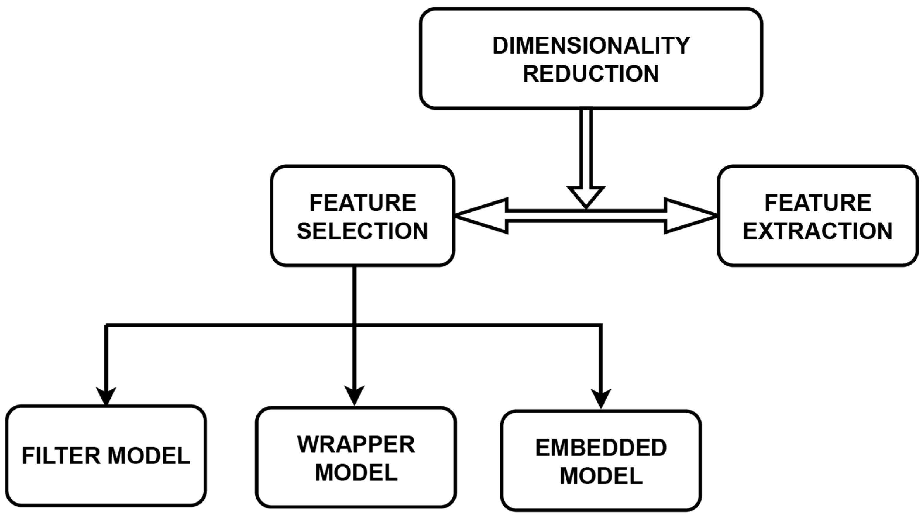
2.1. Dimensionality Reduction

When we have selected the dataset for work, we have no idea about which features are essential concerning dependent features, which are noisy, irrelevant, or redundant. Most of the real-life application areas include bioinformatics, speech recognition, the oil industry, text processing, the Internet, engineering applications, medicine, diseases, and many more. The datasets covered in these areas are high-dimensional data with noisy, irrelevant, and redundant attributes. Thus, the feature-selection process is applied to selecting those attributes that result [7] in minimum computing time with high accuracy. Achieving these results includes numerous factors, such as:

• Is there any methodology to find the optimal features?
• Is there any evaluation process that could determine that the selected features are optimal?
• Is there a methodology used for independent feature-selection applications?

Other motivations for performing feature selection or dimensionality reduction are to perform general data reduction (minimum storage space with minimum execution time), feature set reduction (to save resources for the next step of data collection or utilization), performance improvement, and higher data understanding.

Figure 1 presents the dimensionality reduction.

From paper [7], the general framework of the feature-selection process, shown in Figure 2, could be categorized as follows:

• In the first step, generate the feature subset by applying some methodology.
• After that, evaluate the feature subset.
• Then the termination conditions are applied.
• Finally, the result is validated.

2.2. Model for Feature Selection

A different feature-selection model includes a filter, wrapper, and embedded models [7]. Filter-based feature-selection methods select the features using several scoring metrics in an unsupervised fashion, requiring no classifier in its core. Compared to the other two methods, they are computationally more efficient. However, in terms of performance, wrapper methods are far better than filter methods. Wrapper methods select the optimal feature set by applying the learning algorithm at its core. The heart of this method is the classifier, whose purpose is to upsurge the performance of carefully chosen features at each iteration. The computational cost of the wrapper method is greater compared to filter methods. Filter and wrapper methods differ mostly by evaluation criteria. Filter methods are sometimes acclimatized with feature-ranking methods. Similar to wrapper methods are embedded methods, using the inherent properties of the model as a metric during the learning phase. The more complex problems are handled easily via embedded methods in contrast with filter methods. Moreover, in the case of larger training samples, embedded methods beat the filter methods. Hybrid methods also exist, which are a combination of filter and wrapper methods first applying the filter method to rank features to generate a nested subset of features; these are computed via a learning mechanism, i.e., a wrapper approach.

Algorithms designed based on these methods are not perfect or suitable for all real-life applications. Selecting an algorithm suitable for a given application area or all application areas is a tedious and complex task. The reason for this is that each application area is different from others. Moreover, the model or algorithms designed to solve a problem in a particular domain work differently depending on the data available. A small change in data could lead to different feature selections. So, the algorithm designed to solve a problem in one domain does not work well in another domain. Furthermore, each model could handle some of the challenges mentioned above. Most of the models available in the literature deal either with accuracy or reduction in features. However, achieving both at the same time is not achieved at a higher rate with these algorithms.

So, the purpose of this proposed methodology is to handle most of the challenges. It can be seen that the MISFS method achieves higher accuracy with maximum feature reduction on both low- and high-dimensional datasets. Moreover, the computational efficiency is low compared to existing methods, reduced data dimensionality is achieved, and the ratio of features selected is also calculated. This approach’s limitation is that it covers storage space to a very limited extent.

3. Related Work

The ability to acquire massive data in an existing period is a two-edged sword. Firstly, it allows us to analyze features more soundly due to the availability of more information about data. On the other hand, storing and processing these data is becoming more complex. Thus, techniques needed for dimensionality reduction are becoming more important because they help to remove features that are less needed without impairing the learner’s performance. Features that cannot discriminate the samples from different classes or clusters are irrelevant. The learning performance of the system is not hampered after removing such features. However, most of the time, the system’s performance is improved if a suitable model is used for performing feature selection depending on the area and type of problem selected.

Most of the research has been carried out, and many overview papers have been designed, to evaluate feature-selection methods available in the literature [1,7] in detail with their categorization. There are major studies in the area of classification problems, which include both binary and multi-class problems. Filter methods are used for counting the number of samples misclassified in two gene expression datasets [15]. Classification accuracy is calculated for artificial datasets [16] using different filters, wrappers, and embedded methods. Again, the microarray datasets are considered by [17] for calculating the classification accuracy using filter methods. Some reviewed the ensemble feature-selection techniques for classification [18]. In [19], the authors used various strategies, such as considering sentiment data for classification and using ensemble feature selection with hesitant fuzzy sets to attain results. They selected the top k features based on a relevancy score. The existing algorithms do not address all the existing challenges. Mostly, these methods cover only accuracy as a parameter. The weakness of these methods is that they do not cover the number of features selected, computational time, and storage space and are tuned via specific feature-selection methods and low accuracy in high-dimensional datasets.

In the case of diseases, there are common symptoms for some diseases. Therefore, diagnosing them is sometimes a little complex, so various optimization techniques are required to overcome this problem. Research has also been carried out on diseases caused by diabetes. The authors of [20] used the deep learning technique to predict eye, kidney, and cardiovascular diseases caused by diabetes. They used statistical methods to evaluate the performance. Most research has been carried out on the widely used the PIMA Indian Diabetes Dataset available at the UCI repository. One of the research works in [21] predicted diabetes by employing a classification model based on the Synthetic Minority Oversampling Technique and DT, thus improving the accuracy of the estimation of diabetes by eliminating class imbalance. They achieved a classification rate of 94.70% on the dataset considered. However, these existing research works have weaknesses in that they do not handle existing issues such as reduction in data dimensionality, computational cost, and higher classification accuracy but somehow achieved the accuracy at par level. Most reports on methods do not outline their weaknesses.

The authors of [22] implemented PCA and PSO for feature selection in multiple combinations with classification algorithms on the PIMA Indian Diabetes Dataset and the Localized Diabetes Dataset (LDD) gathered from Bombay Medical Hall, Upper Bazar, Ranchi, India, and achieved the highest classification rate of 79.56% with a combination of PCA and Logistic Regression for the PIMA Indian Diabetes Dataset and 95.58% for the LDD with PCA–PSO–C4.5 DT. This showed that the efficiency of the proposed model shows different performances on two datasets. However, it is better than the traditional approach in terms of increased accuracy, as mentioned in this paper. Moreover, there was a 50% reduction in features in both datasets via PCA and PSO. However, the authors remain silent on computation time and storage space and do not cover the high-dimensional data to evaluate the performance of the proposed method. Moreover, they do not guarantee that the same performance and the same percentage of reduction in features will be achieved on other datasets. A similar task was addressed by [23] while calculating the accuracy of the PIMA Indian Diabetes Dataset. They compared the performance of the Support Vector Machine, ANN, Naïve Bayesian, J48 DT, and Bagging methods and also added the performance of the Genetic Algorithm with Support Vector Machine. Moreover, they analyzed the weaknesses and strengths of these methods. They concluded that statistical methods are not successful on categorical data and handling missing values; that is why machine learning methods are used. In [24], they used the SOM optimization algorithm with four heuristic algorithms, namely Particle Swarm Intelligence (PSO), Newton-based self-organizing map PSO, self-organizing map Harmony Search Algorithm and self-organizing map Swarm. They implemented it on various bio-medical datasets. They compared the performance of these on the PIMA Indian Diabetes Dataset, Appendicitis, Heart, Hepatitis, Mammographic, Wisconsin Breast Cancer, and New Thyroid datasets. They achieved 91% accuracy on the New Thyroid dataset using the Newton-based self-organizing map PSO and 97% accuracy on the Wisconsin dataset through the self-organizing map Harmony Search Algorithm. The method exhibited a good quantization error for clustering and good accuracy with statistical measures. The authors proposed that multi-strategy SOM deep mapping learning can be adopted for multi-dimensional unstructured big-data problems. However, they have issues in dealing with big-data preprocessing.

Researchers have proposed various feature-selection methodologies designed with the Mutual Information (MI) technique. This is an approach based on the filter method. The first classification approach using MI dates back to [25]. In that study, the authors used a Mutual Information-based feature-selection method for text classification. The degree of correlation between the independent feature and dependent feature is calculated with Mutual Information and also helps in filtering out the irrelevant features. This method does not consider the relationship between the candidate and selected features. Moreover, in cases of heavily redundant data, the performance of Mutual Information is degraded. The issue of not considering the relationship between the candidate and selected features is considered in [26]. The authors of that study proposed Mutual Information based on Feature Selection (MIFS) which checks for the availability of unnecessary information between candidate features and the selected features.

The patient’s records are maintained through biomedical datasets containing multiple features. Several methods based on the wrapper and hybrid filter wrapper are used as ideal methods. Hybrid methods built on the Information Gain Genetic Algorithm [27] and Information Gain Particle Swarm Intelligence [28] showed the classification accuracy of combined filter and wrapper methods. In [27], the authors concluded that no classification technique outperforms all the other existing methods. They also concluded that the Genetic Algorithm somewhat improves the classification performance of different classifiers. The Artificial Bee Colony algorithm [29] used only seven features on the Cleveland Heart Disease dataset with a better classification accuracy compared to other feature-selection methods. Feature selection is carried out with Artificial Bee Colony methodology, and the performance is measured using the KNN classifier; the performance is excellent on the Cleveland Heart Disease dataset [30]. There are a few other domains in which LSTM networks have been successfully applied in sequence classification. For example, [31] used the LSTM network for air-quality prediction. The authors used data from air-quality sensors for the same purpose. They cleaned the raw data and filled in the missing data using edge-based components exploiting temporal and spatial information. The predicted accuracy was improved by 40.18% on the mean absolute percentage error.

This section on previous work shows that various feature-selection methods have been designed for classification problems on different diseases. Most of researchers used the methods to deal with classification accuracy, and some dealt with feature selection on different datasets and then calculated the accuracy. However, it is noteworthy that most of the methods do not provide higher accuracy with maximum feature reduction. Moreover, most of the existing challenges, explained above, are not handled with the existing methods. This research proposes a methodology, MISFS, which identifies the issues with the existing methods and tries to find solutions to most of the existing challenges. The proposed method uses the hybrid filter–wrapper method to cope with the issues mentioned in the literature. This combination benefits from the advantages of both the filter and wrapper methods, thus improving the classification accuracy; some of those advantages are reduced feature set, short computational time, and small storage space. Mutual Information (MI) is used as a filter method to rank the features and then select the features with higher ranking from all feature sets, passing the higher ranked features to Sequential Forward Feature Selection (SFS)—a greedy-based wrapper method—for further selection of features and calculating the accuracy. Thus, the maximum amount of features of lesser importance and redundant and noisy features are removed while achieving higher accuracy. As the approach is greedy-based, it decreases the computational complexity as a whole. Thus, the proposed MISFS method covers existing challenges regarding data dimensionality, computational complexity, computational cost, storage space to some extent, classification accuracy, and the ratio of features selected.

The proposed MISFS method covers the application area of the medical field but it could be used for different application areas.

4. Methodology

4.1. Overview of MISFS Approach

Here the authors have proposed an approach, MISFS, for selecting optimized features to obtain a good classification rate. We have designed a hybrid approach for selecting optimized features. Here, we utilized the strengths of both the filter and wrapper approaches by exploiting their diversified evaluation capabilities in both methodology phases. In this process, we used the strengths of filter and wrapper methods. The filter approach, which considers only the data for evaluation, is algorithm-independent. The wrapper approach considers both the data and the learning algorithm for evaluation and is algorithm-dependent. Separately, both have some disadvantages, which are overcome by the hybrid approach we propose.

4.2. Abstract View of MISFS and Comparison Methods

We propose a methodology called MISFS for feature selection and calculating accuracy. First of all, the dataset is divided into a training set and a test set. After that, MISFS is implemented on the training set to find the optimal features. After finding the optimal features, the training data accuracy and testing data accuracy are calculated using MISFS with KNN and LR. Then, the results of the MISFS are compared with three different styles:

• First, after calculating the accuracy of MISFS, we implemented different classifiers on the original dataset, calculated the classification rate, and compared the result with MISFS.
• Then, again, we implemented the Pearson Correlation method for feature selection, calculated the accuracy of the different threshold values, and compared the result with MISFS.
• Again, we compared the MISFS results with the prevailing work results.

Figure 3 shows an abstract view of the overall flow of calculation and comparison of results.

4.3. Implementation of MISFS

The MISFS approach, designed for feature selection, is a hybrid approach, as explained in Section 4.1, and is implemented in two phases. The first phase is called Phase 1, and the second phase is called Phase 2. Each phase can be summarized as follows:

(i.)

First phase: We implemented the filter approach, and in the second phase, we implemented the wrapper approach. The main task of the algorithm is to calculate the improved classification rate of the datasets after feature selection. So, in the first phase, we implemented Mutual Information, which is a filter method, for feature selection. Through this method, we selected features highly correlated with the output class. After that, by selecting these features, we implemented our second phase.

(ii.)

Second phase: We implemented the Sequential Forward Feature-Selection (SFS) method, a wrapper model, for feature selection. This methodology is based on the greedy approach. Here, the classifier first calculates the performance of each feature individually. After that, in the next step, it selects the feature with the best performance, pairs it with the remaining features, and evaluates the classifier’s performance. For clarification, let us say there are four features f₁, f₂, f₃, and f4. In the first step, the individual performance of each feature is evaluated. Let f₂ be the feature with the best performance. In the next step, we start from f₂ and pair it with the remaining features (pair will be {f₂ f₁}, {f₂ f₃}, {f₂ f₄}) and evaluate their performance. Then we again start with the best-performing pair and repeat the same process by adding the remaining features. Finally, we obtain the optimal feature set with maximum performance. KNN classifier is used with SFS while evaluating the performance and selecting the optimal features.

4.4. Method and Algorithm

This sub-section covers the implementation details of the MISFS algorithm phase-wise. Moreover, an algorithm is designed to implement the MISFS approach completely.

Phase 1:

In the first step, we use a Mutual Information-based filter approach to rank all features. The method used here considers the correlation among different features and the correlation between the target and features for ranking. The highly correlated features are ranked higher, and features with less correlation are ranked low. Mutual Information (MI) detects non-linear relationships between variables, as an example, for the popular correlation coefficient. Mutual Information is also defined for multidimensional variables, taking joint relevancy and redundancy of features into account while selecting features. If A and B are independent variables, then there will be no MI between them; it will be zero. This is because A contains no information about B and vice versa. We have used the following concept for implementing mutual information.

(i.)

We used the concept of probability density function to calculate Mutual Information between A and B, defined as

$$\mathit{I}\left(\mathit{A};\mathit{B}\right)=\mathit{H}\left(\mathit{A}\right)-\mathit{H}\left(\mathit{A}|\mathit{B}\right)=\mathit{H}\left(\mathit{B}\right)-\mathit{H}\left(\mathit{B}|\mathit{A}\right)=\mathit{H}\left(\mathit{A}\right)+\mathit{H}\left(\mathit{B}\right)-\mathit{H}\left(\mathit{A};\mathit{B}\right)$$

(1)

where

• H(.) denotes entropy;
• H(A|B) and H(B|A) are conditional entropies;
• H (A; B) is the joint entropy of A and B

(ii.)

The joint entropy H (A; B) is calculated as

$$H\left(A\right)=-{\int }_a{p}_A\left(a\right)\mathit{log}{p}_A\left(A\right)da$$

(2)

$$H\left(B\right)=-{\int }_b{p}_b\left(b\right)\mathit{log}{p}_B\left(B\right)db$$

(3)

$$H\left(A;B\right)=-{\int }_a{\int }_b{p}_{a,b}\left(a,b\right)\mathit{log}{p}_{A,B}\left(a,b\right)da db$$

(4)

where

• $\mathit{log}{p}_{A,B}\left(a,b\right)$ is the joint probability density function;
• $p_A\left(a\right) \mathrm{a}\mathrm{n}\mathrm{d} p_B\left(b\right)$ are the marginal density functions of A and B, respectively.

(iii.)

The marginal density functions are

$$p_A\left(a\right)={\int }_a{p}_{A,B}\left(a,b\right)db$$

(5)

$$p_B\left(b\right)={\int }_b{p}_{B,A}\left(x,y\right)da$$

(6)

(iv.)

By substituting Equations (2)–(4) into Equation (1), the Mutual Information equation will be

$$I\left(A;B\right)={\int }_a{\int }_b\frac{p_{A,B}\left(a,b\right)\mathit{log}{p}_{A,B}\left(a,b\right)}{p_A\left(a\right)p_B\left(b\right)}dadb$$

(7)

In discrete forms, the integration is substituted by summation over all possible values that appear in data.

Phase 2:

After selecting the features according to their ranking with Mutual Information, we again applied the Sequential Feature-Selection method based on wrapper methodology to select the best features from the remaining ones. There are multiple ways to implement Sequential Feature Selection, out of which we implemented the Sequential Forward Feature-Selection (SFS) method. SFS uses a greedy approach that reduces the primary p-dimensional feature set to an m-dimensional feature subset where m < p. The property of SFS is that it inevitably selects the most relevant subset of features according to the problem. Using this methodology, we improved the computational efficiency of the model and removed the irrelevant as well as noisy features, thus reducing the model generalization error.

Algorithm 1 covers the MISFS approach for feature selection. The algorithm, in total, is divided into 13 steps. Steps 1–7 cover Phase 1, and the remaining steps cover Phase 2. Lines 3–6 implement the MI to rank the features and passes those features in line 7 for further implementation and evaluation for Phase 2. Phase 2 is initialized in line 8, and further implementation (inclusion) is done from lines 9–11 and repeated until we obtain the subset of features with maximum classifier performance. Termination criteria are covered in line 12. Step 13 shows the implementation of cross-validation in Phase 2.

	Algorithm 1: MISFS model
	Input: d, total features available in repository P $\hspace{1em}\hspace{1em}\hspace{1em}\hspace{1em}\hspace{1em}\hspace{1em}\hspace{1em}\hspace{1em}\hspace{1em}\hspace{1em}\hspace{1em}\hspace{1em}P=p_{1,}{p}_{2,}{p}_{3,}\dots \dots .,p_d$
	$\mathrm{Result}: \mathrm{Best} \mathrm{minimum} \mathrm{features} X_m$ selected after applying MISFS.
	Phase 1: Mutual Information (MI)
1.	d, total features available in dataset P $\hspace{1em}\hspace{1em}\hspace{1em}\hspace{1em}\hspace{1em}\hspace{1em}\hspace{1em}\hspace{1em}\hspace{1em}\hspace{1em}\hspace{1em}\hspace{1em}P=p_{1,}{p}_{2,}{p}_{3,}\dots \dots .,p_d$
2.	apply Mutual Information (MI) for ranking the features as in step
3.	for each d do
4.		compute MI ($p_i$, C)
5.		$\hspace{1em}\hspace{1em}\hspace{1em}\hspace{1em}\hspace{1em}\mathrm{Rank} \mathrm{each} \mathrm{feature} p_i$ & arrange them in descending order
6.	end for
7.	Select top k features based on ranking for phase II $\hspace{1em}\hspace{1em}\hspace{1em}\hspace{1em}\hspace{1em}\hspace{1em}\hspace{1em}\hspace{1em}\hspace{1em}\hspace{1em}\hspace{1em}\hspace{1em}\hspace{1em}{P}^{\prime }=\left\{p_{1,}{p}_{2,}{p}_{3,\dots ..,}{p}_k\right\}$
	Phase 2: Sequential Forward Feature Selection (SFS)
	Input: k features selected after MI (from step 7) $\hspace{1em}\hspace{1em}\hspace{1em}\hspace{1em}\hspace{1em}\hspace{1em}\hspace{1em}\hspace{1em}\hspace{1em}\hspace{1em}\hspace{1em}\hspace{1em}\hspace{1em}{P}^{\prime }=\left\{p_{1,}{p}_{2,}{p}_{3,\dots ..,}{p}_k\right\}$
	Output: $\hspace{1em}\hspace{1em}\hspace{1em}\hspace{1em}\hspace{1em}\hspace{1em}\hspace{1em}\hspace{1em}{X}_m=\left\{x_i\right|i=1,2,\dots .,m;x_i\in P\mathrm{\prime },\mathrm{w}\mathrm{h}\mathrm{e}\mathrm{r}\mathrm{e} m=(0,\mathrm{1,2}\dots ,k)\}$ Through SFS we selected the best m features where m < k, and it is a subset of features in $P^{\mathrm{\prime }}$.
8.	Initialization $\hspace{1em}\hspace{1em}\hspace{1em}\hspace{1em}\hspace{1em}\hspace{1em}\hspace{1em}\hspace{1em}\hspace{1em}\hspace{1em}\hspace{1em}\hspace{1em}\hspace{1em}{\mathrm{X}}_0=\mathrm{\varnothing },m=0$ At the initial stage of SFS, we consider an empty set $\mathrm{\varnothing }$, so the m = 0 (where m is the subset of features from k features).
	Inclusion:
9.	$x=\arg \max S(X_m+x_i),where x_i\in P^{\mathrm{\prime }}-X_m$
10.	$X_{m+1}=X_m+x$
11.	$m=m+1$
	goes again to step 9
12.	Termination: m = p
13.	Cross-validation and k-NN used with SFS Cross-validation is used while working in Phase 2.

Algorithm 1 covers the MISFS model for feature selection and measuring classification accuracy. In this algorithm, in line 4, C stands for computation, and steps 9–11 are the inclusion step. In this step, another attribute $x$ is included in the attribute subset $X_k$. $x$ is the attribute that capitalizes on the performance of the criterion function. This means that if adding $x$ in $X_m$ increases the classifier’s performance, then it is included; otherwise, it is excluded. This procedure is repeated until all the features are exhausted and we have satisfied the termination criterion. Step 12 is the termination step. In this step, we add features from the feature subset $P_{\prime }$ until the feature subset of size m contains the number of desired features p that we specified a priori. In our algorithm, we find the m best features which maximize the classifier’s performance. Step 13 covers the cross-validation in Phase 2. While working in Phase 2, we used 10-fold cross-validation with a Sequential Forward Feature-Selection method along with k-NN as a classifier to make use of the optimized feature selection. Cross-validation also helps overcome overfitting and increases the prediction model’s performance estimation. The computational time of the algorithm is min(f(nm)), where f is the number of features selected, n is the number of features, and m is the number of samples.

4.5. Workflow of the MISFS

The workflow of MISFS is covered in this section using diagrams. Figure 4 presents the flow of the proposed methodology covered in Section 4.4, and Figure 5 demonstrates how cross-validation is implemented in MISFS, as covered in Section 4.4 and Algorithm 1.

Figure 4 is partitioned into six steps. In the very first step, we considered the original dataset for implementation. Then, in the next step, we split the dataset into 70% training data and 30% testing data. In the third step, we implemented MI on training data to rank the features and selected the top k features for further analysis using SFS in step 4. In step 5, we implemented SFS on the features selected after MI to select the best features with higher accuracy. Finally, the optimal feature subset could be obtained. Then, we implemented it on testing data to calculate accuracy using KNN and LR.

Figure 5 demonstrates how cross-validation is implemented in SFS. Cross-validation is implemented in Step 2 of SFS on the training dataset for hyperparameter tuning and feature selection. The training set is divided into the ‘n/k’ validation fold and the remaining training fold in K-fold cross-validation. A total of k experiments are performed, with shifting validation fold in each experiment and calculating the performance at each experiment.

After that, the average performance is calculated, and optimal features are provided. After receiving the optimal features, we evaluate the training accuracy using KNN and LR.

5. Experimental Evaluation

5.1. Experimental Setup

We executed the methodology on multiple datasets to see the performance of the proposed algorithm. The motive of the approach is to select the minimum number of features with moderate accuracy. To achieve this, we divided the dataset into training and testing datasets. After that, we used mutual information to find features highly correlated with the output class. After selecting the features with high Mutual Information, we implemented the Sequential Forward Selection approach on the remaining features to obtain the features with moderate accuracy. We used the model K-Nearest Neighbor with 10-fold cross-validation for Sequential Forward Selection. A detailed description of the algorithm is covered in the previous section.

5.1.1. Datasets

The following datasets are selected to assess the performance of the proposed method in terms of the number of features selected and efficiency. A few of them are from the UCI repository, and others are taken from different sources. The datasets that are considered are PIMA Indian Diabetes, Spectfheart, Breast Cancer, Parkinson, PCOS, and Cleveland.

i.

PIMA Indian Diabetes: This dataset is available on the UCI machine learning repository. It has 768 samples from female patients of PIMA Indian tradition, with 8 numeric valued features and output as a binary class. The dataset is used to diagnose type 2 diabetes. It contains information on women 21 years or older and is of non-linear type. It includes two classes: Class 1 is normal with 500 samples, and Class 2 is patients with PIMA Indian Diabetes with 268 samples. The eight features are pregnancies, glucose, BP, BMI, skin thickness, age, insulin, and diabetes pedigree function.

ii.

Spectfheart: This dataset is made available from the UCI machine learning repository. It contains 267 samples diagnosing Cardiac Single Proton Emission Computed Tomography (SPECT) images. It consists of 44 features, and the classes for classifying patients are normal and abnormal. The details of 44 features can be examined from the UCI repository.

iii.

Breast Cancer: This dataset is available on the UCI machine learning repository. It comprises 569 samples of heart disease patients, having 33 features and output as a binary class. The output is a challenge to classify whether each person’s tumor lies malignant or benign. The 33 feature details are given in the UCI repository.

iv.

Parkinson dataset: The UCI machine learning repository makes the dataset available. It comprises 195 samples of heart disease patients, having 24 features and output as a binary class. Output is the “status” feature, representing 0 for healthy and 1 for Parkinson’s disease. The details of features are given in the UCI repository.

v.

COS dataset: This dataset is made available from the UCI machine learning repository. It contains information from 10 different hospitals. It contains 541 samples of PCOS patients, with 45 features and output as a binary class. The output is whether the male person is infected with PCOS or not. The details of the 45 features are given in the UCI repository.

vi.

Cleveland dataset: The UCI machine learning repository makes the dataset available. It comprises 297 samples of heart disease patients, with 13 integer-valued features and output as 5 classes from 0 to 4. The output is to see that the patient has heart disease, and 0 to 4 signifies the absence and distinguished occurrence of disease. The 13 features are age, sex, cp, tpb, sc, fbs, resting electrocardiographic results, mhr received, exercise-induced angina, op, the peak exercise slope, major vessel amount, and thal.

Table 1. Overview of Data Samples.

Dataset	#Samples	#Attributes	#Classes	Variable Description
PIMA [a]	768	9	2	768 × 9
Spectfheart [b]	267	45	2	267 × 45
Breast Cancer [c]	569	33	2	569 × 33
Parkinson [d]	195	24	2	195 × 24
PCOS [e]	541	45	2	541 × 45
Cleveland [f]	297	13	5	297 × 13

shows the necessary information regarding the above data samples:

Among these datasets, Spectfheart and PCOS have a large number of features, 45. One dataset is considered, which is multiclass with 5 classes. These datasets have been employed in numerous works available in the literature for evaluation.

5.1.2. Performance Metrics

To calculate the performance of these datasets on the MISFS, we considered the confusion metrics, classification rate, recall, specificity, precision, and f-measure as evaluation metrics [7]. Briefings on these evaluation metrics are shown below:

• Confusion Matrix: This matrix is used to measure how many samples are perfectly classified and how many samples are misclassified. Four terms are considered in the confusion matrix.
  • True positive (TPOS): Samples that are labeled positive are predicted to be positive.
  • True Negative (TNEG): Samples that are labeled negative are predicted to be negative.
  • False Positive (FPOS): Samples that are labeled negative are misclassified as positive.
  • False Negative (FNEG): Samples that are labeled positive are misclassified as negative.
• Accuracy or Classification Rate: This calculates the total ratio of classes predicted properly by the classifier.

  $$Accuracy=\frac{TPOS+TNEG}{TPOS+FPOS+TNEG+FNEG}$$

  (8)
• Sensitivity (or Recall): This calculates what ratio of class labels that are predicted as positive belongs to positive.

  $$Sensitivity=\frac{TPOS}{\left(TPOS+FNEG\right)}$$

  (9)
• Specificity: This calculates what ratio of class labels that are predicted as negative belongs to negative labels.

  $$Specificity=\frac{TNEG}{(TNEG+FPOS)}$$

  (10)
• Precision: This demonstrates the number of predicted classes on all positively classified labels.

  $$Precision=\frac{TPOS}{(TPOS+FPOS)}$$

  (11)
• F-measure: Precision and recall are inversely proportional to each other; increasing one usually decreases the other. This inverse relationship between precision and recall is called F-measure. It is calculated using HM of precision and recall and considering both measures. It is computed as follows:

  $$F-measure=2\ast \frac{Recall\times Precision}{(Recall+Precision)}$$

  (12)

5.1.3. Comparison Techniques

After designing the algorithm, the proposed algorithm was used to derive the optimized feature subset on the datasets taken for evaluation and also to calculate the amount of accuracy in percentage and other metrics on the proposed algorithm using K-Nearest Neighbor and Logistic Regression.

We compared the results of MISFS in three ways:

• At the first level, we calculated the accuracy of the datasets considered in this work with different classifiers, taking into account all the features, and compared them with the proposed algorithm.
• At the second level, we implemented the Pearson Correlation method to select the optimal features and then applied dissimilar classifiers considered in point (a) to calculate the accuracy and compare it with the proposed algorithm.
• At the last level, we compared the performance of MISFS with the existing methods.

5.2. Results and Discussion

To evaluate the performance of the proposed algorithm, we evaluated MISFS on the above-mentioned datasets. The results of the experiments are reported in the following sections:

5.2.1. Features Selected

The optimized features selected on each dataset are shown in

Table 2. Optimized Features Selected.

Dataset	Total Features Including Output Class	Features after Applying the MISFS Algorithm
PIMA	9	4
Spectfheart	45	6
Breast Cancer	33	12
Parkinson	24	12
PCOS	45	15
Cleveland	14	6

for the application of MISFS on the datasets mentioned above,.

Table 2 shows that the feature reduction of larger datasets is comparatively greater compared to smaller feature sets. In the PIMA Indian Diabetes set, there were 9 features, and after applying the proposed algorithm, that number was reduced to 4. The Parkinson dataset was reduced from 24 to 12, and the Cleveland dataset was reduced to 6 out of 14 after applying the proposed algorithm. This shows that on smaller features, the reduction is about 50%. While working on other datasets which have larger feature sets, the reduction was more than 75%. The Breast Cancer dataset with 33 features was reduced to 12, while the PCOS dataset with 45 features was reduced to 15 with the proposed algorithm, with percentage reductions up to 36.36% and 33.33%, respectively. In these datasets, the reduction in features was near to or greater than 65%. Considering the Spectfheart dataset, the features were reduced from 45 to 6. That is, only 13.33% of features remained, showing more than an 85% reduction. Figure 6 shows a bar chart of features reduced on each dataset after applying the algorithm MISFS. Thus, it covers the general data reduction, limiting the storage requirement to some extent and increasing the algorithm speed, which could be strongly proven after achieving the accuracy.

It can be seen from Figure 6 that on applying the algorithm, the total features obtained are minimized, and it can be seen that in the case of datasets with a large number of features, the performance of the algorithm is comparatively healthier as compared to smaller feature datasets. This can be easily seen from the results of the Spectfheart and PCOS datasets.

5.2.2. Performance on Different Datasets

This section presents the results of the proposed model MISFS on real-world datasets. Each dataset result for the proposed algorithm is shown in

Table 3. Performance of the Proposed Algorithm, MISFS.

Dataset	Proposed Method	Accuracy	Precision	Recall	F1-Score	Support
PIMA	MISFS+KNN	77.48	0.8098	0.8400	0.8250	231
	MISFS+LR	75.75	0.7853	0.8854	0.8323
Spectfheart	MISFS+KNN	76.540	0.5	0.6316	0.5581	81
	MISFS+LR	79.012	0.6	0.3158	0.4138
Breast Cancer	MISFS+KNN	94.73	0.9626	0.9537	0.9581	171
	MISFS+LR	97.07	0.97	0.97	0.97
Parkinson	MISFS+KNN	94.91	0.95	0.95	0.95	59
	MISFS+LR	89.83	0.89	0.90	0.90
PCOS	MISFS+KNN	84.66	0.85	0.85	0.84	163
	MISFS+LR	87.11	0.87	0.87	0.87
Cleveland	MISFS+KNN	52.22	0.54	0.59	0.59	90
	MISFS+LR	58.88	0.54	0.59	0.59	90

.

The results of the proposed algorithm, MISFS, for different datasets show that the highest accuracy achieved with the algorithm is 97.07% on the Breast Cancer dataset by using the classifier Logistic Regression. (LR). Table 3 shows the accuracy of each dataset with MISFS using LR and KNN. It also shows the precision, recall, and f1-score achieved on each dataset. The accuracy achieved with most of the datasets is above 84% except for Spectfheart, PIMA Indian Diabetes, and Cleveland datasets. Figure 7 shows the bar graph of accuracy achieved on each dataset using MISFS.

5.2.3. Comparison of the Proposed Algorithm with LR, KNN, and PCC

The comparison is implemented among the highest accuracy achieved with the proposed algorithm, MISFS, with LR, KNN, PCC-LR, and PCC-KNN, as shown in

Table 4. Comparison of performance of the proposed algorithm, MISFS, with LR, KNN, and PCC.

Dataset	Result	Methodology
		MISFS (Proposed)	LR	KNN	PCC+KNN	PCC+LR
PIMA	FS	4	9	9	9	9
	Accuracy	77.48	72.39	65.62	73.95	72.39
Spectfheart	FS	6	45	45	45	All
	Accuracy	79.012	72.89	67.90	77.61	85.07
Breast Cancer	FS	12	33	33	28	28
	Accuracy	97.07	96.50	96.50	96.50	94.40
Parkinson	FS	12	24	24	13	13
	Accuracy	94.91	83.67	89.79	85.71	89.79
PCOS	FS	15	45	45	38	38
	Accuracy	87.11	86.02	67.64	89.70	85.29
Cleveland	FS	7	14	14	All	All
	Accuracy	58.88	58.66	48.89	56	56

.

Comparing the performance of MISFS with LR, KNN, and PCC with both LR and KNN performance on the PIMA dataset, it can be seen that MISFS obtained the maximum accuracy of 77.48% with the Logistic Regression classifier, which is larger than the accuracy achieved with LR, KNN, and PCC with both KNN and LR. The accuracy achieved with MISFS is higher on all datasets, as shown in Table 4, except on PCC with LR on Spectfheart and PCC with KNN on PCOS. Evaluating the results of the Spectfheart dataset with the MISFS obtained the highest classification accuracy of 79.012%. Evaluating the performance of the Spectfheart dataset with all features, with the classifiers mentioned, led to an accuracy of 67.90% with K-Nearest Neighbour and 72.89% with LR, which is much less than received with the proposed algorithm. The reason could be that the proposed algorithm tried to find the best feature selection, and outliers are removed using Mutual Information, so the proposed algorithm’s performance is improved. Moreover, the proposed algorithm’s precision, recall, and f1-score are average. Figure 6 shows the comparison of each dataset with the LR and KNN accuracy with all features and also the comparison of PCC for feature selection with LR and KNN separately.

With the MISFS algorithm, the Breast Cancer dataset received 98.23% training accuracy with KNN, 94.73% testing accuracy with the KNN classifier, and 97.07% testing accuracy with LR. The precision, recall, and f1-score value is also above 0.95 for both the approaches with the proposed methodology. This showed that the algorithm proposed performs soundly on the dataset. Evaluating the performance of these classifiers with all features led to an accuracy of 96.05% with both KNN and LR, which is smaller than the accuracy with MISFS. Again, applying PCC to select features and then applying these classifiers led to accuracies of 96.50% and 94.40% with KNN and LR, respectively, which are again smaller than MISFS. The Parkinson dataset received a training accuracy of 95.58% (not shown in Table 4) with KNN and almost similar testing accuracy of 94.91% with KNN. When comparing the results of MISFS with the dataset with all features, its performance was 89.79% with KNN and 83.67% with LR, which is low compared to the performance we received with MISFS. Using PCC for feature selection with the threshold value of 0.5 to 0.95, we received an accuracy of 85.71% with KNN and 89.79% with LR, which is less than achieved via the proposed MISFS algorithm.

Similarly, on the PCOS dataset, higher accuracy was obtained with MISFS when compared to the performance with LR, KNN, and PCC-LR. In contrast, PCC-KNN has higher accuracy compared to MISFS. The case is similar with the Cleveland dataset.

5.2.4. Comparison of the Proposed Algorithm with the Existing Algorithm

In this section, we compared the accuracy of the proposed algorithm, MISFS, on each dataset with the accuracy of existing work separately from

Table 5. Comparison of the proposed algorithm, MISFS, with existing work on PIMA Indian Diabetes.

PIMA Indian Diabetes Dataset
Authors	Techniques	Accuracy	Feature Selected
Choubey et al. [23]	PCA_C4.5 DT, PCA_KNN	74.78%	4
Theerthagiri et al. [32]	Naïve Bayes, KNN, DT, Extra Trees	72.4137	-
Chatrati et al. [33]	KNN, SVM	75	3
Apoorva et al. [34]	SVM, DT	75.06
MISFS (Proposed)	LR, KNN	77.48	4

,

Table 6. Comparison of the proposed algorithm with existing work on the Spectfheart dataset.

	Spectfheart Dataset
Authors	Techniques	Accuracy	Feature Selected
Ding et al. [35]	Adaboost with Threshold Classification (TC) Multi (TC)	70.59 75.40	-
Cui et al. [36]	Relief with new relief-feature weighting objective function	76.86	-
Qu et al. [37]	RFE with SVM	77.1368	14
Deep [38]	Grey Wolf Optimizer with KNN	79.40	23
MISFS	LR, KNN	79.012	6

,

Table 7. Comparison of the proposed algorithm with existing work on the Breast Cancer dataset.

Breast Cancer Dataset
Authors	Techniques	Accuracy	Feature Selected
Elsadig et al. [39]	Chi-square, SVM, Random Forest, Naïve Bayes, Logistic Regression	97.0	17
Kadhim and Kamil [40]	Gradient Boosting	96.77	-
Al-Azzam and Shatnawi [41]	LR with area under the curve	96	-
Khan et al. [42]	SVM	97.06	-
Deep [38]	Grey Wolf Optimizer with KNN	94.60	3
MISFS	LR, KNN	97.07	12

,

Table 8. Comparing MISFS with previous work on Parkinson dataset.

Authors	Techniques	Accuracy	Feature Selected
Nguyen et al. [43]	ICA + DWT + LSVM	84.5	-
Devi et al. [44]	PCM with SVM	89	-
Lamba et al. [45]	Extra Tree, MI Gain, GA with Naïve Bayes, K-Nearest Neighbor, RF	95.58	11
Senturk [46]	Recursive Feature Elimination, Feature Importance, SVM, ANN, CART	93.84	-
MISFS	LR, KNN	97.07	12

,

Table 9. Comparison of the proposed algorithm with existing work on the PCOS dataset.

Authors	Techniques	Accuracy	Feature Selected
Sreejith et al. [47]	Red Deer Algorithm with RF	89.81	20
Bharati et al. [48]	LR with 5-fold cross-validation	85.022	13
Nandipati et al. [49]	KNN, SVM	90.83	10
Bharati et al. [50]	LR	83	14
MISFS	LR, KNN	87.11	15

and

Table 10. Comparison of MISFS with previous work on the Cleveland Dataset.

	Cleveland Dataset
Authors	Techniques	Accuracy	Feature Selected
Cintra et al. [51]	FS + R	54.54	-
Mousavi et al. [52]	FURIA	56.57	-
Sanz et al. [53]	FARC	57.92	-
MISFS	LR, KNN	58.88	6

as shown in Figure 8.

Comparing the accuracy of the existing work with the proposed work on the PIMA Indian Diabetes dataset, the Spectfheart dataset, and the Breast Cancer dataset, as shown in Table 5, Table 6 and Table 7, it can be seen that the classification rate of MISFS is better and almost equal to all the other existing methods. Moreover, the number of features selected via MISFS on the Spectfheart dataset is much smaller than the existing methods with similar or larger accuracy. Concerning the Breast Cancer dataset, the number of features selected via MISFS is smaller than a few of the existing methods and larger than a few of the existing methods with similar or larger accuracy. Comparing the accuracy of the existing work with the proposed work on the Parkinson dataset, it can be seen that the classification rate of the MISFS is better than the other existing methods. Moreover, the number of features selected via MISFS is almost similar to the existing methods with higher accuracy. In the PCOS dataset, as shown in Table 9, it is noteworthy that MISFS’s accuracy is better than a few of the existing methods, but nevertheless a few of the existing methods have higher accuracy compared to MISFS. Moreover, the features selected are almost similar to other existing methods. Comparing the performance of the Cleveland dataset, it can be seen that the performance of the proposed algorithm, MISFS, is better than existing methods by approximately 10%.

5.2.5. Discussion

This section discusses all the work conducted on this research topic. Six datasets were used to evaluate the MISFS. All repositories were of human diseases. Accuracy or classification rate, sensitivity or recall, specificity, precision, and F-measure (or F1-score) were used for evaluation. Several features selected were also an important part of the research.

Evaluating the MISFS algorithm on the various performance metrics, its results were influential.

Table 11. Summary of MISFS accuracy compared with PCC and datasets considering all features.

	MISFS		PCC		ALL FEATURES
Classifier	LR	KNN	LR	KNN	LR	KNN
PIMA	75.75	77.48	72.39	73.95	72.39	65.62
Spectfheart	79.012	76.540	85.07	77.61	72.89	67.90
Breast cancer	97.07	94.73	94.40	96.50	96.50	96.50
Parkinson	89.83	94.91	89.79	85.71	83.67	89.79
PCOS	87.11	84.66	85.29	89.70	86.02	67.64
Cleveland	58.88	52.22	56	56	58.66	48.89

shows the accuracy of the proposed algorithm, MISFS, on different datasets with a comparative performance study with other methods, as explained in Section 5.1.3.

It can be seen in Table 11 that considering all six datasets, except Spectfheart and PCOS, the performance of MISFS is better, either through KNN or LR or both, when compared with the performance of PCC and all feature datasets. The highest accuracy received with the algorithm is 97.07%. Considering the Spectfheart dataset, it could be seen that PCC with LR only received higher accuracy of 85.07%, and the accuracy with other methods is approximately similar to the accuracy achieved with MISFS.

Comparing the performances of all the datasets with the existing works (Table 5, Table 6, Table 7, Table 8, Table 9 and Table 10), it can be seen that the performance of the proposed MISFS algorithm is similar to or approximately better than the performances in the existing works. The results of the existing works for each dataset are separately shown in Table 5, Table 6, Table 7, Table 8, Table 9 and Table 10 for PIMA Indian Diabetes, Spectfheart, Breast Cancer, Parkinson, PCOS, and Cleveland, respectively. The highest accuracy received with the proposed algorithm is 97.07 using LR, and the lowest accuracy received with the algorithm is 75.75 with LR only. The overall discussion shows that the performance of the MISFS is better for most datasets and is approximately similar to a few other datasets. Moreover, the features are reduced more compared to other existing works, and the accuracy achieved is high. So, MISFS can be used for feature selection and classification accuracy.

In terms of feature selection, the number of features optimized via MISFS is greater compared to existing work with higher accuracy. Moreover, more than 85% reduction is achieved with MISFS on higher feature datasets and more than 50% reduction in smaller feature datasets, as shown in Figure 6. This shows that the proposed algorithm is better in both feature selection and accuracy on datasets with higher features.

The challenges mentioned in the literature for classification problems and feature selection include reducing the number of features, the computational complexity, the computational cost, and the storage space, and increasing accuracy, and the ratio of features selected [54,55,56,57]. The MISFS method achieved most of these including a reduction in features at a higher rate on high-dimensional data and at an average rate on low-dimensional data—helping in reducing the storage space to some extent and reducing the ratio of features selected. Achieving up-to-the-mark accuracy compared to existing methods reduces the computation time, thus reducing computation complexity and cost.

6. Conclusions

To improve the performance of the prediction model both in accuracy and feature selection, this paper proposed a hybrid algorithm, MISFS, which combines MI and SFS using cross-validation. The main motivation of this research is to improve the accuracy and feature selection for classification problems. The results are compared with existing works and different methods to judge the performance of MISFS. Moreover, computational complexity is improved. Furthermore, the proposed approach is used in disease diagnosis datasets, but it can be further used in different application areas such as engineering applications, intrusion detection, text recognition, and many more. It can be concluded from the results that the hybrid approach proposed in this research work can be used for feature selection and also for measuring classification accuracy as the number of features selected with this method decreases with larger attributes in the dataset. Moreover, the performance is better than the existing work on these datasets. The highest accuracy achieved via the proposed MISFS is 97.07%. The proposed method meets most of the challenges mentioned in the literature.

To improve the accuracy of the model in the future, it is decided that this work could be transformed into a fuzzy inference system. Second, to improve the trade-off between different performance-measuring parameters such as accuracy and interpretability, the fuzzy system will be tuned either by using a genetic algorithm or by using Particle Swarm Optimization. Thirdly, linguistic terms could be changed and membership functions could be optimized to explore their influence on accuracy as well as interpretability. Fourth, the newly generated method of fuzzy clustering could also be used to optimize the trade-offs between different metrics.

References

1. Guyon, I.; Elisseeff, A. An Introduction to Variable and Feature Selection. J. Mach. Learn. Res. 2003, 3, 1157–1182. [Google Scholar]
2. Kianat, J.; Khan, M.A.; Sharif, M.; Akram, T.; Rehman, A.; Saba, T. A joint framework of feature reduction and robust feature selection for cucumber leaf diseases recognition. Optik 2021, 240, 166566. [Google Scholar] [CrossRef]
3. Shekhawat, S.S.; Sharma, H.; Kumar, S.; Nayyar, A.; Qureshi, B. bSSA: Binary salp swarm algorithm with hybrid data transformation for feature selection. IEEE Access 2021, 9, 14867–14882. [Google Scholar] [CrossRef]
4. Agarwal, R.; Shekhawat, N.S.; Kumar, S.; Nayyar, A.; Qureshi, B. Improved Feature Selection Method for the Identification of Soil Images Using Oscillating Spider Monkey Optimization. IEEE Access 2021, 9, 167128–167139. [Google Scholar] [CrossRef]
5. Driss, K.; Boulila, W.; Batool, A.; Ahmad, J. A Novel Approach for Classifying Diabetes’ Patients Based on Imputation and Machine Learning. In Proceedings of the 2020 International Conference on UK-China Emerging Technologies (UCET), Glasgow, UK, 20–21 August 2020; pp. 1–4. [Google Scholar]
6. Batra, S.; Khurana, R.; Khan, M.Z.; Boulila, W.; Koubaa, A.; Srivastava, P. A Pragmatic Ensemble Strategy for Missing Values Imputation in Health Records. Entropy 2022, 24, 533. [Google Scholar] [CrossRef] [PubMed]
7. Islam, M.R.; Lima, A.A.; Das, S.C.; Mridha, M.F.; Prodeep, A.R.; Watanobe, Y. A Comprehensive Survey on the Process, Methods, Evaluation, and Challenges of Feature Selection. IEEE Access 2022, 10, 99595–99632. [Google Scholar] [CrossRef]
8. Peterson, L.E. K-Nearest Neighbor. Scholarpedia 2009, 4, 1883. [Google Scholar] [CrossRef]
9. Breiman, L. Random Forests. Mach. Learn. 2001, 45, 5–32. [Google Scholar] [CrossRef]
10. Natekin, A.; Knoll, A. Gradient Boosting Machines, a Tutorial. Front. Neurorobotics 2013, 7, 21. [Google Scholar] [CrossRef]
11. Cortes, C.; Vapnik, V. Support Vector Machine. Mach. Learn. 1995, 20, 273–297. [Google Scholar] [CrossRef]
12. Freund, Y.; Schapire, R.E. A Desicion-Theoretic Generalization of on-Line Learning and an Application to Boosting. In Proceedings of the Computational Learning Theory: Second European Conference, EuroCOLT’95, Barcelona, Spain, 13–15 March 1995; Springer: Berlin/Heidelberg, Germany, 1995; pp. 23–37. [Google Scholar]
13. Hashemi, A.; Dowlatshahi, M.B.; Nezamabadi-pour, H. Ensemble of Feature Selection Algorithms: A Multi-Criteria Decision-Making Approach. Int. J. Mach. Learn. Cybern. 2022, 13, 49–69. [Google Scholar] [CrossRef]
14. Al-Sarem, M.; Saeed, F.; Boulila, W.; Emara, A.H.; Al-Mohaimeed, M.; Errais, M. Feature Selection and Classification Using CatBoost Method for Improving the Performance of Predicting Parkinson’s Disease. In Advances on Smart and Soft Computing; Springer: Singapore, 2020; pp. 189–199. [Google Scholar]
15. Liu, H.; Li, J.; Wong, L. A Comparative Study on Feature Selection and Classification Methods Using Gene Expression Profiles and Proteomic Patterns. Genome Inform. 2002, 13, 51–60. [Google Scholar] [PubMed]
16. Bolón-Canedo, V.; Sánchez-Maroño, N.; Alonso-Betanzos, A. A Review of Feature Selection Methods on Synthetic Data. Knowl. Inf. Syst. 2013, 34, 483–519. [Google Scholar] [CrossRef]
17. Inza, I.; Larranaga, P.; Blanco, R.; Cerrolaza, A.J. Filter versus Wrapper Gene Selection Approaches in DNA Microarray Domains. Artif. Intell. Med. 2004, 31, 91–103. [Google Scholar] [CrossRef]
18. Al-Sarem, M.; Saeed, F.; Alsaeedi, A.; Boulila, W.; Al-Hadhrami, T. Ensemble Methods for Instance-Based Arabic Language Authorship Attribution. IEEE Access 2020, 8, 17331–17345. [Google Scholar] [CrossRef]
19. Ansari, G.; Ahmad, T.; Doja, M.N. Ensemble of Feature Ranking Methods Using Hesitant Fuzzy Sets for Sentiment Classification. Int. J. Mach. Learn. Comput. 2019, 9, 599–608. [Google Scholar] [CrossRef]
20. Sambyal, N.; Saini, P.; Syal, R. A Review of Statistical and Machine Learning Techniques for Microvascular Complications in Type 2 Diabetes. Curr. Diabetes Rev. 2021, 17, 143–155. [Google Scholar] [CrossRef]
21. Mirza, S.; Mittal, S.; Zaman, M. Decision Support Predictive Model for Prognosis of Diabetes Using SMOTE and Decision Tree. Int. J. Appl. Eng. Res. 2018, 13, 9277–9282. [Google Scholar]
22. Choubey, D.K.; Kumar, P.; Tripathi, S.; Kumar, S. Performance Evaluation of Classification Methods with PCA and PSO for Diabetes. Netw. Model. Anal. Health Inform. Bioinform. 2020, 9, 5. [Google Scholar] [CrossRef]
23. Fatima, M.; Pasha, M. Survey of Machine Learning Algorithms for Disease Diagnostic. J. Intell. Learn. Syst. Appl. 2017, 9, 1. [Google Scholar] [CrossRef]
24. Hasan, S.; Shamsuddin, S.M. Multi-Strategy Learning and Deep Harmony Memory Improvisation for Self-Organizing Neurons. Soft Comput. 2019, 23, 285–303. [Google Scholar] [CrossRef]
25. Lewis, D.D. Feature Selection and Feature Extraction for Text Categorization. In Proceedings of the Speech and Natural Language: Proceedings of a Workshop Held at Harriman, New York, NY, USA, 23–26 February 1992. [Google Scholar]
26. Battiti, R. Using Mutual Information for Selecting Features in Supervised Neural Net Learning. IEEE Trans. Neural Netw. 1994, 5, 537–550. [Google Scholar] [CrossRef] [PubMed]
27. Salem, H.; Attiya, G.; El-Fishawy, N. Classification of Human Cancer Diseases by Gene Expression Profiles. Appl. Soft Comput. 2017, 50, 124–134. [Google Scholar] [CrossRef]
28. Sahu, B. A Combo Feature Selection Method (Filter+ Wrapper) for Microarray Gene Classification. Int. J. Pure Appl. Math. 2018, 118, 389–401. [Google Scholar]
29. Subanya, B.; Rajalaxmi, R.R. Feature Selection Using Artificial Bee Colony for Cardiovascular Disease Classification. In Proceedings of the 2014 International Conference on Electronics and Communication Systems (ICECS), Coimbatore, India, 13–14 February 2014; IEEE: Piscataway, NJ, USA, 2014; pp. 1–6. [Google Scholar]
30. Subanya, B.; Rajalaxmi, R. A Novel Feature Selection Algorithm for Heart Disease Classification. Int. J. Comput. Intell. Inform. 2014, 4, 117–124. [Google Scholar]
31. Ojagh, S.; Cauteruccio, F.; Terracina, G.; Liang, S.H. Enhanced Air Quality Prediction by Edge-Based Spatiotemporal Data Preprocessing. Comput. Electr. Eng. 2021, 96, 107572. [Google Scholar] [CrossRef]
32. Theerthagiri, P.; Ruby, A.U.; Vidya, J. Diagnosis and Classification of the Diabetes Using Machine Learning Algorithms. SN Comput. Sci. 2022, 4, 72. [Google Scholar] [CrossRef]
33. Chatrati, S.P.; Hossain, G.; Goyal, A.; Bhan, A.; Bhattacharya, S.; Gaurav, D.; Tiwari, S.M. Smart Home Health Monitoring System for Predicting Type 2 Diabetes and Hypertension. J. King Saud Univ. Comput. Inf. Sci. 2022, 34, 862–870. [Google Scholar] [CrossRef]
34. Apoorva, S.; Aditya, S.K.; Snigdha, P.; Darshini, P.; Sanjay, H.A. Prediction of Diabetes Mellitus Type-2 Using Machine Learning. In Computational Vision and Bio-Inspired Computing: ICCVBIC 2019; Springer: Cham, Switzerland, 2020; pp. 364–370. [Google Scholar]
35. Ding, Y.; Zhu, H.; Chen, R.; Li, R. An Efficient AdaBoost Algorithm with the Multiple Thresholds Classification. Appl. Sci. 2022, 12, 5872. [Google Scholar] [CrossRef]
36. Cui, X.; Li, Y.; Fan, J.; Wang, T. A Novel Filter Feature Selection Algorithm Based on Relief. Appl. Intell. 2022, 52, 5063–5081. [Google Scholar] [CrossRef]
37. Qu, Y.; Fang, Y.; Yan, F. Feature Selection Algorithm Based on Association Rules. J. Phys. Conf. Ser. Shanghai 2019, 1168, 052012. [Google Scholar] [CrossRef]
38. Deep, K. A Random Walk Grey Wolf Optimizer Based on Dispersion Factor for Feature Selection on Chronic Disease Prediction. Expert Syst. Appl. 2022, 206, 117864. [Google Scholar]
39. Elsadig, M.A.; Altigani, A.; Elshoush, H.T. Breast Cancer Detection Using Machine Learning Approaches: A Comparative Study. Int. J. Electr. Comput. Eng. 2023, 13, 736–745. [Google Scholar] [CrossRef]
40. Kadhim, R.R.; Kamil, M.Y. Comparison of Machine Learning Models for Breast Cancer Diagnosis. IAES Int. J. Artif. Intell. 2023, 12, 415. [Google Scholar] [CrossRef]
41. Al-Azzam, N.; Shatnawi, I. Comparing Supervised and Semi-Supervised Machine Learning Models on Diagnosing Breast Cancer. Ann. Med. Surg. 2021, 62, 53–64. [Google Scholar] [CrossRef]
42. Khan, F.; Khan, M.A.; Abbas, S.; Athar, A.; Siddiqui, S.Y.; Khan, A.H.; Saeed, M.A.; Hussain, M. Cloud-Based Breast Cancer Prediction Empowered with Soft Computing Approaches. J. Healthc. Eng. 2020, 2020, 8017496. [Google Scholar] [CrossRef]
43. Nguyen, T.-N.-Q.; Vo, H.-T.-T.; Nguyen, H.A.; Van Huynh, T. Machine Learning in Classification of Parkinson’s Disease Using Electroencephalogram with Simon’s Conflict. In Computational Intelligence Methods for Green Technology and Sustainable Development: Proceedings of the International Conference GTSD2022; Springer: Cham, Switzerland, 2022; pp. 110–122. [Google Scholar]
44. Devi, B.; Srivastava, S.; Verma, V.K. Multiclass-Based Support Vector Machine for Parkinson’s Disease Detection on Speech Data. In Information Systems and Management Science: Conference Proceedings of 4th International Conference on Information Systems and Management Science (ISMS) 2021; Springer: Cham, Switzerland, 2022; pp. 540–557. [Google Scholar]
45. Lamba, R.; Gulati, T.; Alharbi, H.F.; Jain, A. A Hybrid System for Parkinson’s Disease Diagnosis Using Machine Learning Techniques. Int. J. Speech Technol. 2022, 25, 583–593. [Google Scholar] [CrossRef]
46. Senturk, Z.K. Early Diagnosis of Parkinson’s Disease Using Machine Learning Algorithms. Med. Hypotheses 2020, 138, 109603. [Google Scholar] [CrossRef]
47. Sreejith, S.; Nehemiah, H.K.; Kannan, A. A Clinical Decision Support System for Polycystic Ovarian Syndrome Using Red Deer Algorithm and Random Forest Classifier. Healthc. Anal. 2022, 2, 100102. [Google Scholar] [CrossRef]
48. Bharati, S.; Podder, P.; Mondal, M.R.H.; Surya Prasath, V.B.; Gandhi, N. Ensemble Learning for Data-Driven Diagnosis of Polycystic Ovary Syndrome. In Intelligent Systems Design and Applications: 21st International Conference on Intelligent Systems Design and Applications (ISDA 2021) Held During 13–15 December 2021; Springer: Cham, Switzerland, 2022; pp. 1250–1259. [Google Scholar]
49. Nandipati, S.C.; Chew, X.; Khaw, K.W. Polycystic Ovarian Syndrome (PCOS) Classification and Feature Selection by Machine Learning Techniques. Appl. Math. Comput. Intell. 2020, 9, 65–74. [Google Scholar]
50. Bharati, S.; Podder, P.; Mondal, M.R.H. Diagnosis of Polycystic Ovary Syndrome Using Machine Learning Algorithms. In Proceedings of the 2020 IEEE Region 10 Symposium (TENSYMP), Dhaka, Bangladesh, 5–7 June 2020; IEEE: Piscataway, NJ, USA, 2020; pp. 1486–1489. [Google Scholar]
51. Cintra, M.E.; Camargo, H.A.; Monard, M.C. Genetic Generation of Fuzzy Systems with Rule Extraction Using Formal Concept Analysis. Inf. Sci. 2016, 349, 199–215. [Google Scholar] [CrossRef]
52. Mousavi, S.M.; Tavana, M.; Alikar, N.; Zandieh, M.A. Tuned Hybrid Intelligent Fruit Fly Optimization Algorithm for Fuzzy Rule Generation and Classification. Neural Comput. Appl. 2019, 31, 873–885. [Google Scholar] [CrossRef]
53. Sanz, J.A.; Fernandez, A.; Bustince, H.; Herrera, F. IVTURS: A Linguistic Fuzzy Rule-Based Classification System Based on a New Interval-Valued Fuzzy Reasoning Method with Tuning and Rule Selection. IEEE Trans. Fuzzy Syst. 2013, 21, 399–411. [Google Scholar] [CrossRef]
54. Rehman, M.U.; Shafique, A.; Ghadi, Y.Y.; Boulila, W.; Jan, S.U.; Gadekallu, T.R.; Driss, M.; Ahmad, J. A Novel Chaos-Based Privacy-Preserving Deep Learning Model for Cancer Diagnosis. IEEE Trans. Netw. Sci. Eng. 2022, 9, 4322–4337. [Google Scholar] [CrossRef]
55. Ullah, Z.; Mohmand, M.I.; Zubair, M.; Driss, M.; Boulila, W.; Sheikh, R.; Alwawi, I. Emotion recognition from occluded facial images using deep ensemble model. Comput. Mater. Contin. 2022, 73, 4465–4487. [Google Scholar]
56. Rehman, M.U.; Driss, M.; Khakimov, A.; Khalid, S. Non-Invasive Early Diagnosis of Obstructive Lung Diseases Leveraging Machine Learning Algorithms. Comput. Mater. Contin. 2022, 72, 5681–5697. [Google Scholar] [CrossRef]
57. Ben Atitallah, S.; Driss, M.; Boulila, W.; Koubaa, A.; Ben Ghezala, H. Fusion of convolutional neural networks based on Dempster–Shafer theory for automatic pneumonia detection from chest X-ray images. Int. J. Imaging Syst. Technol. 2022, 32, 658–672. [Google Scholar] [CrossRef]
Figure 1. Dimensionality Reduction.
Electronics 12 02290 g001
Figure 2. A general framework of the feature-selection process.
Electronics 12 02290 g002
Figure 3. Abstract view of MISFS and comparison of result.
Electronics 12 02290 g003
Figure 4. The flow of the proposed methodology.
Electronics 12 02290 g004
Figure 5. K-fold cross-validation in Sequential Forward Feature Selection.
Electronics 12 02290 g005
Figure 6. Features selected via the proposed algorithm, MISFS, on each dataset.
Electronics 12 02290 g006
Figure 7. Accuracy of each dataset on the proposed algorithm, MISFS, with classifier LR and KNN.
Electronics 12 02290 g007
Figure 8. Comparison of MISFS accuracy with accuracy achieved with all features and PCC on datasets considered.
Electronics 12 02290 g008