1. Introduction
Rice, as one of the most produced and consumed cereal products, has the highest production capacity following wheat and corn. It has historically been a food item with thousands of varieties. In 2022, the production capacity of rice was 513 million tons in approximately 119 countries [
1]. The classification of rice varieties is an attractive research topic due to its important place among nutrients and trade role throughout the world. The determination of rice variety before the production process has the potential to enhance the quality of the final product satisfying the requirements of food safety. The applications of the classification phase can possibly distinguish the solid products from the form of seeds. Recent technological developments based on image processing have resulted in efficient and intelligent classification methods for all branches of agriculture [
2,
3,
4]. These novel methods provide fast decisions while satisfying time and resource constraints [
5]. Therefore, the drawbacks of manual strategies under the responsibility of human control in classifying grains are eliminated.
In recent years, machine learning (ML) algorithms have been successfully applied to operate classification tasks with high accuracy [
6,
7]. The basic idea relies on collecting a sufficient number of images of the products to be processed. This process extracts specific parameters about the product to enable the classification operation, such as texture, size, and shape. An important efficiency of ML is its ability to analyze a huge amount of information in a reliable way. In rice classification, ML methods have been a popular way of enhancing the final performance with the capability of extracting a lot of physical features from a specified dataset.
Deep Learning (DL), as a sub-section of ML, is a concept with the aid of artificial neural networks through advancing learning capabilities in object detection and image recognition. DL approaches have a complex structure as it requires a high volume of training data and high-performance computing resources [
8,
9,
10]. To improve the performance accuracy for the classification of three rice groups, a deep convolutional neural network (DCNN) based structure is proposed with a key focus on minimizing training errors [
11]. The training operation is integrated with a stochastic gradient descent structure to avoid the problem of heuristics and arrange system parameters in a smart vision. The dataset includes 5554 and 1845 images for training and validation, respectively. Another work designs a DL-based cost-effective solution using AlexNet architecture with two public datasets from Asia [
12]. It extracts the features by applying a transfer learning approach with data augmentation in the training phase. A three-dimensional view from the surface of rice seeds, in place of two-dimensional images, is associated with a DL network for fast and more accurate identification of rice varieties [
13]. For the feature extraction, PointNet platform targetting at 3D classification and segmentation is used and improved through employing a cross-level feature connection property. For 8 rice varieties, the dataset was experimentally generated and contains 210 samples (150 samples for training and 60 samples for validation). A recent study created DL models based on Artificial Neural Networks (ANNs), Deep Neural Networks (DNNs), and Convolutional Neural Networks (CNNs) to perform classification tasks with 75,000 samples of the dataset for five rice varieties [
14]. The performance outputs indicate that the best classification accuracy value is achieved by CNN.
An underlying drawback of DL-based models is the high computational burden as such models involve intensive mathematical operations [
15]. The duration of a training phase may take several days with respect to network depth and parameters. The parameters in a trained network can reach GigaByte or even TeraByte levels depending on the size of the model. Therefore, these models often require computing devices with high resources which makes the implementation of the models a difficult task in resource-constrained devices [
16,
17]. Nowadays, edge devices such as mobile phones and Internet of Things (IoT) devices are designed to be able to run DL algorithms or train the models. The edge devices are usually equipped with limited facilities with the purpose of providing connection to service providers and other edge devices [
18,
19,
20]. This brings a necessity to take the limited resources such as processing capacity, operating frequency, memory size, and power consumption into consideration for a perpetual operation of DL [
21]. In this article, eight various QNN networks are constructed at W1A1, W2A2, W3A3, and W8A8 quantization levels using Pytorch framework and Xilinx Brevitas library [
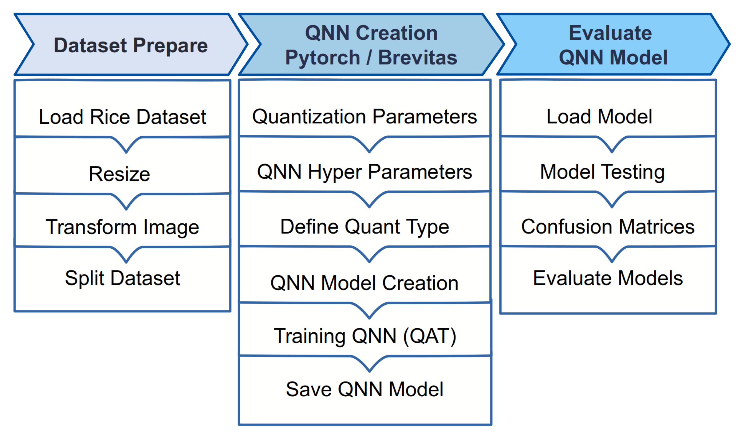
22] on MLP and Lenet-5 models. Each network quantizes the image input to 8 bits. In general, the complete workflow for each QNN is demonstrated in
Figure 1. The whole process for building a QNN network model consists of three steps, as presented in the figure. The first step includes the preparation of the dataset used by resizing the dimensions of the images from 3 × 256 × 256 to 3 × 32 × 32 in RGB format. This is then followed by dividing the dataset for training and validation. In the second step, the QNN network is created by determining the required parameters, such as weights and activation. Then, the hyperparameters are defined to be used for the training of the QNN model. The final step includes the evaluation of the constructed QNN models. Later, the performance results prove the efficiency of the proposed models. Performance comparisons with well-known existing studies indicate the superiority of the proposed study in terms of resource consumption. To sum up, the main contributions of this paper can be summarized by following:
The primary contribution is to develop a solution for an efficient classification strategy for rice variety classification, taking advantage of Quantized Neural Network (QNN) models.
The main emphasis has been placed on the utilization of limited resources for edge devices in IoT applications to reduce the high level of the computational burden of DL models.
The proposed QNN networks with various quantization levels benefit from the Pytorch framework and Xilinx Brevitas library on MLP and Lenet-5 models.
The performance efficiency of the proposed idea has been extensively tested using a real-world dataset with five different varieties, in comparison to state-of-the-art approaches.
The forthcoming parts of the article are organized as follows. The second part describes the definition of the models, including the dataset, performance measurement metrics, and the proposed QNN networks. In third section of the article, the performance evaluations are presented with a deep analysis. We finally conclude the paper in the last part.
2. Definition of Models
2.1. Preparation of Dataset
In this study, a recent dataset comprising five rice varieties (Ipsala, Arborio, Basmati, Yasemin, and Karacadagas as depicted in
Figure 2) is selected due to its high number of sample images [
23]. The number of samples for each class is 15,000, with a pixel size of 256 × 256.
A preprocessing is applied to resize the images to 32 × 32 as the main emphasis of this study is placed on the implementation of QNN models using resource-constrained devices. A view of both original and resized images can be seen in
Figure 3.
The advantage of reducing the size of the images on the LENET-5-based CNN model is presented in
Table 1, which shows the memory allocation, the number of parameters, and the billion floating point operations (GFLOPs) per second. With this reduction, the proposed model is capable of performing approximately 110 times less than the number of floating-point operations. Memory usage is also decreased almost 460 times. The dataset is partitioned into 60,000 images for training, 5000 images for validation, and 10,000 images for testing.
2.2. Multi-Layer Perceptron (MLP) Model
Multi-layer Perceptron Network (MLP) is a simple neural network with multiple hidden layers of perceptrons among the input and output layers [
24]. A typical MLP network is composed of a minimum of three layers beginning with an input layer to forward the processed data by the hidden layers to the output layer. The classification task is finalized by the output layer. The number of hidden layers is an application-specific property acting as computational units in a feed-forward fashion. In this study, the MLP network contains a flattened layer to shape the incoming image matrix in linear form. After linearization step, the one-dimensional data are fed to the next two hidden layers with 128 and 64 neurons. It is then captured by a Softmax layer with 5 outputs as the number of rice varieties to calculate the probability of membership for each rice class. The whole MLP model described is shown in
Figure 4.
2.3. LeNet-5 Model
LeNet-5 is a pioneering CNN structure that has had a great impact on the evolution of Deep Learning. It has the fundamental cells of CNN with a multi-layer convolution and pooling. In total, LeNet-5 comprises 7 layers with the exception of the input layer allowing the parameters to be trained in each layer. The input in this model is a 32 × 32-pixel image. The rationale behind the popularity of LeNet-5 is its simplicity and easy architecture. This study utilizes the original LeNet-5 model proposed in [
25] as depicted in
Figure 5.
2.4. Quantized Neural Network (QNN) Model
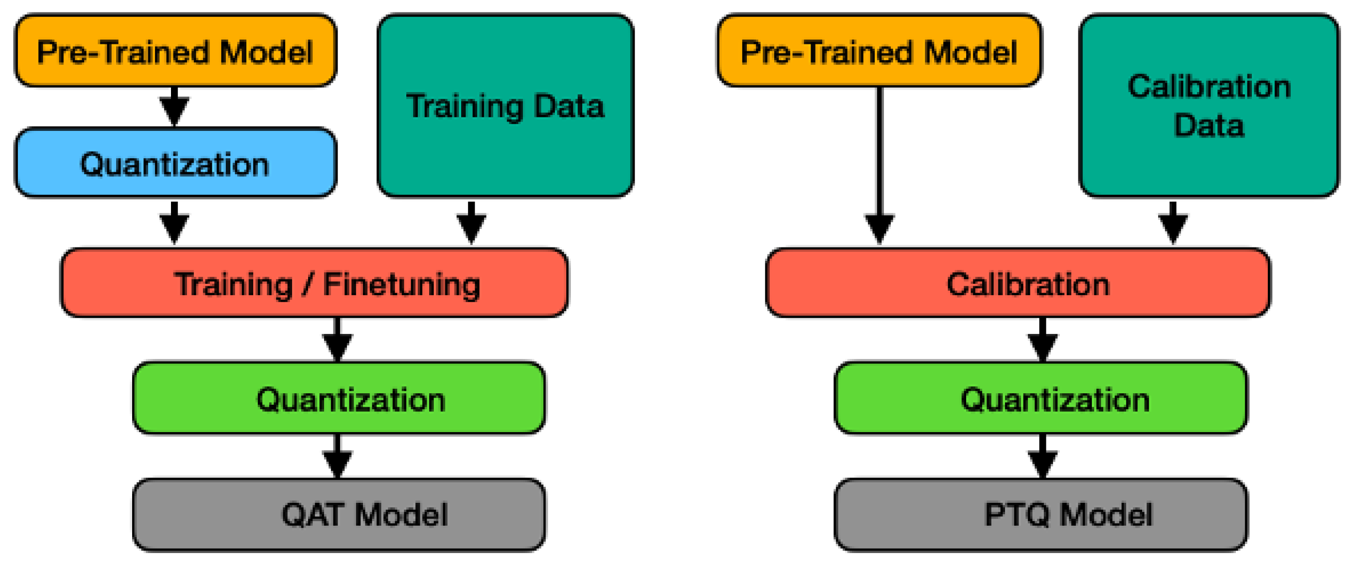
Quantization in DL models is defined as a process of reducing the memory requirement and computational burden by executing low-bit width values instead of floating-point values. To ensure a high-performance accuracy for applications run on-device, Quantization becomes a critical technique to supply a compact model leading to a reasonable size of neural network. Quantized Neural Network (QNN) is a special type of CNN without sacrificing performance. There are two types of quantization: Post-Training Quantization (PTQ) and Quantization-Aware-Training (QAT) [
26].
PTQ has a straightforward implementation process requiring no quantization in the training part benefitting from a pre-trained network. The parameters can be quantized based upon completion of the training of the floating-point network, subject to a quantization error on parameters. This may result in incorrect classification with increased quantization error. QAT is used to recover this error by computing the parameters during the training. As QAT performs the quantization process while training the model and calculating the parameters, one advantage of QAT is to raise the optimization to greater extents [
27]. The all steps of both quantization techniques are shown in
Figure 6.
CNN algorithms can include millions of floating-point parameters and billions of floating-point operations to recognize a single image [
28]. The winner of the ImageNet competition performed 244 MB of parameters and 1.4 GFLOPs in 2012 and 552 MB of parameters and 30.8 GFLOPs per image in 2014 [
29]. This requirement of high computing and memory capacities of deep neural networks hinders the utilization of these applications on mobile devices. To deal with this issue, quantization allows a model to consume less computing and memory resources while keeping its accuracy close to the original model [
30]. The quantization process is performed on the weight (W), input (I), bias (B), and output (O) data. The maximum value in the data to be quantized is calculated with the following equation.
N indicates the bit width to be quantized,
represents the maximum value to have occurred as a result of the quantization process. Here
is the value of the element with the highest absolute value according to the
i and
j indices of the matrix A to be quantized.
Then, a specific scale,
k, is defined by dividing
by
:
The quantization process is finalized, taking the ratio between
A and
k.
2.5. Quantization in Brevitas
Brevitas is a PyTorch library developed by Xilinx Research Lab for QAT-type quantification, introducing a quantized version of PyTorch layers. The layers in a neural network developed by PyTorch are replaced with Brevitas layers, resulting in the creation of the quantized model. Due to the interoperability of Brevitas with PyTorch layers, it makes the implementation of hybrid models feasible, thereby making the utilization of quantized and unquantized layers together. Consequently, this library quantizes the relevant parts of the layers with the parameters (W, I, B, O) aforementioned above. The frequently-used quantization techniques in Brevitas are:
INT: it returns the input tensor to the quantized integer at the specified bit width.
BINARY: it returns the input tensor quantized at (−1,1) values.
TERNARY: it returns the input tensor quantized at (−1,0,1).
Binary quantization represents the FP32 type in the W, I, B, O parameters as a 1-bit number. For example, after a bit quantization, the value of 0.127478 becomes 1, while the value of −0.05439 is quantized to −1. In the other quantization levels, the parameter value is converted to the closest number that can be represented by a selected number. The 4-bit quantization operation is shown on the matrix A given below as a numerical example.
It can be seen that after the quantization of the input matrix, its largest value is 8, and the smallest value is −7. These values are a range of signed numbers that can be written with a data width of 4 bits. In our study, quantization levels are used in WxAx format. Here, W represents the weight, A indicates the activation process, and x represents the bit width at which the quantization process will be performed.
This study implements BINARY for the W1A1 model and INT for the rest of the models. The networks developed for the MLP and Lenet-5 models are trained with quantized values at the W1A1, W2A2, W3A3, and W8A8 quantization levels. The complete process of building the MLP model is provided in Algorithm 1.
| Algorithm 1 MLP Quantize model generator algorithm |
- 1:
- 2:
- 3:
- 4:
- 5:
- 6:
- 7:
Require: Brevitas Modules (QuantIdentity,QuantLinear,Dropout,BatchNorm1D,TensorNorm) - 8:
procedureMLP - 9:
append QuantIdentity(I) to Model - 10:
append DropOut to Model - 11:
for outputFeatures do - 12:
append QuantLinear(W) to Model - 13:
append BatchNorm1D to Model - 14:
append QuantIdentity(A) to Model - 15:
append DropOut to Model - 16:
end for - 17:
append QuantLinear(W) to Model - 18:
append TensorNorm to Model - 19:
- 20:
for Model from MLP do - 21:
- 22:
end for - 23:
end procedure
|
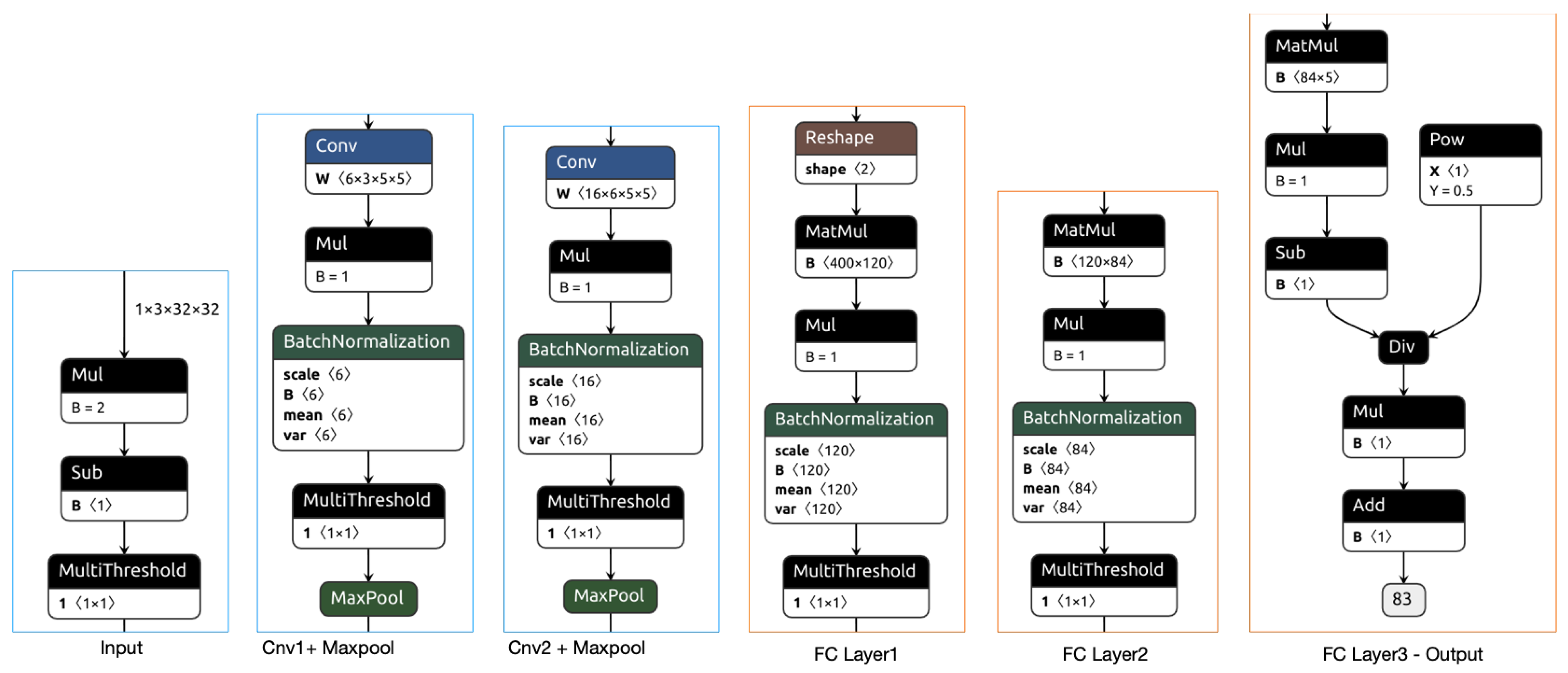
The trained QNN networks are converted to ONNX (Open Neural Network Exchange) format using the BrevitasToONNX module. The complete flowchart of the MLP model in ONNX format can be seen in
Figure 7.
In this figure, X represents the quantized input file of the output layer, which then takes Y as a power. In the input section, image data in the range of 0–255 is initially normalized to the range of −127–127. Then, the second normalization is performed on the normalized data to the range of (−1,1) with FP32 bit data type. In the second step, the linearized input matrix is multiplied by the weights on the 128-layer MLP block. It is then followed by multiple thresholding components and matrix transposing operations. After completing the same operations in the 64-layer MLP block, the classification scores are generated for the five rice grades.
The model created with the Brevitas library on the Lenet-5 model is seen in
Figure 8 after the ONNX transformation. In the introductory part of the Lenet-5-based QNN model, the image data are normalized in the range of (−1,1) in the FP32 bit data type. In the second and third transaction blocks, the QuntConv2d convolution layer, transpose operation, multi-threshold, and QuantMaxpool2d pooling operations are performed with the quantized data. At the entrance of the fourth block, the 2D matrix is flattened into 1D. After this stage, the operations made as in the quantified MLP model are performed. The pseudo-code of the entire Lenet-5 model is presented in Algorithm 2.
| Algorithm 2 LENET-5 quantize model generator algorithm |
- 1:
- 2:
- 3:
- 4:
- 5:
- 6:
- 7:
- 8:
Require: Brevitas Modules (QuantConv2d,MaxPool2D,QuantIdentity, - 9:
QuantLinear,BatchNorm2D,BatchNorm1D,TensorNorm) - 10:
procedureLenet - 11:
append QuantIdentity(I) to Model - 12:
for ConvFeatures do - 13:
append QuantConv2d(W) to Model - 14:
append BatchNorm2D to Model - 15:
append QuantIdentity(A) to Model - 16:
append MaxPool2D to Model - 17:
end for - 18:
for FcFeatures do - 19:
append QuantLinear(W) to Model - 20:
append BatchNorm1D to Model - 21:
append QuantIdentity(A) to Model - 22:
end for - 23:
append QuantLinear(W) to Model - 24:
append TensorNorm to Model - 25:
- 26:
for Model from Lenet do - 27:
- 28:
end for - 29:
end procedure
|
2.6. Performance Criterions
In the developed models of this study, the weight and activation parameters conduct the classification task at four different quantification levels. One of the most significant tools used in evaluating the performance of a model in AI-Based classification applications is the confusion matrix [
31]. It paves a way to explore the relationships between the performance and test outputs better. The knowledge regarding the accurate and inaccurate classification for both positive and negative samples can be obtained by the confusion matrix as presented in
Table 2 for a two-class confusion matrix.
Due to the five classes of rice in the dataset, the classification task of this study for each model includes a five-class confusion matrix. The terms of the confusion matrix are shown in
Table 3. The performances of the two models at all quantization levels are analyzed using the metrics of accuracy (ACC), precision (Pre), recall (Rec), F1-Score (F1S), operations per second, and memory usage. The metrics for each class in the multi-class confusion matrix can be calculated using the equations given below.
Accuracy denotes the success level of the classification. Precision stores the number of positive predictions, and Recall holds the number of positive samples to be identified. By combining precision and recall metrics, F1-Score is defined as the predictive ability through detailing a class-wise performance manner instead of accuracy that relies on the entire performance. The calculations of the values of TP, FP, TN, FN, and the criteria are shown by Algorithm 3.
| Algorithm 3 Multiclass Confusion Matrix Evaluate Algorithm |
- 1:
- 2:
- 3:
- 4:
for do - 5:
for do - 6:
if i is Not equal j then - 7:
- 8:
- 9:
end if - 10:
end for - 11:
- 12:
- 13:
- 14:
- 15:
- 16:
- 17:
end for - 18:
|
3. Experimental Results
This section presents the outputs of the classification process carried out by MLP ve Lenet-5 models. The dataset included as input in QNN models covers 75,000 rice images, and the size of each image is resized from 256 × 256 to 32 × 32. The names of the five rice varieties are Ipsala, Arborio, Basmati, Yasemin, and Karacadag, acting as classification outputs. The hardware specifications, software platforms, and hyperparameters are summarized in
Table 4 running on Google Colab.
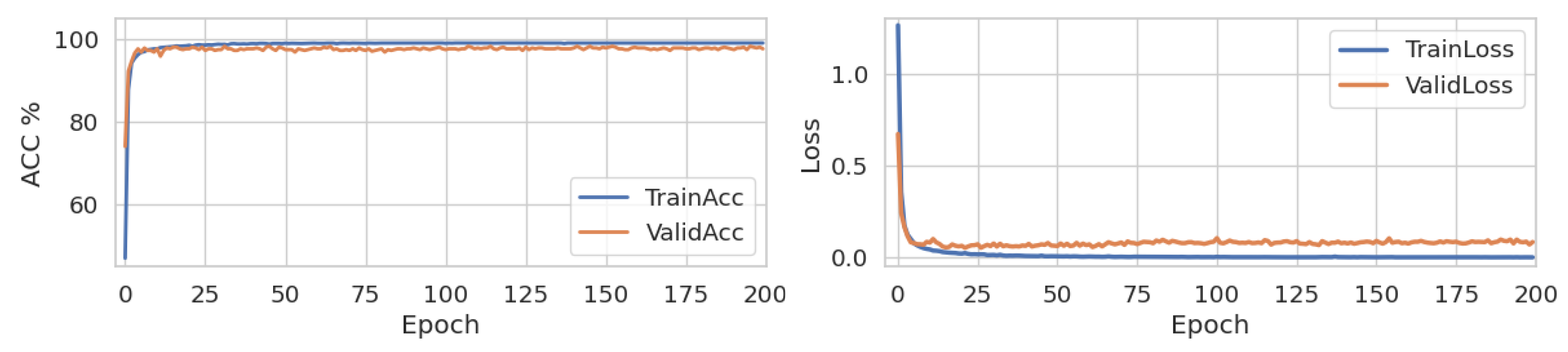
The first experiment presents the performance accuracy of the Lenet-5 model with no quantization. The models created with the dimension of 32 × 32 images on the Pytorch framework are trained for 200 epochs. In the model constructed by the MLP, the classification accuracy was obtained as 96.45%. The classification success of the model created by Lenet-5 reached 99.99% in the Lenet-5 model, as demonstrated in
Figure 9.
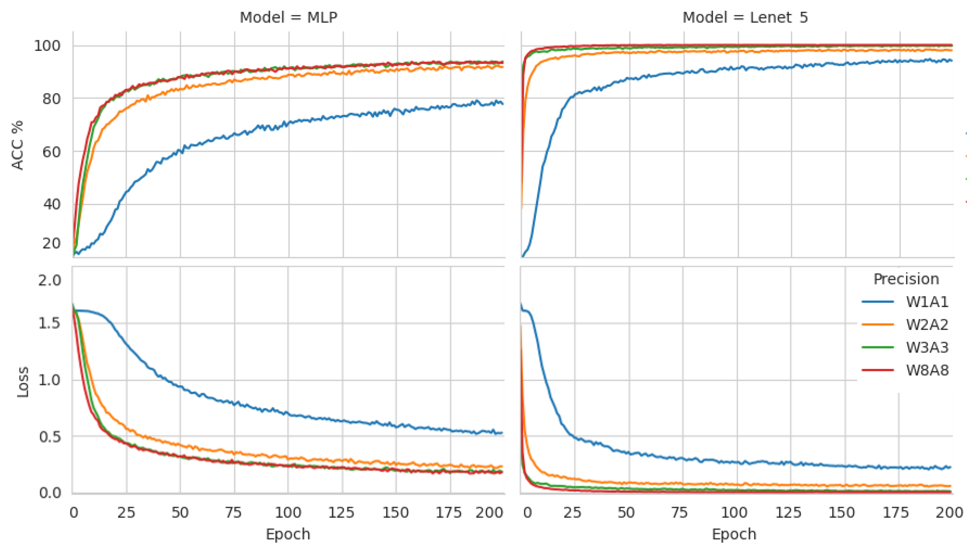
The next figure indicates the records of accuracy and loss values during the training phase for the two models at four quantization levels. These outputs are shown in
Figure 10 with a duration of 200 epochs. It is worth noting that all models in Lenet-5, with the exception of the 1-bit quantization model (W1A1), achieve a classification accuracy of nearly 98% for 50 epochs. The reason behind taking longer training time at a 1-bit quantization level is because of the low weight and activation sensitivity level in the backpropagation algorithm. We, therefore, set the training epoch duration as 200 for all models, in accordance with the duration at which the W1A1 model reached maximum learning. This permits us to visualize the results of all models on the same figure.
In total, 8 neural networks were trained according to the model and quantification levels with 60,000 training images and 5000 validation images in the dataset, and these network models were recorded with their weights. These eight network models were tested with 10,000 test images specifically dedicated to only the training phase. To compare the quantized neural networks with 32-bit floating point MLP and Lenet-5 networks, the same dataset was applied to test the performance. As a result of the test phase, the value of ACC, the amount of memory used, the weight and activation parameters of the model, and the number of billion transactions per second (GOPs) are presented in
Table 5. In this table, the first row of the models indexed by the FP32 term represents the models with no quantization. It is clearly seen that the accuracy of both models without quantization offers the best performance but at the expense of a very high memory usage property.
MLP-based models, as an overall trend, consume approximately seven times higher memory usage when compared with Lenet-5 models that achieve better accuracy. On the other hand, MLP-based quantized models attain 0.8 GOPs per second to quantize an image, while Lenet-5-based QNN models use 1.3 GOPs. QNN-W1A1 consumes only 7 KB of memory with a performance accuracy of 94.40%. However, MLP-FP32 achieves a similar performance accuracy using 1.6 MB memory which is almost 228 times larger than Lenet-5-W1A1. This particular result proves the superior practicality of the proposed model on resource-constrained edge devices. In addition, since the proposed model is suitable for data flow, it can reach very high speeds on parallel processing platforms such as FPGA. In this study, the highest efficiency in terms of memory consumption and accuracy was obtained in the Lenet-5-W3A3 network, with a memory consumption of 23 KB and an accuracy of 99.87%.
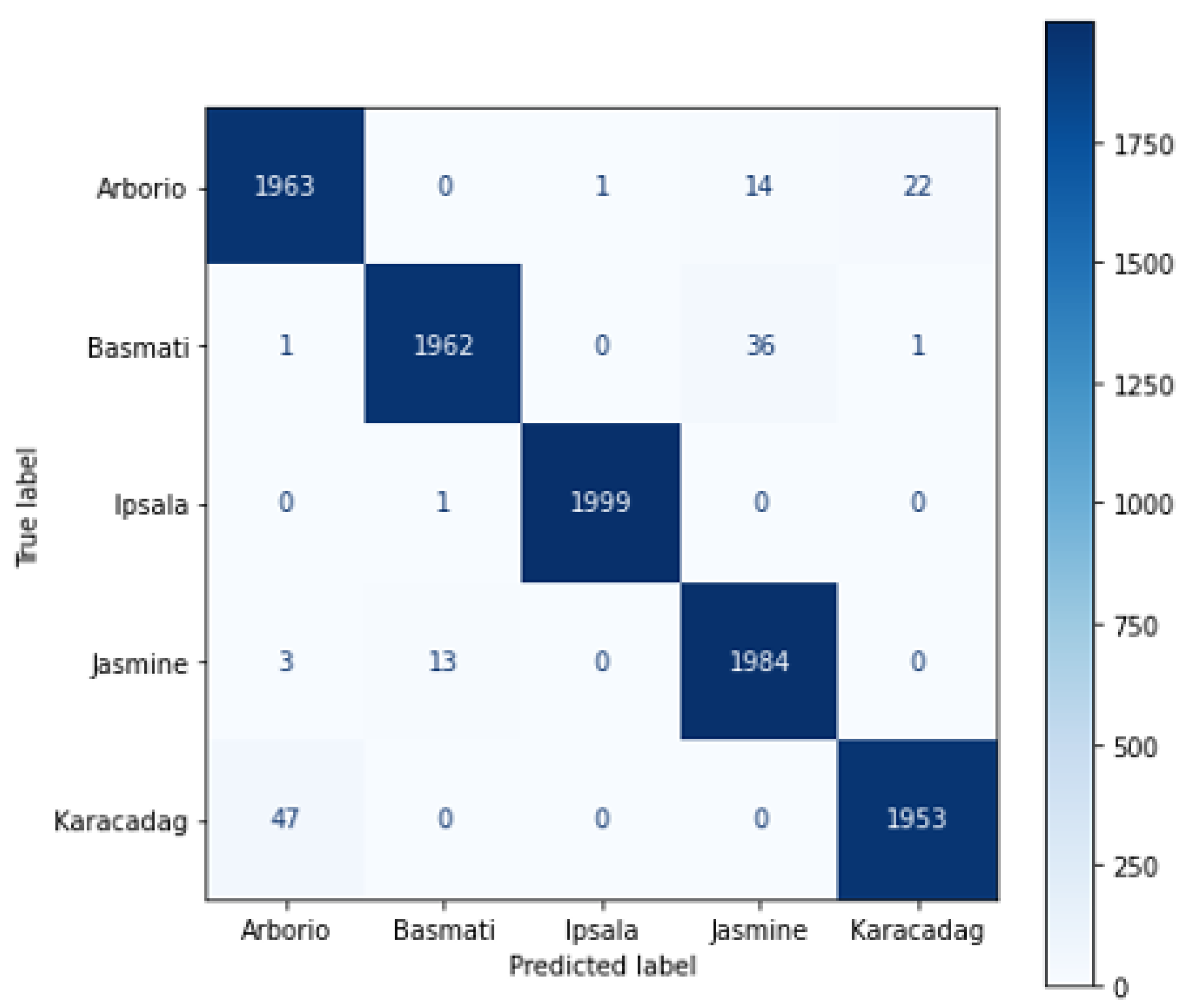
High accuracy when evaluating an AI model would partly indicate a proper success level of the network. For a full assessment of the network performance, the scores of Pre, Rec, and F1S are some examples of metrics to assess the reliability of the model. It can be inferred from these metrics that an inference regarding the performance accomplishment of the model is acquired. To extract these metrics, the confusion matrices for the eight QNN models are constructed from the statistical evaluation of the dataset. We chose to show the confusion matrices of the best and worst networks instead of presenting eight confusion matrices. The confusion matrix of the best network in terms of success/resource utilization ratio, Lenet-5-W3A3, is shown in
Figure 11. The accuracy for all rice types is similarly high, corresponding to a minor level of interference. In particular, for the Ipsala type, one sample is only classified wrongly.
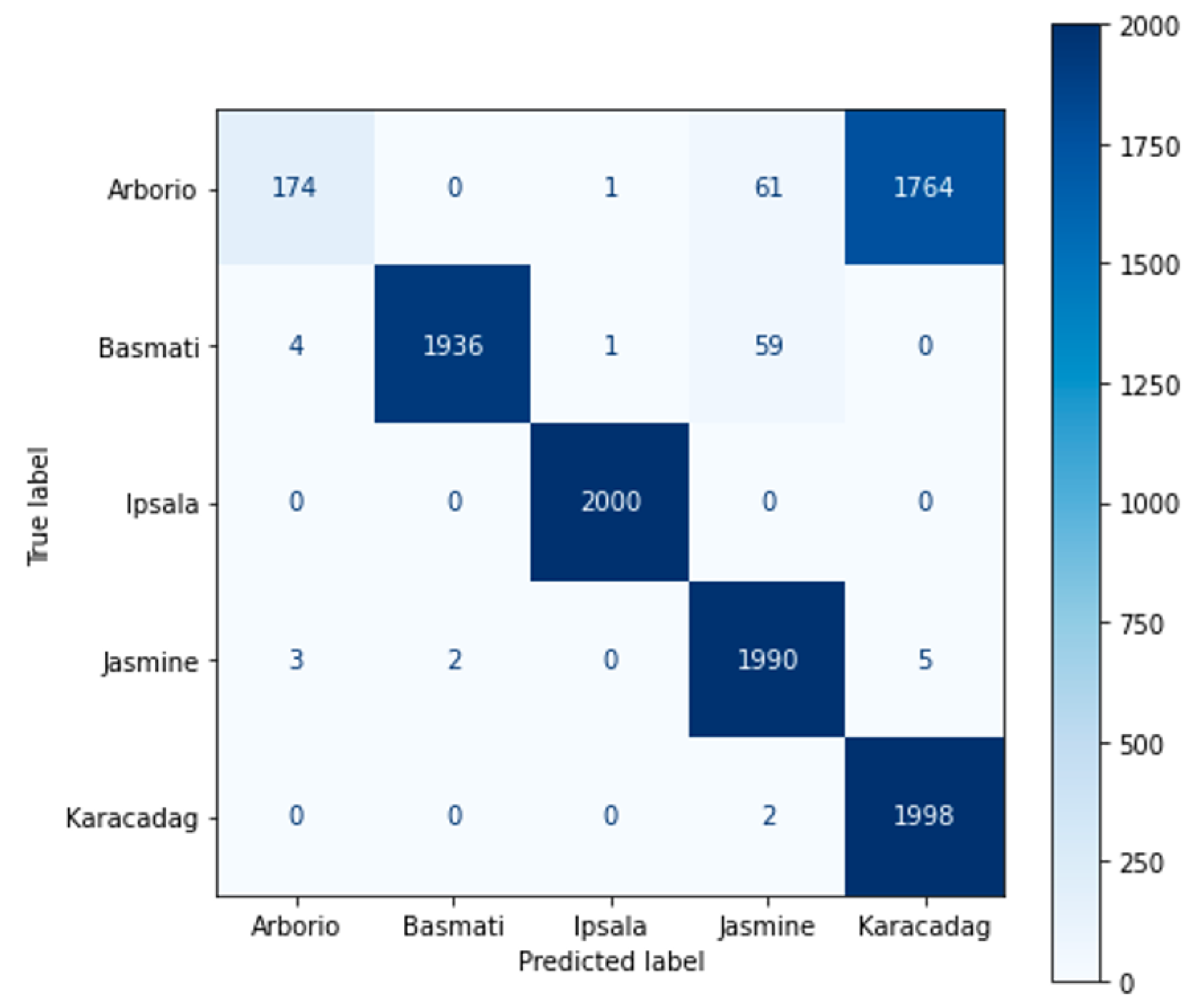
The confusion matrix of MLP-W1A1 exhibits the worst performance, as presented in
Figure 12. It is important mentioning that MLP-W1A1 actually overcomes the classification of four types with success. However, it has a terrifying classification accuracy for the Arborio type because an incorrect classification for 1764 Arborio samples was observed. Nevertheless, the total accuracy drops partly even though mislabeling of the majority of Arborio samples among 10,000 samples. To further analyze this error, the values of F1 for all classes are calculated using Algorithm-1, which is presented in
Table 6. The F1 scores confirm the suitability of the seven networks to be applied. On the one hand, although the MLP-W1A1 network approaches a performance accuracy close to 0.8, the network faces a very low F1 score of 0.16 caused by improper prediction of Arborio type, as outlined above. Ipsala type experiences the best F1 score, with almost all scores being equal to 1.
4. Conclusions and Discussion
This study investigates the potential of a high-performance classification approach through quantized deep learning for different rice varieties. The proposed idea has the key benefit of providing efficient and intelligent utilization of capacity in terms of memory, power, and processing speed. The main theme of the present work is, therefore, to design models running on edge devices that require low resource utilization. The confusion matrices of the developed models were constructed in connection with class-based F1 scores and accuracy levels. Eight Quantized Neural Network (QNN) networks were created using the environments of multilayer perceptron (MLP) and LeNet-5 with respect to various quantization levels. The results verify a successful classification of the seven models, except the MLP model at 1 quantization precision. We compare the results of the proposed best model with different studies in the literature as presented in
Table 7.
It is observed that most studies in classifying rice were carried out by using the Convolutional Neural Network (CNN) models with the examples of VGG-16, ResNet-50, and LeNet-5. Looking at
Table 7, the best classification accuracy is obtained by [
14] on VGG-16 with a 100% accuracy level consuming 537 MB memory and 30.9 GFLOPs. In our model, the Lenet-5-W3A3 model achieved 99.87% accuracy with only 23.1 Kb of memory and 1.3 GOPs processing. This reveals that the proposed model performs the classification with 23 times less processing and much less memory usage without sacrificing too much accuracy. Another model proposed by [
32] with an accuracy level of 99.5% is built on VGG-16 with 23 times more resource consumption than our study. To sum up
Table 7, as an overall trend, all compared schemes exhibit a high accuracy level at an unacceptable amount of memory usage and GFLOPs transactions for resource-limited edge devices. As a result, instead of an input image of 3 × 256 × 256 dimensions, the input image of 3 × 32 × 32 dimensions was quite sufficient for rice classification with this dataset. In addition, it is observed that Lenet-5, which is a simpler model compared to models such as VGG-16 and Resnet-50, successfully classifies this dataset. QNN models can be used by choosing the quantization level according to the source size and preferred accuracy level in the edge devices.


 ,
, 


