
Customized 2D CNN Model for the Automatic Emotion Recognition Based on EEG Signals

Abstract
:1. Introduction
- Collecting a comprehensive database of emotion recognition using musical stimulation based on EEG signals.
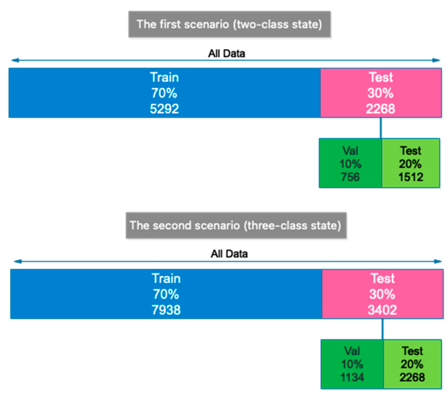
- Presenting an intelligent model based on deep learning in order to separate two and three basic emotional classes.
- Using end-to-end deep neural networks, which has led to the elimination of feature selection/extraction block diagram.
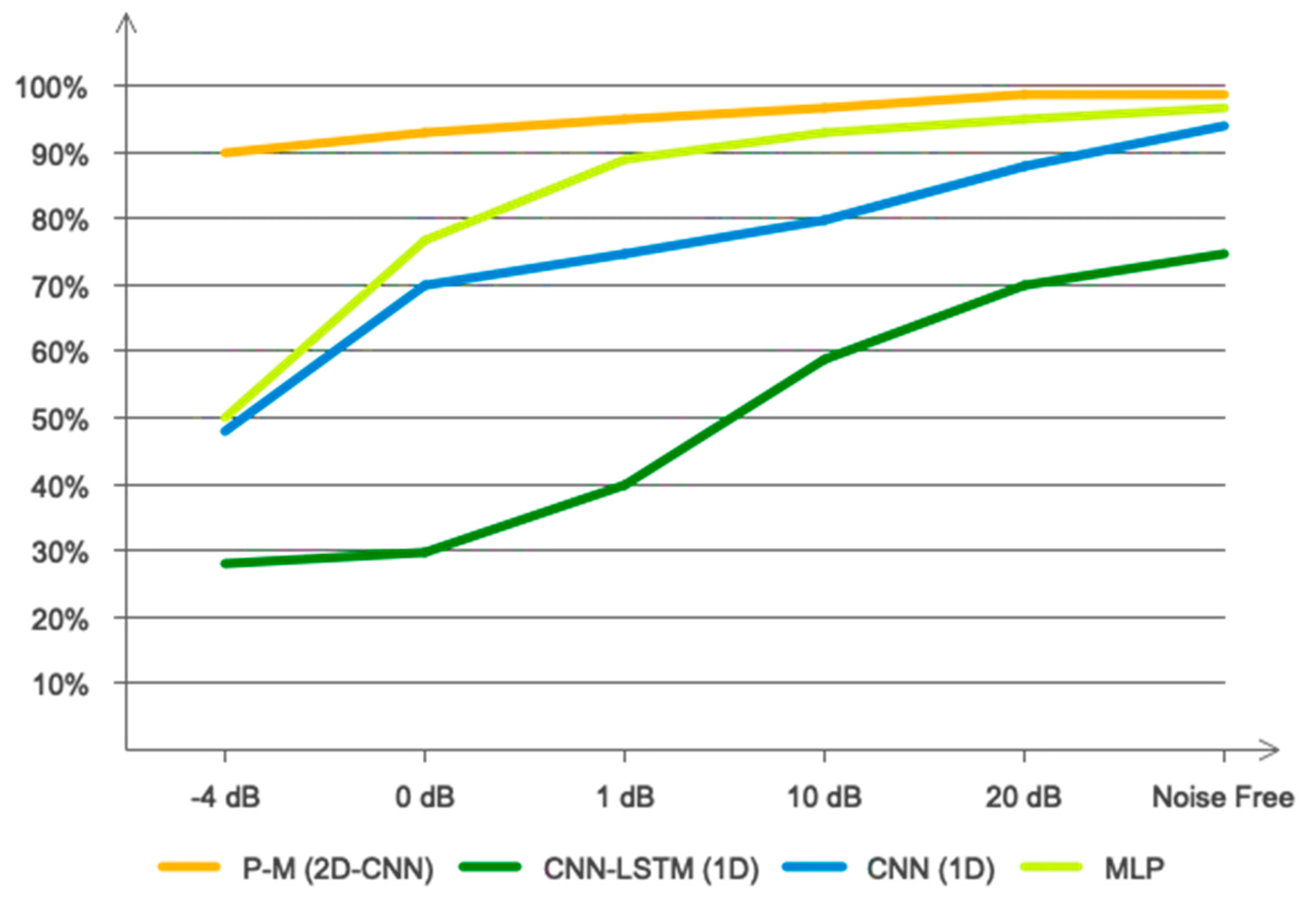
- Providing an algorithm based on deep convolutional networks that can be resistant to environmental noise to an acceptable extent.
- Presenting an automatic model that can classify two and three emotional classes with the highest accuracy and the least error compared with previous research.
2. Materials and Methods
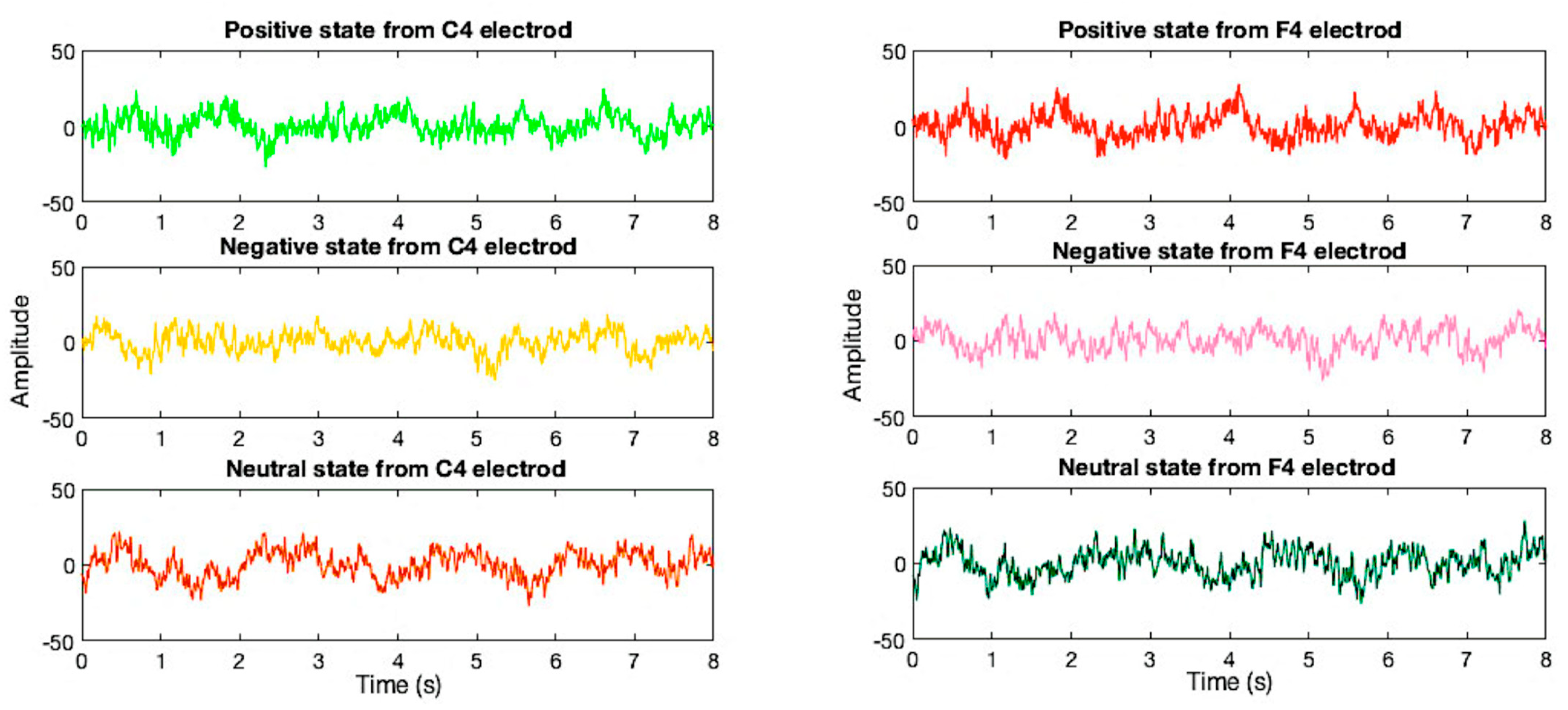
2.1. EEG Database Collection
2.2. Signal Processing Filters
2.2.1. Notch Filter
2.2.2. Butterworth Filter
2.3. Brief Description of Convolutional Neural Networks Model
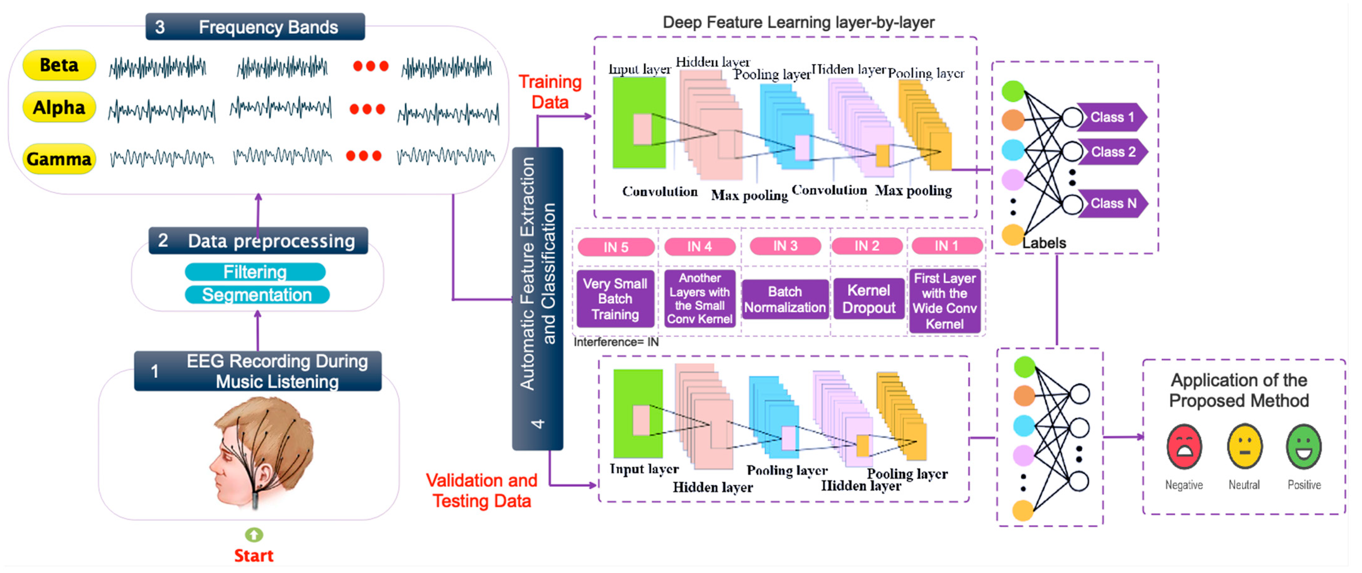
3. Proposed Deep Model
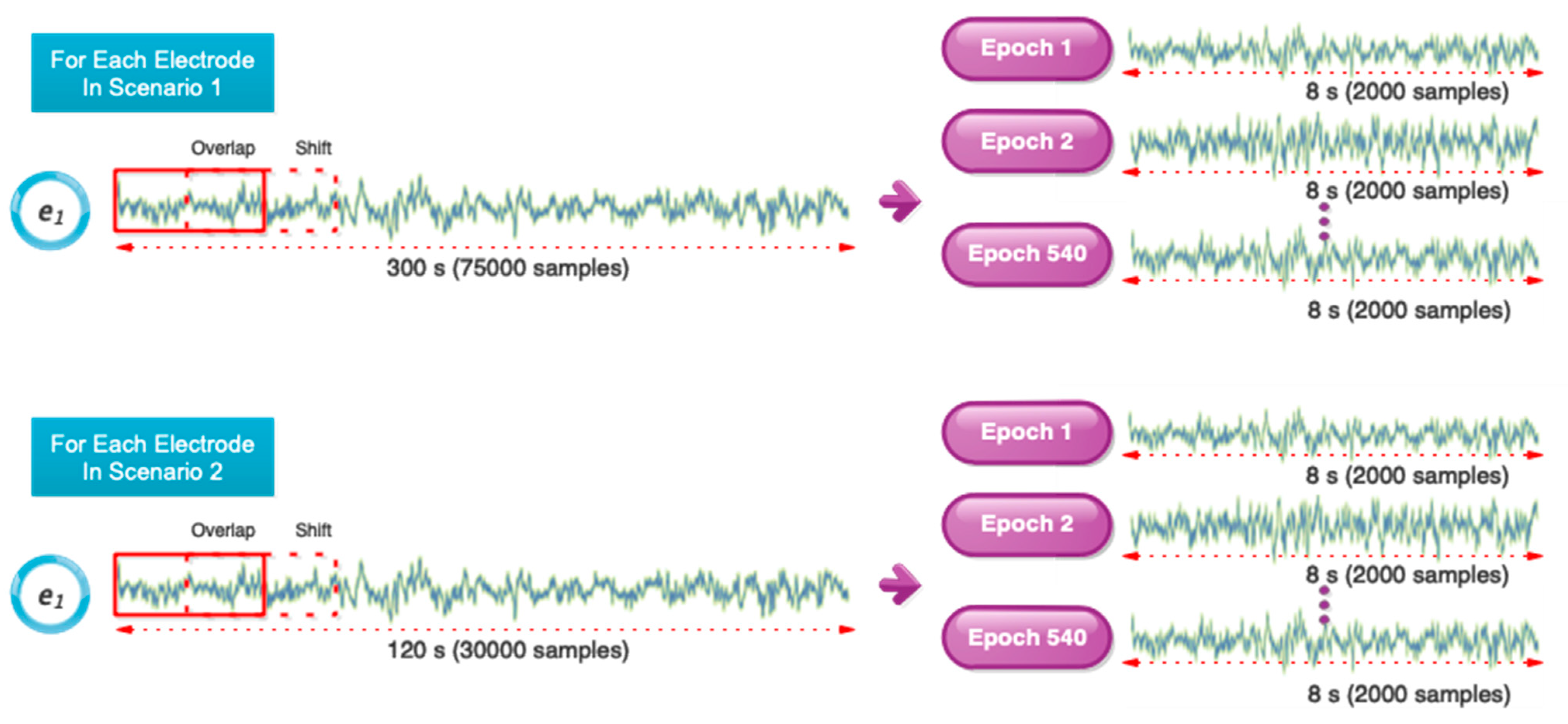
3.1. Data Pre-Processing
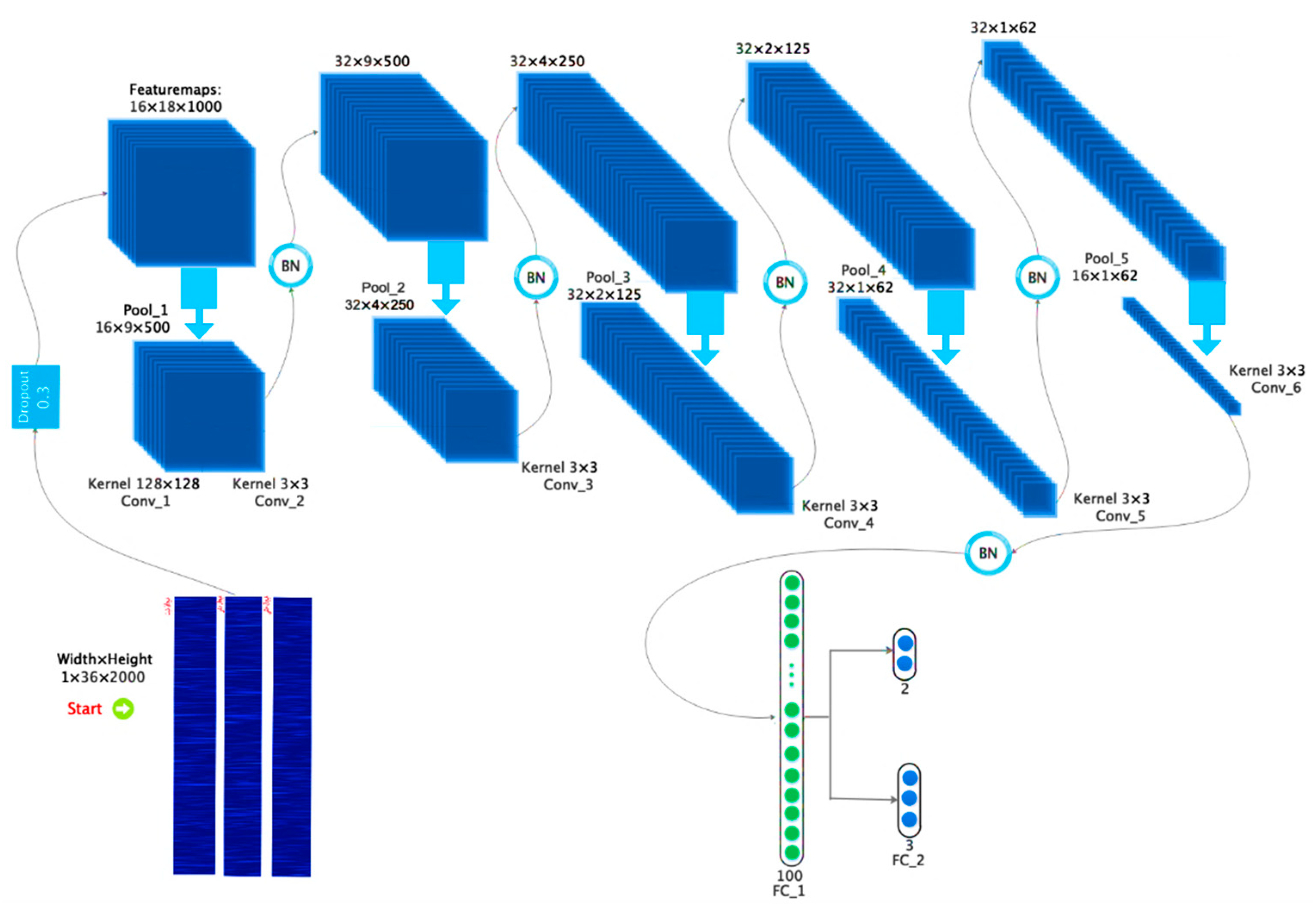
3.2. Deep Architectural Details
- I.
- One drop-out layer.
- II.
- A 2D Convolution layer with the Leaky-ReLu nonlinear function and a Max-Pooling layer with Batch Normalization are added.
- III.
- The architecture of the previous stage is repeated three more times.
- IV.
- A Convolution 2D layer is added with the Leaky-ReLu nonlinear function along with the Batch Normalization.
- V.
- The architecture of the previous stage is repeated one more time.
- VI.
- The output of the previous architecture is connected to the two Fully Connected layers, which are used in the last layer of the Softmax function to access the outputs and emotion recognition.
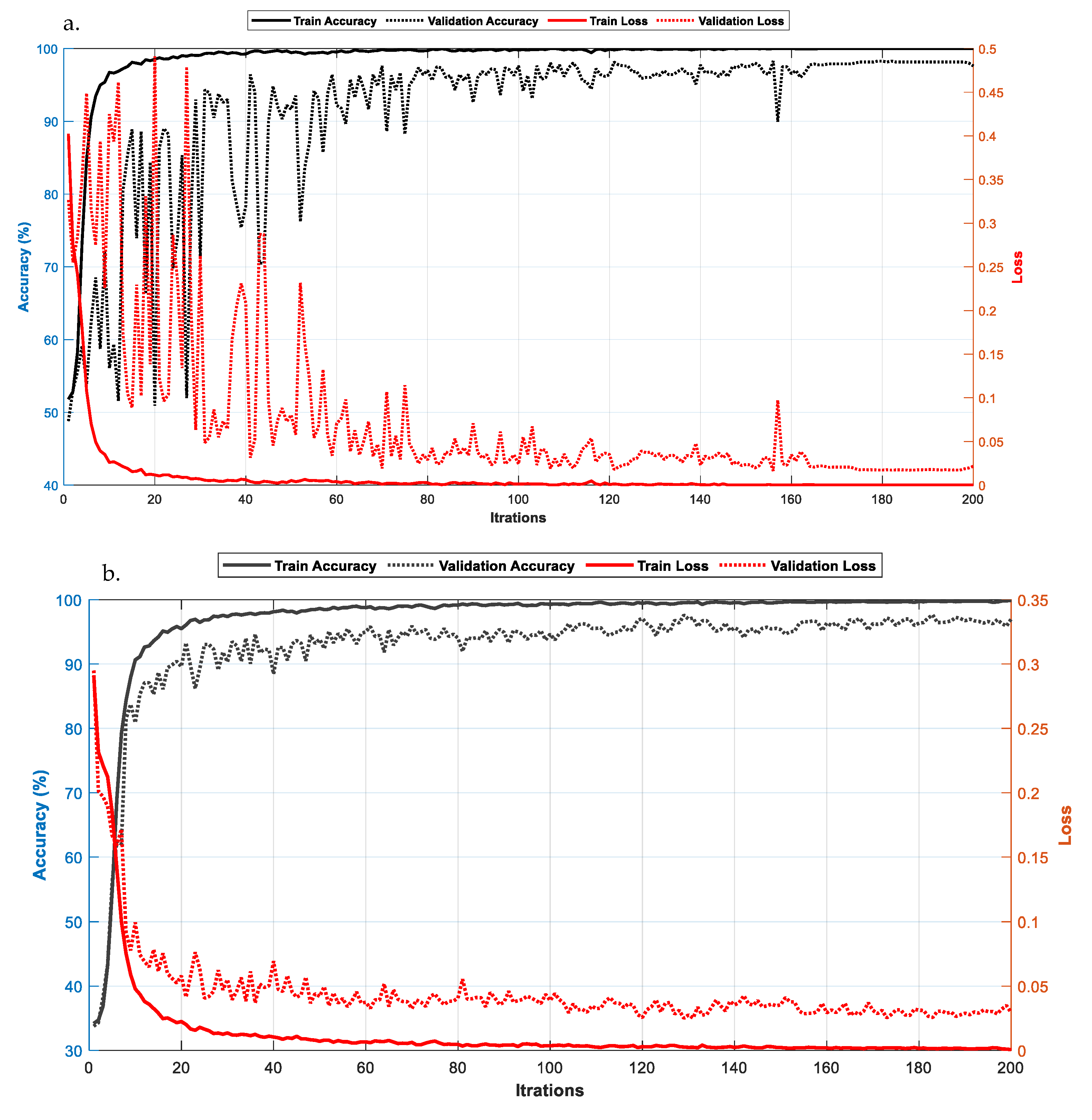
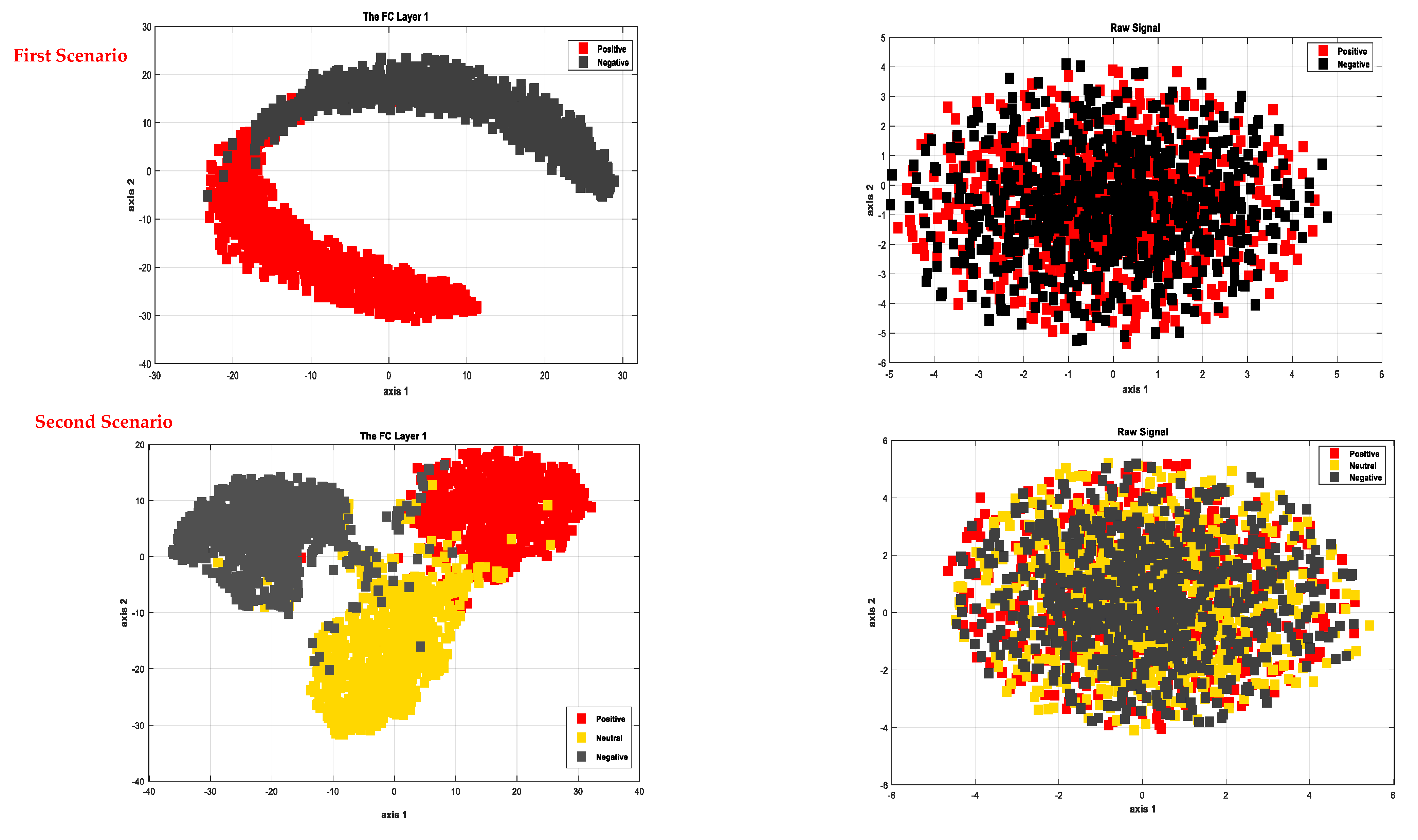
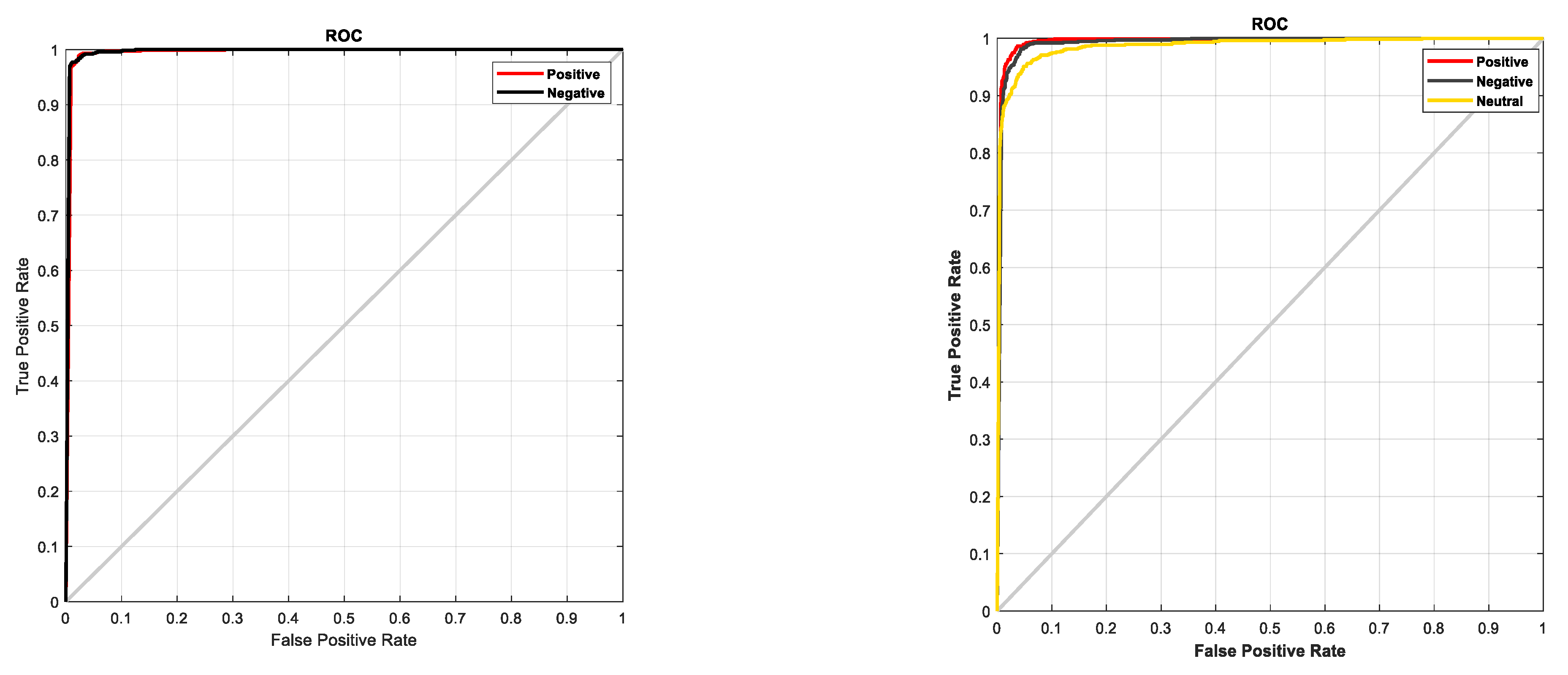
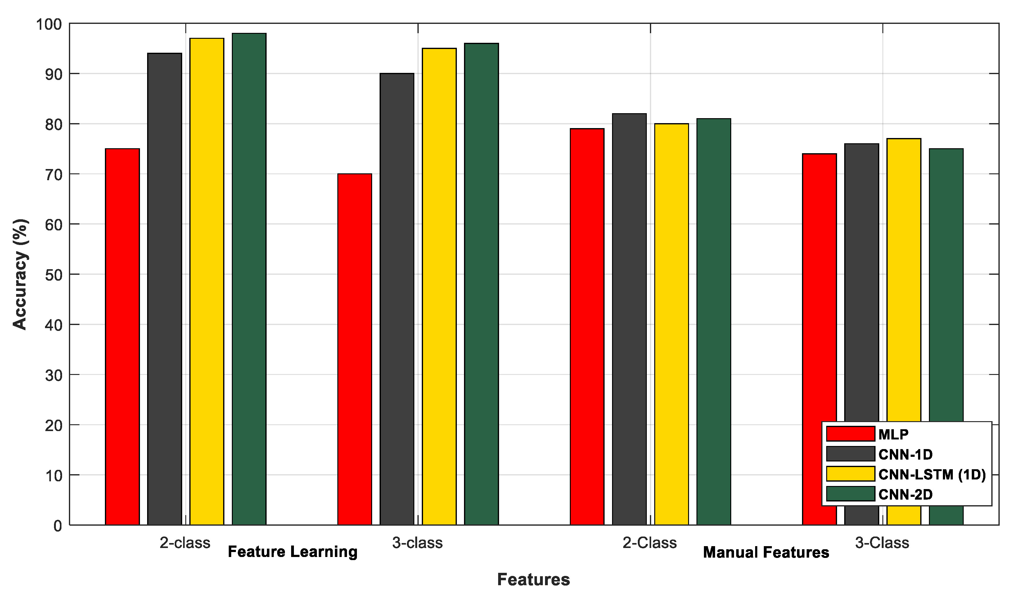
4. Experimental Results
5. Discussion
- Formalization of the robot’s internal emotional state: Adding emotional characteristics to agents and robots can increase their efficacy, adaptability, and plausibility. Determining neurocomputational models, formalizing them in already-existing cognitive architectures, modifying well-known cognitive models, or designing specialized emotional architectures has, thus, been the focus of robot design in recent years.
- Robotic emotional expression: In situations requiring complicated social interaction, such as assistive, educational, and social robotics, the capacity of robots to display recognisable emotional expressions has a significant influence on the social interaction that results.
- Robots’ capacity to discern human emotional state: Interacting with people would be improved if robots could discern and comprehend human emotions.
6. Conclusions
Author Contributions
Funding
Data Availability Statement
Conflicts of Interest
References
- Alswaidan, N.; Menai, M.E.B. A survey of state-of-the-art approaches for emotion recognition in text. Knowl. Inf. Syst. 2020, 62, 2937–2987. [Google Scholar] [CrossRef]
- Sheykhivand, S.; Rezaii, T.Y.; Meshgini, S.; Makoui, S.; Farzamnia, A. Developing a deep neural network for driver fatigue detection using EEG signals based on compressed sensing. Sustainability 2022, 14, 2941. [Google Scholar] [CrossRef]
- Sheykhivand, S.; Meshgini, S.; Mousavi, Z. Automatic detection of various epileptic seizures from EEG signal using deep learning networks. Comput. Intell. Electr. Eng. 2020, 11, 1–12. [Google Scholar]
- Dzedzickis, A.; Kaklauskas, A.; Bucinskas, V. Human emotion recognition: Review of sensors and methods. Sensors 2020, 20, 592. [Google Scholar] [CrossRef]
- Egger, M.; Ley, M.; Hanke, S. Emotion recognition from physiological signal analysis: A review. Electron. Notes Theor. Comput. Sci. 2019, 343, 35–55. [Google Scholar] [CrossRef]
- Jain, M.; Narayan, S.; Balaji, P.; Bhowmick, A.; Muthu, R.K. Speech emotion recognition using support vector machine. arXiv 2020, arXiv:2002.07590. [Google Scholar]
- Khalil, R.A.; Jones, E.; Babar, M.I.; Jan, T.; Zafar, M.H.; Alhussain, T. Speech emotion recognition using deep learning techniques: A review. IEEE Access 2019, 7, 117327–117345. [Google Scholar] [CrossRef]
- Ko, B.C. A brief review of facial emotion recognition based on visual information. Sensors 2018, 18, 401. [Google Scholar] [CrossRef]
- Lee, J.; Kim, S.; Kim, S.; Park, J.; Sohn, K. In Context-aware emotion recognition networks. In Proceedings of the IEEE/CVF International Conference on Computer Vision, Seoul, Republic of Korea, 27 October–2 November 2019; pp. 10143–10152. [Google Scholar]
- Li, X.; Song, D.; Zhang, P.; Zhang, Y.; Hou, Y.; Hu, B. Exploring EEG features in cross-subject emotion recognition. Front. Neurosci. 2018, 12, 162. [Google Scholar] [CrossRef]
- Liu, Z.-T.; Xie, Q.; Wu, M.; Cao, W.-H.; Mei, Y.; Mao, J.-W. Speech emotion recognition based on an improved brain emotion learning model. Neurocomputing 2018, 309, 145–156. [Google Scholar] [CrossRef]
- Poria, S.; Majumder, N.; Mihalcea, R.; Hovy, E. Emotion recognition in conversation: Research challenges, datasets, and recent advances. IEEE Access 2019, 7, 100943–100953. [Google Scholar] [CrossRef]
- Shu, L.; Xie, J.; Yang, M.; Li, Z.; Li, Z.; Liao, D.; Xu, X.; Yang, X. A review of emotion recognition using physiological signals. Sensors 2018, 18, 2074. [Google Scholar] [CrossRef] [PubMed]
- Swain, M.; Routray, A.; Kabisatpathy, P. Databases, features and classifiers for speech emotion recognition: A review. Int. J. Speech Technol. 2018, 21, 93–120. [Google Scholar] [CrossRef]
- Zhang, T.; Zheng, W.; Cui, Z.; Zong, Y.; Li, Y. Spatial–temporal recurrent neural network for emotion recognition. IEEE Trans. Cybern. 2018, 49, 839–847. [Google Scholar] [CrossRef] [PubMed]
- Li, X.; Hu, B.; Sun, S.; Cai, H. EEG-based mild depressive detection using feature selection methods and classifiers. Comput. Methods Programs Biomed. 2016, 136, 151–161. [Google Scholar] [CrossRef]
- Hou, Y.; Chen, S. Distinguishing different emotions evoked by music via electroencephalographic signals. Comput. Intell. Neurosci. 2019, 2019, 3191903. [Google Scholar] [CrossRef]
- Hasanzadeh, F.; Annabestani, M.; Moghimi, S. Continuous emotion recognition during music listening using EEG signals: A fuzzy parallel cascades model. Appl. Soft Comput. 2021, 101, 107028. [Google Scholar] [CrossRef]
- Keelawat, P.; Thammasan, N.; Numao, M.; Kijsirikul, B. Spatiotemporal emotion recognition using deep CNN based on EEG during music listening. arXiv 2019, arXiv:1910.09719. [Google Scholar]
- Chen, J.; Jiang, D.; Zhang, Y.; Zhang, P. Emotion recognition from spatiotemporal EEG representations with hybrid convolutional recurrent neural networks via wearable multi-channel headset. Comput. Commun. 2020, 154, 58–65. [Google Scholar] [CrossRef]
- Wei, C.; Chen, L.-L.; Song, Z.-Z.; Lou, X.-G.; Li, D.-D. EEG-based emotion recognition using simple recurrent units network and ensemble learning. Biomed. Signal Process. Control 2020, 58, 101756. [Google Scholar] [CrossRef]
- Sheykhivand, S.; Mousavi, Z.; Rezaii, T.Y.; Farzamnia, A. Recognizing emotions evoked by music using CNN-LSTM networks on EEG signals. IEEE Access 2020, 8, 139332–139345. [Google Scholar] [CrossRef]
- Er, M.B.; Çiğ, H.; Aydilek, İ.B. A new approach to recognition of human emotions using brain signals and music stimuli. Appl. Acoust. 2021, 175, 107840. [Google Scholar] [CrossRef]
- Gao, Q.; Yang, Y.; Kang, Q.; Tian, Z.; Song, Y. EEG-based emotion recognition with feature fusion networks. Int. J. Mach. Learn. Cybern. 2022, 13, 421–429. [Google Scholar] [CrossRef]
- Nandini, D.; Yadav, J.; Rani, A.; Singh, V. Design of subject independent 3D VAD emotion detection system using EEG signals and machine learning algorithms. Biomed. Signal Process. Control 2023, 85, 104894. [Google Scholar] [CrossRef]
- Niu, W.; Ma, C.; Sun, X.; Li, M.; Gao, Z. A Brain Network Analysis-Based Double Way Deep Neural Network for Emotion Recognition. IEEE Trans. Neural Syst. Rehabil. Eng. 2023, 31, 917–925. [Google Scholar] [CrossRef] [PubMed]
- Zali-Vargahan, B.; Charmin, A.; Kalbkhani, H.; Barghandan, S. Deep time-frequency features and semi-supervised dimension reduction for subject-independent emotion recognition from multi-channel EEG signals. Biomed. Signal Process. Control 2023, 85, 104806. [Google Scholar] [CrossRef]
- Hou, F.; Gao, Q.; Song, Y.; Wang, Z.; Bai, Z.; Yang, Y.; Tian, Z. Deep feature pyramid network for EEG emotion recognition. Measurement 2022, 201, 111724. [Google Scholar] [CrossRef]
- Smarr, K.L.; Keefer, A.L. Measures of depression and depressive symptoms: Beck depression Inventory-II (BDI-II), center for epidemiologic studies depression scale (CES-D), geriatric depression scale (GDS), hospital anxiety and depression scale (HADS), and patient health Questionnaire-9 (PHQ-9). Arthritis Care Res. 2011, 63, S454–S466. [Google Scholar]
- Mojiri, M.; Karimi-Ghartemani, M.; Bakhshai, A. Time-domain signal analysis using adaptive notch filter. IEEE Trans. Signal Process. 2006, 55, 85–93. [Google Scholar] [CrossRef]
- Robertson, D.G.E.; Dowling, J.J. Design and responses of Butterworth and critically damped digital filters. J. Electromyogr. Kinesiol. 2003, 13, 569–573. [Google Scholar] [CrossRef]
- Kattenborn, T.; Leitloff, J.; Schiefer, F.; Hinz, S. Review on Convolutional Neural Networks (CNN) in vegetation remote sensing. ISPRS J. Photogramm. Remote Sens. 2021, 173, 24–49. [Google Scholar] [CrossRef]
- Novakovsky, G.; Dexter, N.; Libbrecht, M.W.; Wasserman, W.W.; Mostafavi, S. Obtaining genetics insights from deep learning via explainable artificial intelligence. Nat. Rev. Genet. 2023, 24, 125–137. [Google Scholar] [CrossRef] [PubMed]
- Khaleghi, N.; Rezaii, T.Y.; Beheshti, S.; Meshgini, S.; Sheykhivand, S.; Danishvar, S. Visual Saliency and Image Reconstruction from EEG Signals via an Effective Geometric Deep Network-Based Generative Adversarial Network. Electronics 2022, 11, 3637. [Google Scholar] [CrossRef]
- Wang, J.; Wang, M. Review of the emotional feature extraction and classification using EEG signals. Cogn. Robot. 2021, 1, 29–40. [Google Scholar] [CrossRef]
- Mouley, J.; Sarkar, N.; De, S. Griffith crack analysis in nonlocal magneto-elastic strip using Daubechies wavelets. Waves Random Complex Media 2023, 1–19. [Google Scholar] [CrossRef]
- Zhao, H.; Ye, N.; Wang, R. Improved Cross-Corpus Speech Emotion Recognition Using Deep Local Domain Adaptation. Chin. J. Electron. 2023, 32, 1–7. [Google Scholar]
- Chanel, G.; Rebetez, C.; Bétrancourt, M.; Pun, T. Emotion assessment from physiological signals for adaptation of game difficulty. IEEE Trans. Syst. Man Cybern.-Part A Syst. Hum. 2011, 41, 1052–1063. [Google Scholar] [CrossRef]
- Sabahi, K.; Sheykhivand, S.; Mousavi, Z.; Rajabioun, M. Recognition COVID-19 cases using deep type-2 fuzzy neural networks based on chest X-ray image. Comput. Intell. Electr. Eng. 2023, 14, 75–92. [Google Scholar]
- Shahini, N.; Bahrami, Z.; Sheykhivand, S.; Marandi, S.; Danishvar, M.; Danishvar, S.; Roosta, Y. Automatically Identified EEG Signals of Movement Intention Based on CNN Network (End-To-End). Electronics 2022, 11, 3297. [Google Scholar] [CrossRef]


| Subject | 1 | 2 | 3 | 4 | 5 | 6 | 7 | 8 | 9 | 10 | 11 | 12 | 13 | 14 | 15 | 16 |
|---|---|---|---|---|---|---|---|---|---|---|---|---|---|---|---|---|
| Sex | M | M | F | M | M | M | M | M | M | F | F | F | F | M | F | M |
| Age | 25 | 24 | 27 | 24 | 32 | 18 | 25 | 29 | 30 | 19 | 18 | 20 | 22 | 24 | 23 | 28 |
| BDI | 16 | 22 | 19 | 4 | 0 | 11 | 13 | 19 | 20 | 14 | 22 | 12 | 0 | 12 | 1 | 9 |
| Valence for P emotion | 9 | 6.8 | 6.2 | 7.4 | 5.8 | 5.6 | 7.2 | 7.8 | 7.4 | 6.8 | 7.8 | 8.6 | 6 | 8 | - | 7.4 |
| Arousal for P emotion | 9 | 6.2 | 7.4 | 7.6 | 5 | 5.4 | 7.4 | 7.4 | 7 | 6.6 | 8 | 8.6 | 6 | 8 | - | 8 |
| Valence for N emotion | 2 | 3.6 | 4.2 | 2.4 | 4.4 | 2 | 3.8 | 2.8 | 3.4 | 3.8 | 4.5 | 2 | 2 | 1.8 | - | 1.8 |
| Arousal for N emotion | 1 | 2 | 4.6 | 2.6 | 5.6 | 1.6 | 3.8 | 3 | 5.4 | 3.2 | 3 | 1.2 | 1.2 | 1.6 | - | 2 |
| Result of Test | ACC | REJ | REJ | ACC | REJ | REJ | REJ | ACC | REJ | REJ | REJ | ACC | ACC | ACC | REJ | ACC |
| Reason for rejection | - | Depressed 21 < 22 | Failure in the SAM test | - | Failure in the SAM test | Failure in the P emotion | Failure in the N emotion | - | Failure in the N emotion | Failure in the N emotion | Depressed 21 < 22 | - | - | - | Motion noise | - |
| Emotion Sign and Music Number | The Type of Emotion Created in the Subject | The Name of the Music |
|---|---|---|
| N1 | Negative | Advance Income of Isfahan |
| P1 | Positive | Azari 6/8 |
| N2 | Negative | Advance Income of Homayoun |
| P2 | Positive | Azari 6/8 |
| P3 | Positive | Bandari 6/8 |
| N3 | Negative | Afshari piece |
| N4 | Negative | Advance Income of Isfahan |
| P4 | Positive | Persian 6/8 |
| N5 | Negative | Advance Income of Dashti |
| P5 | Positive | Bandari 6/8 |
| Padding | Number of Filters | Strides | Size of Kernel and Pooling | Output Shape | Activation Function | Layer Type | L |
|---|---|---|---|---|---|---|---|
| Yes | 16 | 2 | 128 × 128 | (None, 18, 1000, 16) | Leaky ReLU | Convolution 2-D | 0–1 |
| No | - | 2 | 2 × 2 | (None, 9, 500, 16) | - | Max-Pooling 2-D | 1–2 |
| Yes | 32 | 1 | 3 × 3 | (None, 9, 500, 32) | Leaky ReLU | Convolution 2-D | 2–3 |
| No | - | 2 | 2 × 2 | (None, 4, 250, 32) | - | Max-Pooling 2-D | 3–4 |
| Yes | 32 | 1 | 3 × 3 | (None, 4, 250, 32) | Leaky ReLU | Convolution 2-D | 4–5 |
| No | - | 2 | 2 × 2 | (None, 2, 125, 32) | - | Max-Pooling 2-D | 5–6 |
| Yes | 32 | 1 | 3 × 3 | (None, 2, 125, 32) | Leaky ReLU | Convolution 2-D | 6–7 |
| No | - | 2 | 2 × 2 | (None, 1, 62, 32) | - | Max-Pooling 2-D | 7–8 |
| Yes | 32 | 1 | 3 × 3 | (None, 1, 62, 32) | Leaky ReLU | Convolution 2-D | 8–9 |
| Yes | 16 | 1 | 3 × 3 | (None, 1, 62, 16) | Leaky ReLU | Convolution 2-D | 10–11 |
| - | - | - | - | (None, 100) | Leaky ReLU | FC | 11–12 |
| - | - | - | - | (None, 2–3) | Softmax | FC | 12–13 |
| Parameters | Search Space | Optimal Value | |
| Optimizer | RMSProp, Adam, Sgd, Adamax, and Adadelta | RMSProp | |
| Cost function | MSE, Cross-entropy | Cross-Entropy | |
| Number of | Convolution layers | 3, 5, 6, 11, 15 | 6 |
| Filters in the first convolution layer | 16, 32, 64, 128 | 16 | |
| Filters in the second convolution layer | 16, 32, 64, 128 | 32 | |
| Filters in other convolution layers | 16, 32, 64, 128 | 32 | |
| Size of filter in the | First convolution layer | 3, 16, 32, 64, 128 | 128 |
| Other convolution layers | 3, 16, 32, 64, 128 | 3 | |
| Dropout rate | Before the first convolution layer | 0, 0.2, 0.3, 0.4, 0.5 | 0.3 |
| After the first convolution layer | 0, 0.2, 0.3, 0.4, 0.5 | 0.3 | |
| Batch size | 4, 8, 10, 16, 32, 64 | 10 | |
| Learning rate | 0.01, 0.001, 0.0001 | 0. 001 |
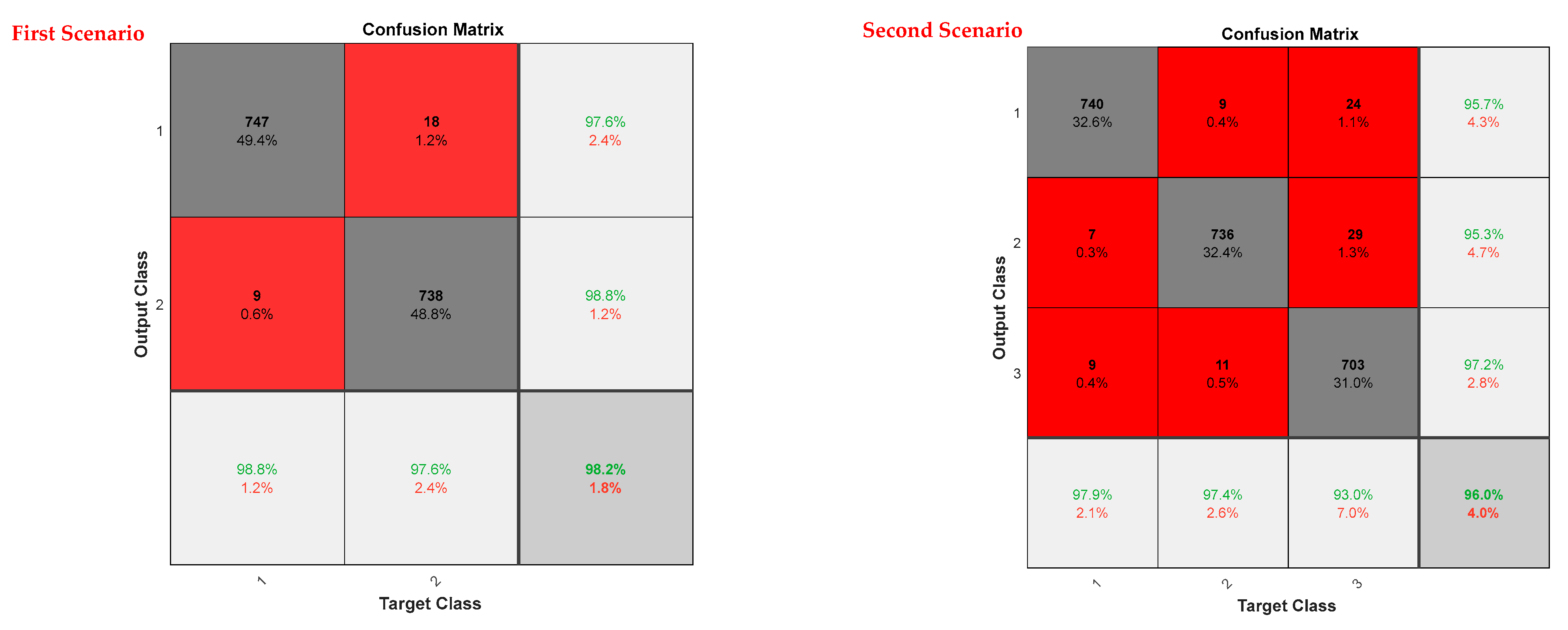
| First Scenario (P and N) | Positive | Negative | |
|---|---|---|---|
| Sensitivity | 98.2 | 98.2 | |
| Accuracy | 98.8 | 97.6 | |
| Specificity | 97.6 | 98.8 | |
| Precision | 97.6 | 98.8 | |
| Second Scenario | Positive | Negative | Neutral |
| Sensitivity | 97.8 | 97.5 | 96.7 |
| Accuracy | 95.7 | 95.3 | 97.2 |
| Specificity | 98.9 | 98.6 | 96.5 |
| Precision | 97.9 | 97.4 | 93 |
| Study | Stimulus | Methods | Number of Emotions Considered | ACC% |
|---|---|---|---|---|
| Zhao et al. [37] | Music | Deep local domain | 4 | 89 |
| Chanel et al. [38] | Video Games | Frequency bands extraction | 3 | 63 |
| Jirayucharoensak et al. [39] | Video Clip | Principal component analysis | 3 | 49.52 |
| Er et al. [23] | Music | VGG16 | 4 | 74 |
| Sheykhivand et al. [22] | Music | CNN-LSTM | 3 | 96 |
| Hou et al. [28] | Video Clip | FPN+SVM | 4 | 95.50 |
| Proposed model | Music | Customized CNN | 3 | 98 |
| Model | Feature Learning | Eng. Features | ||
|---|---|---|---|---|
| First Scenario | Second Scenario | First Scenario | Second Scenario | |
| MLP | 75% | 70% | 79% | 74% |
| 1D-CNN | 94% | 90% | 82% | 76% |
| CNN-LSTM | 97% | 95% | 80% | 77% |
| 2D-CNN | 98% | 96% | 81% | 75% |
Disclaimer/Publisher’s Note: The statements, opinions and data contained in all publications are solely those of the individual author(s) and contributor(s) and not of MDPI and/or the editor(s). MDPI and/or the editor(s) disclaim responsibility for any injury to people or property resulting from any ideas, methods, instructions or products referred to in the content. |
© 2023 by the authors. Licensee MDPI, Basel, Switzerland. This article is an open access article distributed under the terms and conditions of the Creative Commons Attribution (CC BY) license (https://creativecommons.org/licenses/by/4.0/).
Share and Cite
Baradaran, F.; Farzan, A.; Danishvar, S.; Sheykhivand, S. Customized 2D CNN Model for the Automatic Emotion Recognition Based on EEG Signals. Electronics 2023, 12, 2232. https://doi.org/10.3390/electronics12102232
Baradaran F, Farzan A, Danishvar S, Sheykhivand S. Customized 2D CNN Model for the Automatic Emotion Recognition Based on EEG Signals. Electronics. 2023; 12(10):2232. https://doi.org/10.3390/electronics12102232
Chicago/Turabian StyleBaradaran, Farzad, Ali Farzan, Sebelan Danishvar, and Sobhan Sheykhivand. 2023. "Customized 2D CNN Model for the Automatic Emotion Recognition Based on EEG Signals" Electronics 12, no. 10: 2232. https://doi.org/10.3390/electronics12102232