Article

Signature and Log-Signature for the Study of Empirical Distributions Generated with GANs

1
Centre for Intelligent Multidimensional Data Analysis, HK Science Park, Shatin, Hong Kong, China
2
Departamento de Informática de Sistemas y Computadores, Universitat Politècnica de València, 46022 València, Spain
3
Informatik und Mathematik, GOETHE—University Frankfurt am Main, 60323 Frankfurt am Main, Germany
4
Estudis d’Informàtica, Multimèdia i Telecomunicació, Universitat Oberta de Catalunya, 08018 Barcelona, Spain
5
HESSIAN Center for AI (hessian.AI), 64293 Darmstadt, Germany
*
Author to whom correspondence should be addressed.
Electronics 2023, 12(10), 2192; https://doi.org/10.3390/electronics12102192
Submission received: 19 April 2023 / Revised: 4 May 2023 / Accepted: 8 May 2023 / Published: 11 May 2023

Abstract

:
In this paper, we address the research gap in efficiently assessing Generative Adversarial Network (GAN) convergence and goodness of fit by introducing the application of the Signature Transform to measure similarity between image distributions. Specifically, we propose the novel use of Root Mean Square Error (RMSE) and Mean Absolute Error (MAE) Signature, along with Log-Signature, as alternatives to existing methods such as Fréchet Inception Distance (FID) and Multi-Scale Structural Similarity Index Measure (MS-SSIM). Our approach offers advantages in terms of efficiency and effectiveness, providing a comprehensive understanding and extensive evaluations of GAN convergence and goodness of fit. Furthermore, we present innovative analytical measures based on statistics by means of Kruskal–Wallis to evaluate the goodness of fit of GAN sample distributions. Unlike existing GAN measures, which are based on deep neural networks and require extensive GPU computations, our approach significantly reduces computation time and is performed on the CPU while maintaining the same level of accuracy. Our results demonstrate the effectiveness of the proposed method in capturing the intrinsic structure of the generated samples, providing meaningful insights into GAN performance. Lastly, we evaluate our approach qualitatively using Principal Component Analysis (PCA) and adaptive t-Distributed Stochastic Neighbor Embedding (t-SNE) for data visualization, illustrating the plausibility of our method.

1. Introduction

Generative Adversarial Networks (GANs) [1] have gained significant attention in recent years as a powerful tool for generating realistic synthetic images, with a wide range of applications in computer vision [2,3], graphics [4,5], and Machine Learning (ML) [6,7]. Despite their remarkable successes, assessing the quality of the generated samples and measuring the convergence of GANs remain challenging tasks. Existing metrics, such as Fréchet Inception Distance (FID) [8] and Multi-Scale Structural Similarity Index Measure (MS-SSIM) [9] have been widely used, but they suffer from certain limitations. These limitations include the requirement of substantial computational resources and time, dependence on specific Deep Learning (DL) architectures, and limited interpretability, which restrict their practical applicability and hinder further advancements in the field.
To address these challenges, there is a pressing need for a novel approach that can efficiently and effectively assess GAN-generated images while maintaining the same level of accuracy as existing metrics. Moreover, such an approach should provide a deeper understanding of the underlying distributions of the generated samples and be applicable across different GAN architectures and problem domains.
In this paper, we present a novel approach to study empirical distributions generated with GANs, leveraging the well-established Signature Transform and Log-Signature as powerful mathematical tools [10,11,12,13]. Our work is the first to introduce the use of Root Mean Square Error (RMSE) and Mean Absolute Error (MAE) Signature, along with Log-Signature, as alternatives for measuring GAN convergence. Furthermore, we propose the application of analytical measures based on statistics to study the goodness of fit of the GAN sample distribution, which are both efficient and effective. In contrast to existing GAN metrics that involve considerable GPU-based computation, our approach significantly reduces computation time and resources while maintaining the same level of accuracy.
We propose a two-fold approach. First, we introduce a score function based on the Signature Transform [14] to evaluate image quality in a novel manner, offering reliability, speed, and ease of computation for each epoch. Second, we employ statistical techniques to study the goodness of fit of the generated distribution, providing a standardized pipeline for interpreting the results of the converged sample distribution. A key contribution of this paper is the introduction of Kruskal–Wallis for GAN assessment, which enables a robust comparison of the goodness of fit between the generated and target distributions. These statistical techniques are computationally efficient, requiring minimal overhead and enabling on-the-fly computation. To qualitatively illustrate the good performance of our measure, we also utilize Principal Component Analysis (PCA) and t-Distributed Stochastic Neighbor Embedding (t-SNE) [15] for data visualization, enabling a visual assessment of the effectiveness of our proposed method in capturing the intrinsic structure of the generated samples.
The remainder of this paper is organized as follows: Section 2 provides an overview of the field and reviews related work. Section 3 discusses Generative Adversarial Networks. Section 4 covers non-parametric statistical analysis with a focus on Kruskal–Wallis, whereas Section 5 introduces the Signature Transform. Section 6 presents our methodology, with Section 6.1 and Section 6.2 detailing the introduced techniques for statistical analysis of the generated distribution and the RMSE and MAE Signature and Log-Signature, respectively. Section 7 presents the evaluation of our approach, Section 7.1 presents the computational complexity of the proposed approaches in comparison against other methodologies, and Section 7.2 discusses visualization techniques. Finally, Section 8 concludes the paper and offers suggestions for future work.

2. Overview and Related Work

The advent of DL has revolutionized numerous fields and disciplines, enabling game-changing applications that rely on vast amounts of data [16,17,18]. These advancements have significantly improved accuracy and speed, opening the door for the use of automated learning techniques in critical scenarios, such as safety-critical systems and self-driving cars [6,19,20,21,22,23,24].
Some notable works in this area include the development of object detection and image segmentation algorithms [16,18,25,26], as well as pioneering research in image synthesis and style transfer [27,28,29]. Additionally, breakthroughs in image recognition and classification [17,30], attention mechanisms in natural language processing [31,32], and various other domains [33] exemplify the widespread impact of DL. As DL techniques continues to advance, their influence is becoming more pervasive, pushing the boundaries of what is possible in research and real-world applications.
Generative models, particularly Generative Adversarial Networks (GANs), have emerged as a powerful and influential area of research within the DL domain. These models have shown remarkable success in a wide range of applications, such as image synthesis and style transfer [27,28,29], pushing the boundaries of what is possible in research and real-world applications, whereas DL has also brought advancements in other areas, including object detection and image segmentation [16,18,25,26], image recognition and classification [17,30,33], and attention mechanisms in Natural Language Processing (NLP) [31,32]. The focus of our study is in the realm of generative models and their applications, as they hold great potential for further exploration and innovation [34].
The domain of synthetic image generation has witnessed remarkable advancements in recent years. Driven by the demand for synthetic imagery in various applications, such as simulated environments [35], additional training data [36], and style transfer [27], significant research efforts have been devoted to establishing stable and principled methods for achieving these goals. Prominent approaches like Generative Adversarial Networks (GANs) [1,4,37,38,39,40,41,42,43] and Variational AutoEncoders (VAEs) [44] offer stable training mechanisms for convergence.
However, there is still room for improvement in this field, as the capacity of these networks is often limited by the available GPU memory and training resources [6,20,29,35,45,46]. This limitation can lead to reduced performance, effectiveness, and applicability of GANs in real-world scenarios. Challenges such as mode collapse [47] and gradient explosion [48] persist, and the effectiveness of these methods in handling complex tasks, such as generating additional multi-view frames [49], remains to be validated. Furthermore, the development of more efficient training and optimization algorithms could potentially alleviate resource constraints and unlock the full potential of GANs in various applications.
The work presented in [50] introduced an innovative generative model based on annealed Langevin [51,52], which was further developed in [53] to demonstrate competitive image generation capabilities. Building on the principles derived from diffusion-based methods [54], Diffusion Probabilistic Models [55] attained state-of-the-art results on the CIFAR10 dataset. However, Score-Based Generative Models [56] face similar challenges as GANs, making their real-time implementation unfeasible due to the sampling step that requires the output dimension to match the input dimension. Consequently, these models are heavily reliant on GPU memory resources and demand extensive computing time, which poses significant limitations to their applicability and performance in practical scenarios. As the field continues to advance, addressing these challenges will be crucial for unlocking the full potential of generative models and expanding their use across diverse applications. Supplemental recent approaches [3,5,57] are based on the attention mechanism [31] building mainly on Vision Transformers [58]. Other techniques like NeRF [23] could be essential to add structure to the learning paradigm.
Moreover, Stable Diffusion [59,60] has emerged as a promising direction for generative models, building upon the success of earlier diffusion-based methods [61,62,63]. These models are designed to address some of the limitations and challenges faced by their predecessors, such as training instability and poor sample quality [64]. By refining the diffusion process and optimizing the training procedure, Stable Diffusion has shown significant improvements in terms of sample diversity, fidelity, and overall performance [65,66,67]. More recently, approaches inspired by Reinforcement Learning from Human Feedback (RLHF) have also presented a new autoregressive model for images [68].
In this context, our proposed method offers a computationally efficient and effective alternative for assessing GAN convergence [69] and the goodness of fit of the generated sample distribution. By leveraging the Signature Transform and statistical techniques through the use of a non-parametric test, our approach addresses the limitations of existing methods and provides a more practical solution for real-world applications; whereas our focus is on GAN convergence, it is worth noting that the proposed metrics can also be applied to Stable Diffusion or any other generative models capable of producing high-fidelity imagery.

3. Generative Adversarial Networks

Generative Adversarial Networks (GANs) are a class of DL models introduced in [1]. They consist of two neural networks, a generator, and a discriminator that are trained simultaneously in a game-theoretic framework. The generator creates synthetic samples, whereas the discriminator learns to distinguish between real samples from the training data and fake samples generated by the generator. This competition between the two networks drives the generator to produce more realistic samples over time, eventually leading to the generation of samples that are difficult to distinguish from the true data.

3.1. GAN Architecture

Let X represent the true data distribution and Z represent the noise distribution. The generator G : Z X is a neural network that transforms noise samples z Z into synthetic samples x f a k e = G ( z ) . The discriminator D : X [ 0 , 1 ] is a neural network that takes either real samples x r e a l X or fake samples x f a k e and outputs the probability that the given sample is from the true data distribution.

3.2. GAN Training

The training process of GANs involves finding the optimal parameters for the generator and discriminator networks by solving a minimax optimization problem:
min G max D L ( D , G ) = E x r e a l X [ log D ( x r e a l ) ] + E z Z [ log ( 1 D ( G ( z ) ) ) ] .
The discriminator tries to maximize the objective function L ( D , G ) by correctly classifying real and fake samples, whereas the generator tries to minimize it by generating samples that the discriminator misclassifies as real. This is achieved by alternating between updating the weights of the discriminator and the generator using gradient-based optimization methods, such as stochastic gradient descent or Adam.

3.3. GAN Convergence

One of the main challenges in training GANs is the convergence issue. Ideally, the training process should converge when the generator produces samples that are indistinguishable from the true data distribution, and the discriminator is unable to differentiate between real and fake samples. In practice, however, GANs may suffer from various issues, such as mode collapse, where the generator produces only a limited variety of samples, or oscillations, where the generator and discriminator keep outperforming each other without reaching a stable equilibrium.
Several metrics have been proposed to measure GAN convergence and assess the quality of the generated samples, such as the Fréchet Inception Distance (FID) [8], the Inception Score (IS), and the Kullback–Leibler (KL) divergence. In this paper, we introduce the use of Signature Transform and Log-Signature as alternative methods for evaluating GAN convergence, providing a novel perspective on the problem.
Other additional metrics that are relevant to the problem are:
  • LPIPS (Learned Perceptual Image Patch Similarity) is a perceptual similarity metric introduced in [69]. It computes the similarity between two images by comparing their feature representations in a deep neural network (typically pretrained on a large-scale image classification task). The metric has been shown to correlate well with human perceptual judgments of image similarity, and it has been used in various image synthesis and image quality assessment tasks.
  • PSNR (Peak Signal-to-Noise Ratio) is a widely-used metric for image quality assessment, particularly in the field of image compression. It is a simple, easy-to-compute measure that compares the maximum possible power of a signal (in this case, an image) to the power of the corrupting noise (differences between the reference and distorted images). It is calculated as the logarithmic ratio of the maximum possible pixel value squared to the mean squared error (MSE) between the reference and distorted images. Although PSNR is widely used, it has been criticized for not always correlating well with human perception of image quality, as it is based on pixel-wise differences and does not consider higher-level semantic or structural features.
In our study, we have focused on introducing the Signature Transform as a novel approach for evaluating GAN-generated images and measuring their convergence; whereas LPIPS and PSNR are relevant metrics for image quality assessment, they may not be the most appropriate metrics for our specific context, as our goal is to develop a computationally efficient and reliable measure for GAN convergence.

3.4. Stylegan2-ADA

Stylegan2-ADA is an extension of the StyleGAN2 architecture, which was developed in [70] to generate high-quality synthetic images. StyleGAN2 builds on the original StyleGAN [4] by introducing several improvements to address issues such as artifacts and training stability. The main contribution of Stylegan2-ADA is the use of Adaptive Discriminator Augmentation (ADA) to enhance the performance of GANs with limited training data.
StyleGAN2 consists of a Generator (G) and a Discriminator (D), which are trained adversarially. The Generator creates images, whereas the Discriminator evaluates their authenticity. The objective function for the Generator, G, and the Discriminator, D, can be written as:
min G max D E x p d a t a [ D ( x ) ] E z p z [ D ( G ( z ) ) ] .
The generator in StyleGAN2 consists of a mapping network f ( z ) and a synthesis network g ( w ) . The mapping network f ( z ) converts the input latent vector z Z to an intermediate latent space w W :
w = f ( z ) .
The synthesis network g ( w ) then generates an image x from the intermediate latent space w:
x = g ( w ) .
StyleGAN2 introduces an adaptive instance normalization (AdaIN) operation in the synthesis network, which applies learned style information from w to each feature map:
AdaIN ( y z , w ) = y z μ ( y z ) σ ( y z ) · σ ( w ) + μ ( w ) .
Here, y z is the feature map, μ ( · ) and σ ( · ) denote the mean and standard deviation, respectively, and w is the style vector derived from the intermediate latent space.
The main innovation of Stylegan2-ADA is the use of Adaptive Discriminator Augmentation to improve GAN training with limited data. ADA applies random augmentations to the real and generated images before feeding them to the Discriminator. The augmentation strength is controlled by a hyperparameter p, which is adapted during training.
ADA introduces a new objective function for the Discriminator:
min G max D E x p d a t a [ D ( A p ( x ) ) ] E z p z [ D ( A p ( G ( z ) ) ) ] .
Here, A p ( · ) represents the augmentation function with probability p. During training, the augmentation probability p is gradually increased if the Discriminator becomes too strong, ensuring that the Discriminator focuses on higher-level features instead of relying on the low-level details introduced by the augmentations. In summary, Stylegan2-ADA combines the advanced architecture of StyleGAN2 with Adaptive Discriminator Augmentation to generate high-quality synthetic images even with limited training data. The use of adaptive augmentations allows the model to maintain a balance between the Generator and Discriminator, improving the stability and performance of the training process.

3.5. Fréchet Inception Distance (FID)

FID measures the similarity between the true data distribution and the generated data distribution by comparing their statistics in a feature space. Given a pre-trained Inception network I, the feature representations for real samples x r e a l and fake samples x f a k e are obtained as μ r e a l = I ( x r e a l ) and μ f a k e = I ( x f a k e ) , respectively. The FID is then defined as:
FID ( X , G ) = | | μ r e a l μ f a k e | | 2 + Tr ( Σ r e a l + Σ f a k e 2 ( Σ r e a l Σ f a k e ) 1 / 2 ) ,
where μ r e a l and μ f a k e are the mean feature vectors, Σ r e a l and Σ f a k e are the covariance matrices, and Tr denotes the trace of a matrix.

3.6. Inception Score (IS)

The Inception Score is another metric that evaluates the quality of generated samples by measuring both the diversity and realism of the samples. It is computed as:
IS ( G ) = exp ( E x f a k e G [ D K L ( p ( y | x f a k e ) | | p ( y ) ) ] ) ,
where D K L ( p | | q ) denotes the KL divergence between probability distributions p and q, p ( y | x f a k e ) represents the conditional class probability given a generated sample, and p ( y ) is the marginal class probability.
FID has emerged as one of the most widely used and accepted metrics for evaluating the quality of GAN-generated images. Its extensive application in numerous studies has established its reputation as a reliable and effective metric. However, its computational complexity and time consumption, as studied in Section 7.1, primarily due to the use of the Inception Module as feature extractor, make it less than ideal for real-time assessment. This constraint can be a critical factor in applications where real-time performance is essential. By introducing the Signature Transform and Log-Signature as alternative methods for evaluating GAN convergence, we provide a new perspective on the problem, offering a powerful and efficient approach for capturing and comparing the features of empirical distributions generated by GANs.

4. Non-Parametric Statistical Analysis: Kruskal–Wallis

Kruskal–Wallis is a non-parametric statistical method used for comparing multiple independent samples to determine if they originate from the same population. This test is an extension of the Mann–Whitney U test for more than two groups and is particularly useful when the underlying assumptions of parametric tests, such as normality and homoscedasticity, are not met.

Kruskal–Wallis

In our methodology, we employ Kruskal–Wallis as a crucial component for assessing the goodness of fit of the GAN sample distribution. By comparing the generated samples with real data, we can evaluate the degree to which the generated samples resemble the target distribution. This non-parametric statistical test allows us to determine whether there are significant differences between the generated and real samples without making assumptions about the underlying distribution of the data. Using Kruskal–Wallis in our approach is beneficial because it provides an efficient and effective way to compare the generated samples with the target distribution while maintaining robustness to non-normality and unequal variances.
Given k independent samples with sizes n 1 , n 2 , , n k , Kruskal–Wallis is based on the ranks of the combined data across all groups. The null hypothesis H 0 states that all samples are drawn from the same population, with the same distribution and median. The alternative hypothesis H 1 states that at least one sample is drawn from a different population with a distinct distribution or median. Kruskal–Wallis statistic, denoted as H, is computed as:
H = 12 N ( N + 1 ) o = 1 k R o 2 n o 3 ( N + 1 ) ,
where N = o = 1 k n o is the total number of observations and R o is the sum of the ranks in the o-th group. Under the null hypothesis, the test statistic H follows a chi-square distribution with k 1 degrees of freedom, and the p-value can be computed accordingly. If the p-value is less than a predetermined significance level (e.g., 0.05), the null hypothesis is rejected, indicating that the samples are not from the same population.
Our decision to use this particular statistical test was based on several factors that make it a suitable choice for the analysis of GAN-generated images in the context of our study.
  • Non-parametric nature: Kruskal–Wallis is a non-parametric test, meaning it does not rely on any assumptions about the underlying distribution of the data. This is particularly important when dealing with GAN-generated images, as the distributions of the generated samples may not necessarily follow a known parametric form, especially during the early stages of training. The non-parametric nature allows us to compare the goodness of fit between the generated and target distributions without making restrictive assumptions about their forms.
  • Robustness: Kruskal–Wallis is robust against outliers and deviations from normality, which can be a common occurrence in the context of GAN-generated images. As the test is based on the ranks of the data rather than the raw values, it is less sensitive to extreme values that may arise from the generative process.
  • Multiple group comparison: Kruskal–Wallis allows us to compare more than two groups simultaneously, which is useful when evaluating multiple GAN models or different categories within a dataset. This capability makes the test a versatile choice for our study, as it enables us to compare the performance of various GAN models on different datasets in a single analysis.
  • Scalability: Kruskal–Wallis is computationally efficient, making it suitable for the large-scale datasets that are often encountered in GAN research. Its computational efficiency allows for the rapid evaluation of GAN-generated images and their convergence, which is a key advantage of our proposed methodology.
Moreover, an alternative such as the Friedman test could indeed be a suitable choice in cases where the observations are not independent; however, we have reasons to believe that even in these cases the Kruskal–Wallis H-test is still a good fit for our study. In our experiments, we have taken care to ensure that the generated samples from different GAN models are, in fact, independent. We achieve this by using different random seeds when sampling from the latent space of each GAN model, thus generating independent sets of synthetic images. By doing so, we maintain the independence assumption required by the Kruskal–Wallis H-test. Moreover, the Kruskal–Wallis H-test is a non-parametric test that compares the medians of multiple groups without making any distributional assumptions. This feature aligns well with our goal of evaluating GAN-generated samples, which often exhibit complex and unknown distributions. On the other hand, the Friedman test assumes that the observations are structured according to a block design, which may not be an accurate representation of our experimental setup. In summary, whereas the Friedman test could be a suitable alternative in certain scenarios, we believe that the Kruskal–Wallis H-test is more appropriate for our study, given the independence of our observations and the non-parametric nature of the test.

5. The Signature Transform

The Signature Transform [12,13], also known as the path signature, is a mathematical tool used to represent a sequence of data points or a path in a Euclidean space. The signature provides a unique and concise representation of the path while encoding its structural properties, making it suitable for various applications, such as ML and data analysis.
Given a continuous path X : [ 0 , T ] R d in the Euclidean space R d , the Signature Transform S ( X ) is a collection of iterated integrals of all orders:
S ( X ) = ( 1 , S 1 ( X ) , S 2 ( X ) , , S N ( X ) ) ,
where S k ( X ) represents the k-th level of the signature and is a tensor in the tensor product space ( R d ) k , for k = 1 , 2 , , N . Each element of the k-th level tensor is defined as:
S z 1 , , z k k ( X ) = 0 T 0 s 1 0 s k 1 d X z 1 ( s 1 ) d X z k ( s k ) ,
where s 1 , s 2 , , s k [ 0 , T ] and z 1 , z 2 , , z k { 1 , 2 , , d } .
The Log-Signature is a compressed representation of the signature that can be computed efficiently using Chen’s identity, which relates the Log-Signature to the signature through a shuffle product. The Log-Signature L ( X ) is defined as:
L ( X ) = ( L 1 ( X ) , L 2 ( X ) , , L N ( X ) ) ,
where L k ( X ) represents the k-th level of the Log-Signature and is a tensor in the tensor product space ( R d ) k , for k = 1 , 2 , , N . Each element of the k-th level tensor can be calculated using Chen’s identity:
L z 1 , , z k k ( X ) = S z 1 , , z k k ( X ) π P ( z 1 , , z k ) S | π 1 | π 1 ( X ) S | π m | π m ( X ) ,
where P ( z 1 , , z k ) denotes the set of all partitions of the index sequence ( z 1 , , z k ) , | π o | denotes the length of the o-th partition π o , and ⊗ represents the tensor product.
The Signature Transform and Log-Signature can be used to capture and compare the features of empirical distributions generated by GANs, offering a powerful alternative to traditional measures of GAN convergence. The mathematical properties of these transforms provide a solid foundation for their use in various applications, such as the study of empirical distributions generated with GANs, as proposed in this paper.

6. Methodology

We focus on the problem of generating synthetic images with a limited amount of data, choosing Stylegan2-ADA [70] as the baseline method for our studies. The motivation behind this choice is twofold. First, Stylegan2-ADA has been specifically designed to address the challenges of data efficiency, providing high-quality image synthesis even with limited training data. This property makes it an ideal candidate for applications where large-scale datasets are not available or impractical to collect. Second, StyleGAN2-ADA demonstrates improved training stability and convergence properties compared to its predecessors, which contributes to reduced training time and computational resources. These factors are critical in real-world scenarios, where rapid model development and deployment are often essential. By using Stylegan2-ADA as our baseline, we aim to showcase the effectiveness of our proposed methods in the context of an advanced and widely-used generative model.

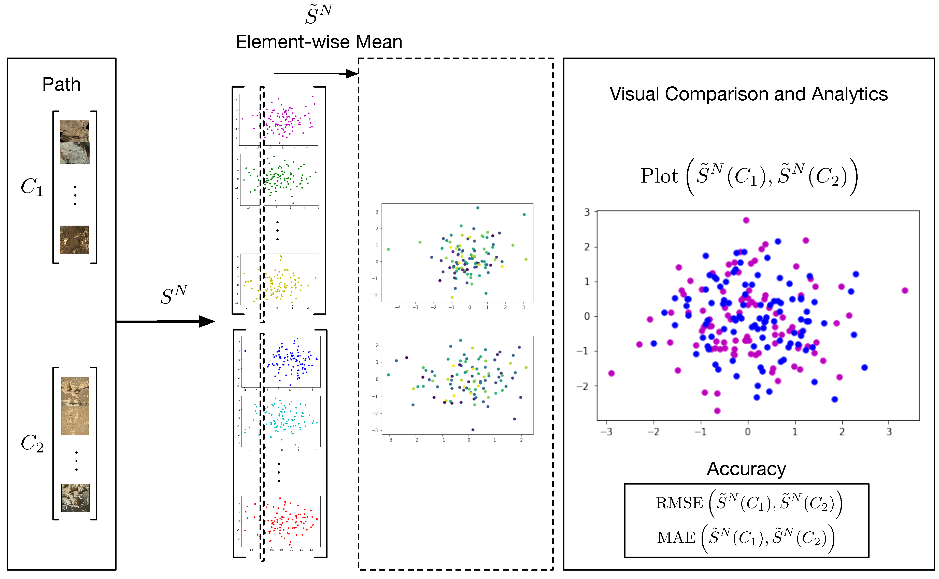
6.1. Statistical Analysis of the Generated Distribution
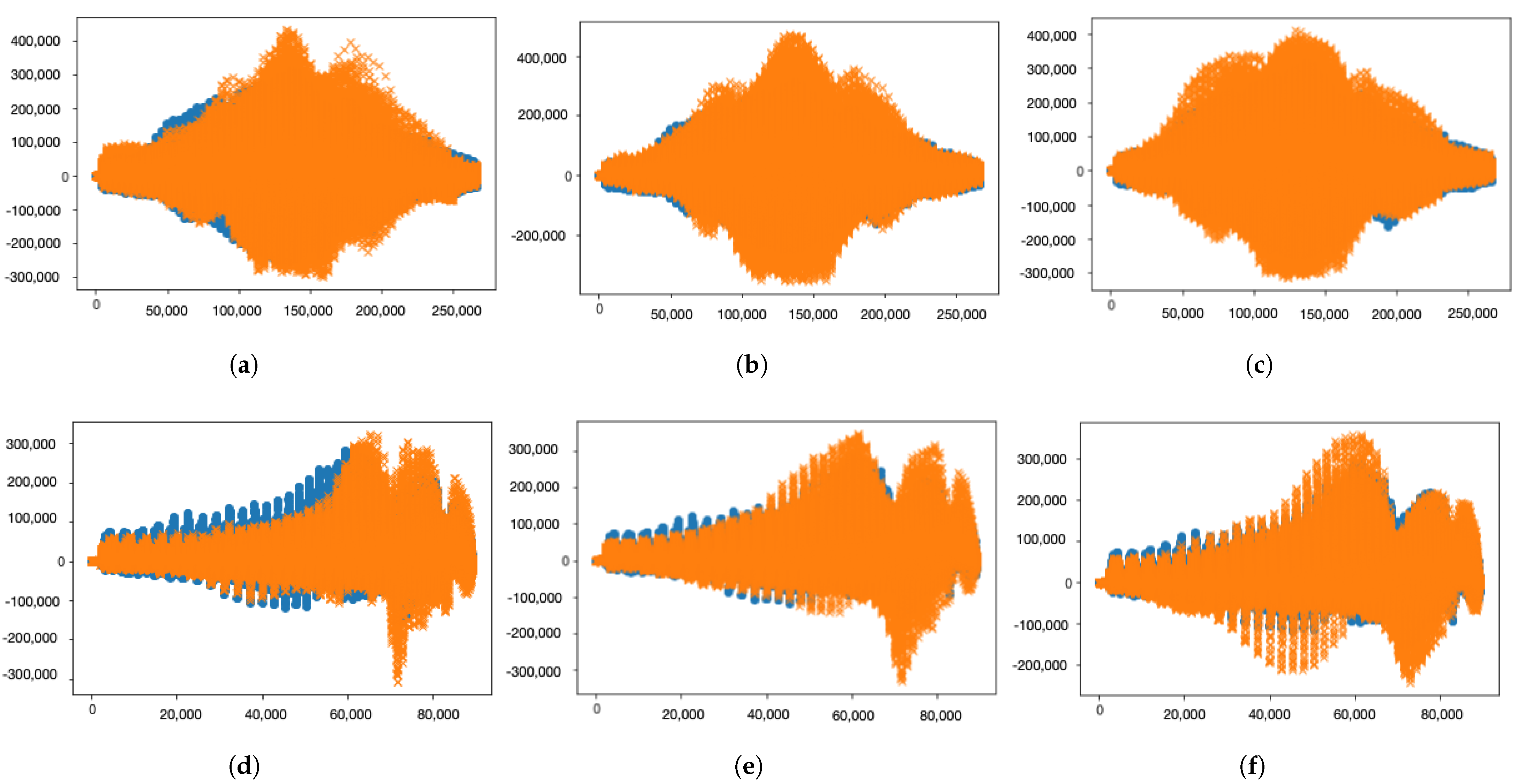
In this study, we perform a preliminary statistical analysis using Kruskal–Wallis [71] to evaluate the goodness of fit between the original and synthetic samples generated by GANs. We use the mean raster image intensities or gray-scale values as a simple image descriptor to capture rough texture information. Prior to conducting Kruskal–Wallis, we assess homoscedasticity using Levene’s test and normality of the distributions using a normality test, such as the Shapiro–Wilk test.
As a result of this preliminary analysis, we find that the original samples do not follow a normal distribution, whereas the synthetic samples do. This is consistent with the GAN architecture, which initially models the samples as White Gaussian and then modifies them to fit the original distribution. However, Kruskal–Wallis does not support the null hypothesis for goodness of fit, suggesting that a more sophisticated method for measuring sample quality in GANs is necessary. Existing measures such as MS-SSIM [37] and FID [8] are commonly used for this purpose. Despite its simplicity, the proposed non-parametric analysis can serve as a unit test for GANs and other variational methods after the model is trained, providing a quick assessment of the sample quality. This approach depicted in Figure 1 has not been extensively explored in the literature and offers a valuable contribution to the field.
Description and interpretation of statistical measures are provided in Table 1:
(a)
Necessary condition but not sufficient to assert that both populations originate from the same distribution.
(b)
There is not enough statistical evidence to attest both populations’ samples originate from the same distribution.
(c)
With high probability the synthetic distribution generated is still close enough to the initial distribution of noise from the GAN architecture. The samples may not show enough fidelity, and there is probably bad generalization behavior.
(d)
The synthetic distribution is far from the initial distribution of noise and has deviated from the original Normal, and may be close to the target distribution.
(e)
If (a) then there is enough statistical evidence to confirm that both populations originate from the same distribution given this image descriptor. If (a) is not fulfilled, then we can only ascertain that the synthetic population is a good approximation.
(f)
There is not enough statistical evidence to attest both populations are from the same distribution.
In Table 2, we present the evaluation test measures for homoscedasticity (T1), normality (T2), and goodness of fit (T3) on NASA Perseverance, AFHQ [72], and MetFaces [70] datasets. Based on the interpretation outlined in Table 1 and using the given image descriptor, we deduce that the Stylegan2-ada models trained on AFHQ Cat and Wild datasets provide excellent approximations of the original distributions, as the null hypothesis for goodness of fit is accepted. However, we cannot conclude that the distributions are identical since the equality of variances is not confirmed.
For the AFHQ Dog dataset, additional training is required as the null hypothesis for T2 (normality of the synthetic distribution) is accepted, indicating that the learned distribution is close to the original white noise. A similar conclusion applies to the model trained on the NASA Perseverance dataset, which also needs further training. In the case of MetFaces, the learned distribution is considerably different from the original white noise, but the null hypothesis for goodness of fit is not accepted. This finding suggests several possible interpretations: the model may be overfitting, it might require increased capacity to represent all features of the original distribution, or additional training might be needed.
We have introduced statistical measures and a visualization pipeline to examine and comprehend the data at hand. Nevertheless, the high-dimensional nature of images, coupled with the sequential aspect of video streams, brings forth a sense of time and space that our current analysis does not accommodate. In fact, the data comprise a series of images captured over a linear time span, following a specific trajectory. To address this aspect, we will employ tools from harmonic analysis in the subsequent section to offer a more comprehensive interpretation.

6.2. RMSE and MAE Signature and Log-Signature

The Signature Transform [10,73,74,75,76] is roughly equivalent to Fourier; instead of extracting information about frequency, it extracts information about order and area.
However, the Signature Transform differs from Fourier by the fact that it utilizes a basis of the space of functions of paths, a more general case to the basis of space of paths found in the preceding.
Following [10], the truncated signature of order N of the path x is defined as a collection of coordinate iterated integrals
S N ( x ) = 0 < t 1 < < t a < 1 c = 1 a d f z c d t ( t c ) d t 1 d t a 1 z 1 , , z a d 1 a N .
The Signature is a homomorphism from the monoid of paths into the grouplike elements of a closed tensor algebra; see Equation (16). It provides a graduated summary of the path x . These extracted features of a path are at the center of the definition of a rough path [14]; they remove the necessity to take into account the inner detailed structure of the path.
S : f F | f : [ x , y ] E = R d T ( E ) ,
where   T ( E ) = T ( R d ) = c = 0 R d c .
It has many advantages over other tools of harmonic analysis for ML. It is a universal non-linearity, which means that every continuous function of the input stream may be approximated arbitrarily by a linear function of its signature. Furthermore, among other properties, it presents outstanding robustness behavior to missing or irregularly sampled data, along with optional invariance in terms of translation and sampling. It has recently been introduced in the context of DL to add some structure to the learning process, and it seems a promising tool in Generative Models and Reinforcement Learning, as well as a good theoretical framework. It mainly works on streams of data which could describe from video sequences to our entire life experiences. That is to say, under the correct assumptions and the right application, it could potentially compress all human experiences into a representation that could be stored and processed efficiently. Here, we propose to conduct a preliminary study in terms of harmonic analysis and understand its properties to compare the original and synthetic samples.
The Signature [11,14,77,78,79,80] of an input data stream encodes the order in which data arrive without being concerned with the precise timing of its arrival. This property, known as invariance to time reparameterizations [81], makes it an ideal candidate for measuring GAN-generated distributions against an original data stream. Notably, when sampling the GAN model, instances of the latent space are retrieved in no specific order, even though the original data are inherently time-dependent, as recorded video streams or images captured by sensors are constrained by the temporal nature of the physical world. However, GANs are not yet capable of generating data linearly in time and space, making comparisons using other methods potentially biased or unable to capture all relevant cues.
Furthermore, it is essential to note that the number of components in the truncated signature does not depend on the number of data samples under consideration. Specifically, it maps the infinite-dimensional space of data streams, S ( R d ) , into a finite-dimensional space of dimension ( d N + 1 1 ) / ( d 1 ) , where N corresponds to the order of the truncated signature. This characteristic makes the Signature Transform highly suitable for processing long sequential data with varying lengths or unevenly sampled data.
At the same time, we can introduce the concept of Log-Signature [75,76], which is a more compact representation than the Signature.
Definition 1.
If γ t E is a path segment and S is its Signature, then
S = 1 + S 1 + S 2 + c , S c E c , log 1 + x = x x 2 / 2 + , log S = S 1 + S 2 + S 1 + S 2 + 2 / 2 +
The series log S = S 1 + S 2 + S 1 + S 2 + 2 / 2 + which is well-defined, is referred to as the Log-Signature of γ .
In practice, the Log-Signature calculation involves a series expansion that is typically truncated at a certain level to obtain a finite-dimensional representation. The choice of the truncation level depends on the specific application and the desired trade-off between computational complexity and the level of detail captured by the Log-Signature. In our experiments, we have chosen a truncation level that balances these considerations and yields satisfactory performance for our GAN evaluation task.
Unlike the Signature, the Log-Signature does not guarantee universality [14], and as a result, it needs to be combined with non-linear models for learning. However, it is empirically more robust to sparsely sampled data. There is a one-to-one correspondence between the Signature and the Log-Signature, as the logarithm map is bijective [13,75]. This statement also holds true for the truncated case up to the same degree.
In this study, we perform a comparison of the mean signature and Log-Signature for original and synthetic samples at a size of 64 × 64 . We observe that synthetic samples encompass the most relevant information from the original harmonic distribution. We compare against sets of 1000 and 5000 synthetic samples, with each instance considered a path x of dimension 64 to which we apply the Signature and Log-Signature transforms.
We propose the use of the element-wise mean of the truncated signatures S ˜ N , depicted in Figure 2, to analyze the convergence of GAN-learned models by employing RMSE (Root Mean Squared Error) and MAE (Mean Absolute Error). We refer to these measures as RMSE and MAE Signature, and RMSE and MAE Log-Signature. For instance, in Figure 3, we can observe that the model is achieving good convergence, though it is not capturing all the information present in the original distribution.
RMSE and MAE, when understood through the element-wise mean, can be considered as score functions built upon the Signature Transform, capable of measuring the quality of the generated distribution. This perspective on these measures is important for future applications, as it allows for the possibility of generalizing them to other tasks [11] or even applying them to other transforms. RMSE and MAE Signature and Log-Signature can serve multiple purposes, such as comparing models, monitoring performance during training across several epochs, and analytically detecting overfitting, as demonstrated in Table 3, whereas all these measures capture information about the visual cues present in the distributions, RMSE and MAE Signature, as well as MAE Log-Signature, prove to be more accurate in tracking the convergence of the GAN training procedure. In contrast, the RMSE Log-Signature exhibits less precision.
In Table 3, we present the RMSE and MAE Signature and Log-Signature values for different iterations of Stylegan2-ADA training. These values are calculated to evaluate the performance of the GAN at various stages of its training process. A closer examination of the table reveals that the 798th iteration of Stylegan2-ADA achieves the lowest RMSE and MAE Signature and Log-Signature values, which indicates the highest accuracy among the listed iterations. This table demonstrates the utility of RMSE and MAE Signature and Log-Signature metrics in tracking the progress of GAN training and identifying the optimal model iteration. By comparing the values across different iterations, we can observe the improvements in GAN performance as it learns to generate more realistic images. Furthermore, the table showcases the effectiveness of our proposed metrics in detecting potential overfitting, as evidenced by the increased RMSE and MAE values in the 983rd iteration. This increase in values suggests a decline in the GAN’s performance, likely due to overfitting the training data. In summary, Table 3 highlights the value of our proposed RMSE and MAE Signature and Log-Signature metrics in evaluating GAN performance, enabling us to monitor progress, compare different models, and detect overfitting during the training process.
To provide a more comprehensive understanding of the concepts presented in this section, we will analytically describe the abstraction of a set of images as an unevenly sampled stream of data, for example, a path, and present the definitions used to measure the similarity between image distributions.
A stream of data, x S ( R d ) , can be understood as a discrete representation of a path.
Definition 2.
Let x = ( x 1 , , x n ) S ( R d ) be a stream of data. Let X be a linear interpolation of x . Then the signature of x is defined as
S ( x ) = S ( X ) ,
and the truncated signature of order N of x is defined as
S N ( x ) = S N ( X ) .
This definition of the signature of a stream of data is independent of the choice of linear interpolation of X by the invariance to time reparameterizations [10].
Definition 3.
Given a set of truncated signatures of order N, S c N ( x c ) c = 1 m , the element-wise mean is defined by
S ˜ N ( x ( z ) ) = 1 m c = 1 m S c N ( x c ( z ) ) ,
where z { 1 , , n } is the specific component index of the given signature.
Then, RMSE and MAE Signature, whose results are presented in Table 3 and Table 4, can be defined as follows.
Definition 4.
Given n components of the element-wise mean of the signatures { y ˜ ( c ) } c = 1 n T ( R d ) from the model chosen as a source of synthetic samples and the same number of components of the element-wise mean of the signatures { x ˜ ( c ) } c = 1 n T ( R d ) from the original distribution, we define the Root Mean Squared Error (RMSE) and Mean Absolute Error (MAE) by
RMSE x ˜ ( c ) c = 1 n , y ˜ ( c ) c = 1 n = 1 n c = 1 n y ˜ ( c ) x ˜ ( c ) 2 ,
and
MAE x ˜ ( c ) c = 1 n , y ˜ ( c ) c = 1 n = 1 n c = 1 n | y ˜ ( c ) x ˜ ( c ) | .
The case for Log-Signature is analogous.

7. Evaluation

We present the results of our proposed measures using several state-of-the-art pretrained models in Table 4. For evaluation and testing, we use the standard AFHQ dataset [72] classes ‘cat’, ‘dog’, and ‘wild’, as well as MetFaces [70], in conjunction with their corresponding pretrained models. To compute the RMSE and MAE for S ˜ N and log S ˜ N , we generate 1000 synthetic samples from each model and compare them against the full original dataset. Prior to the Signature Transform, the samples are converted to grayscale and resized to 64 × 64 . Figure 4 and Figure 5 provide a visual comparison of the spectrum, demonstrating that the trained models effectively learn the empirical distribution of the original data.
The AFHQ dataset comprises high-quality images of animal faces, which are divided into three distinct classes: cats, dogs, and wildlife. This dataset provides a challenging evaluation scenario due to the inherent differences between the classes and the detailed textures present in the animal faces. MetFaces, on the other hand, is a collection of face images derived from various art pieces, including paintings, photographs, and sculptures. It showcases a diverse range of artistic styles, time periods, and image content, making it an ideal dataset to assess the performance of our proposed metrics on more complex and varied data distributions. By evaluating our method on both AFHQ and MetFaces, we aim to demonstrate the adaptability and robustness of our approach across different scenarios and data complexities.
In Table 4, we compare the recently developed models r , t -Stylegan3-ADA [43] against Stylegan2-ADA using MetFaces. We observe that t-Stylegan3-ADA significantly outperforms Stylegan2-ADA and r-Stylegan3-ADA, which is consistent with the FID results reported in [43], as shown in Table 5. Here, we can see that FID closely resembles the behavior of RMSE S ˜ 3 . Nonetheless, our metrics are both effective and efficient. A visual comparison of the spectrum of the Signatures for the given dataset can be seen in Figure 5. Computation is performed on the CPU in seconds, which is orders of magnitude faster and requires fewer resources than FID or MS-SSIM.
Table 4 presents the RMSE and MAE Signature and Log-Signature evaluation results for different GAN models and datasets, including AFHQ and MetFaces. The table showcases a comparison of state-of-the-art pretrained models: Stylegan2-ADA [70], r-Stylegan3-ADA, and t-Stylegan3-ADA [43]. The goal of this comparison is to highlight the performance differences between these models using the proposed metrics. A close inspection of the table reveals that the t-Stylegan3-ADA model consistently achieves the lowest RMSE and MAE Signature and Log-Signature values across all datasets, indicating superior performance in generating synthetic samples that closely resemble the original distributions. This result demonstrates the effectiveness of the t-Stylegan3-ADA model in learning the intricacies of the underlying data distributions and generating high-quality synthetic samples. Additionally, the table illustrates the performance variations between different categories within the AFHQ dataset, with AFHQ Cat and Wild categories having a closer resemblance to the original distributions than AFHQ Dog. This observation aligns with the qualitative assessment of the generated samples visualized in Figure 6 and Figure 7, providing further evidence of the accuracy of our proposed metrics in capturing the characteristics of the generated samples. That is, Table 4 highlights the utility of the RMSE and MAE Signature and Log-Signature metrics in evaluating and comparing the performance of different GAN models across various datasets. By analyzing these metrics, we can gain insights into the quality of the generated samples and their similarity to the original distributions, as well as assess the effectiveness of the GAN models in capturing the essential features of the data.
Table 5 presents a comparison of the FID and RMSE S ˜ 3 metrics on MetFaces for three GAN models: Stylegan2-ADA, r-Stylegan3-ADA, and t-Stylegan3-ADA. The aim of this comparison is to highlight the relationship between the two evaluation metrics and demonstrate the efficacy of RMSE S ˜ 3 in capturing the performance differences among these models. As observed in the table, the FID scores and RMSE S ˜ 3 values show a similar trend, with t-Stylegan3-ADA achieving the best performance in both metrics. This consistency between the two evaluation metrics suggests that RMSE S ˜ 3 can serve as a reliable alternative to FID in assessing GAN performance. Moreover, the lower RMSE S ˜ 3 values for t-Stylegan3-ADA indicate that the model generates synthetic samples that are closer to the original distribution compared to the other two models. Notably, the proposed RMSE S ˜ 3 metric offers significant advantages over FID in terms of computational efficiency and resource requirements. As mentioned in the text, the RMSE S ˜ 3 computations are performed on the CPU in seconds, making it substantially faster and less resource-intensive than FID or MS-SSIM. This efficiency makes the proposed metric more suitable for practical applications, where rapid evaluation and limited resources may be critical factors. In summary, Table 5 demonstrates the effectiveness of the RMSE S ˜ 3 metric as an alternative to FID for evaluating GAN performance. The strong correlation between the two metrics, coupled with the computational advantages of RMSE S ˜ 3 , showcases its potential as a valuable tool for assessing the quality of synthetic samples generated by various GAN models.

7.1. Computational Complexity

In this subsection, we elaborate on the computational complexity and time estimates for the element-wise mean of the Signatures and Kruskal–Wallis in comparison to FID, MS-SSIM, LPIPS, and PSNR.
  • Element-wise mean of the Signatures: The computation of the Signature Transform has a time complexity of O ( L M 2 ) , where L is the length of the path and M is the order of the signature. However, since we are computing the element-wise mean of the Signatures, the complexity becomes O ( N L M 2 ) , where N is the number of samples. In practice, the Signature Transform can be efficiently computed using recursive algorithms, which keeps the computational cost low.
  • Kruskal–Wallis has a time complexity of O ( N log N ) for sorting the samples, followed by O ( N ) for computing the test statistic, resulting in an overall complexity of O ( N log N ) . This complexity is relatively low, especially when compared to more computationally demanding metrics such as FID and MS-SSIM.
In comparison:
  • The FID calculation involves computing the Inception features for each sample, which requires a forward pass through a deep neural network, followed by computing the mean and covariance of these features. The complexity of the forward pass depends on the architecture of the Inception network, but it is generally much higher than the complexity of the Signature Transform and the Kruskal–Wallis. Additionally, FID requires GPU resources to perform these calculations efficiently, further increasing its computational cost.
  • MS-SSIM involves computing the structural similarity index at multiple scales, which requires computing the mean, variance, and covariance for each scale. The complexity of MS-SSIM is O ( N W H ) , where W and H are the width and height of the images, respectively, whereas this complexity is not as high as FID, it is still higher than the complexities of the proposed methods.
  • LPIPS metric computes the distance between image features extracted from a pretrained deep neural network (e.g., AlexNet or VGG). The complexity of LPIPS is primarily determined by the forward pass through the chosen deep neural network. The complexity of the forward pass depends on the architecture of the network, but in general, it is higher than the complexity of the Signature Transform and the Kruskal–Wallis. Similar to FID, LPIPS also typically requires GPU resources for efficient computation.
  • PSNR is a simple and widely used metric for image quality assessment. It is computed as the ratio between the maximum possible power of a signal and the power of corrupting noise that affects the fidelity of its representation. The complexity of PSNR is O ( N W H ) , where W and H are the width and height of the images, respectively. Although the complexity of PSNR is similar to that of MS-SSIM, it is still higher than the complexities of the proposed methods (element-wise mean of the Signatures and Kruskal–Wallis).
To summarize, our proposed methods (element-wise mean of the Signatures and Kruskal–Wallis) have significantly lower computational complexity than FID, MS-SSIM, LPIPS, and PSNR, allowing for faster computation and reduced resource usage. Based on the complexity analysis, we can estimate that our methods can be computed on the CPU in seconds, whereas FID, MS-SSIM, LPIPS, and PSNR require more time and resources, particularly when GPUs are not available.

7.2. Visualization

In our study, we first apply PCA to reduce the dimensionality of the data, which helps us to retain the global structure of the dataset. Then, we use t-SNE to visualize the data in a lower-dimensional space, which emphasizes the local differences between samples. This two-step approach allows us to capture both the global and local structures within the data, providing a richer visualization of the generated GAN images compared to using PCA alone.
In Figure 6 and Figure 7, we visualize the sets of images of AFHQ and MetFaces, both original and synthetic, used in the evaluations in Table 2 and Table 4 using PCA Adaptive t-SNE. The importance here is to observe the overall distribution of the samples, which is well captured by our proposed method. For instance, we can observe that the synthetic samples of AFHQ Cat and Wild closely resemble the original distribution in terms of variability and quality. In contrast, AFHQ Dog demonstrates less variability but still achieves high-quality samples, which aligns with the analytical interpretation of the proposed statistical measures shown in Table 2.
In Figure 7, we can observe that the synthetic samples generated with t-Stylegan3-ADA exhibit better quality than those produced by Stylegan2-ADA and r-Stylegan3-ADA, and the model is evidently learning the original distribution. Nonetheless, there is potential for improvement in terms of variability and scope. These observations are consistent with the RMSE and MAE Signature and Log-Signature results, as shown in Table 4.
That being said, our proposed method relies on the Signature Transform and Log-Signature to evaluate GAN-generated samples, which are independent of PCA and t-SNE. The use of PCA and t-SNE in our study is only to provide a visual representation of the original and synthetic distributions, allowing us to better understand and interpret the quality of the generated images. The sample size and analysis time of the generated GAN images are not affected by the application of PCA and t-SNE for visualization. Our methodology remains efficient and effective in assessing the quality of GAN-generated samples without the need to reduce the dimensionality of the images for the actual evaluation process.

8. Conclusions

GAN evaluation has been one of the central research efforts of the community of computer vision during these last years. The ability of the networks to generate high-fidelity samples has inspired researchers all over the world to work on the topic. However, although many variants of the original successful DCGAN architecture are able to generate very realistic samples, neither the advance in proposing metrics to assess the imagery has been effectual, nor the ability of the metrics to guarantee some level of robustness, and overall description of the resultant distribution. The best effort of them being FID suffers from high-computation time and use of GPU resources; it depends mainly on an inception module that extracts features from lots of samples rather than from analytical measures that quantify properly their characteristics.
We are the first to propose the use of the Signature Transform to assess GAN convergence by introducing RMSE and MAE Signature and Log-Signature. The measures are reliable, consistent, efficient, and easy to compute. Additionally, an effective methodology to test the goodness-of-fit according to the original distribution by the use of simple statistical methods is also proposed, being the first to be able to reduce the amount of computation for accurate GAN Synthetic image quality assessment to the order of seconds. Worth mentioning is the proposal of a taxonomical pipeline to systematically assess the resultant distributions using a non-parametric test. Lastly, we also introduce an adaptive technique based on t-SNE and PCA that, without the need for hyperparameter tuning, puts forward exceptional visualization capabilities.
Future work that could be pursued under these assumptions, among others, is to increase the complexity of the descriptor, extend the proposed score functions on top of the Signature Transform to be used in other tasks or use the metrics inside the training loop to assess convergence and help the networks train faster.
In this study, we presented a novel approach to assess GAN convergence and goodness of fit using the Signature Transform, whereas our methodology provides significant advantages over existing methods, we acknowledge the following limitations:
  • The proposed RMSE and MAE Signature and Log-Signature metrics are based on the Signature Transform, which inherently captures information about the underlying distribution. However, these metrics may not be sensitive to certain aspects of the generated images, such as fine-grained details or specific structures, which could be essential for certain applications.
  • Although our proposed method significantly reduces computation time and resource usage compared to existing GAN evaluation methods, it might still be computationally expensive for extremely large datasets or high-resolution images. Further optimization of the computation process may be necessary to address these challenges.
  • The evaluation of GAN performance based on our proposed metrics assumes that the original and synthetic image distributions are stationary. In cases where the data exhibit non-stationary behavior, the effectiveness of our approach might be compromised, and additional methods or adaptations may be required.
  • The goodness-of-fit methodology proposed in this study relies on statistical methods, which might not always provide definitive conclusions on the quality of the generated samples. In some cases, additional qualitative assessments or domain-specific evaluations may be necessary to obtain a comprehensive understanding of the GAN’s performance.
In conclusion, despite these limitations, our study introduces a promising and efficient approach to assess GAN convergence and goodness of fit using the Signature Transform. Future work may involve addressing these limitations and further exploring the potential of our proposed metrics in other applications and tasks.

Author Contributions

Conceptualization, J.d.C. and I.d.Z.; funding acquisition, C.T.C. and G.R.; investigation, J.d.C. and I.d.Z.; methodology, J.d.C. and I.d.Z.; software, J.d.C. and I.d.Z.; supervision, G.R. and C.T.C.; writing—original draft, J.d.C.; writing—review and editing, C.T.C., G.R., J.d.C. and I.d.Z. All authors have read and agreed to the published version of the manuscript.

Funding

This work was supported by the HK Innovation and Technology Commission (InnoHK Project CIMDA). We acknowledge the support of R&D project PID2021-122580NB-I00, funded by MCIN/AEI/10.13039/501100011033 and ERDF. We thank the following funding sources from GOETHE-University Frankfurt am Main; ‘DePP—Dezentrale Plannung von Platoons im Straßengüterverkehr mit Hilfe einer KI auf Basis einzelner LKW’ and ‘Center for Data Science & AI’.

Institutional Review Board Statement

Not applicable.

Informed Consent Statement

Not applicable.

Data Availability Statement

Not applicable.

Conflicts of Interest

The authors declare that they have no conflict of interest. The funders had no role in the design of the study, in the collection, analyses, or interpretation of data, in the writing of the manuscript, or in the decision to publish the results.

Abbreviations

The following abbreviations are used in this manuscript:
DNNDeep Neural Networks
DLDeep Learning
MLMachine Learning
NLPNatural Language Processing
RMSERoot Mean Squared Error
MAEMean Absolute Error
GANGenerative Adversarial Networks
ADAAdaptive Discriminator Augmentation
FIDFréchet Inception Distance
MS-SSIMStructural Similarity Index Measure
LPIPSLearned Perceptual Image Patch Similarity
PSNRPeak Signal-to-Noise Ratio
PCAPrincipal Component Analysis
KLKullback–Leibler
GPUGraphics Processing Unit
t-SNEt-Distributed Stochastic Neighbor Embedding

References

  1. Goodfellow, I.; Pouget-Abadie, J.; Mirza, M.; Xu, B.; Warde-Farley, D.; Ozair, S.; Courville, A.; Bengio, Y. Generative adversarial networks. In Proceedings of the Annual Conference on Neural Information Processing Systems, Montreal, QC, Canada, 8–13 December 2014; Volume 27. [Google Scholar]
  2. Isola, P.; Zhu, J.-Y.; Zhou, T.; Efros, A.A. Image-to-Image Translation with Conditional Adversarial Networks. In Proceedings of the IEEE Conference on Computer Vision and Pattern Recognition (CVPR), Honolulu, HI, USA, 21–26 July 2017; pp. 1125–1134. [Google Scholar]
  3. Kang, M.; Zhu, J.-Y.; Zhang, R.; Park, J.; Shechtman, E.; Paris, S.; Park, T. Scaling up GANs for Text-to-Image Synthesis. arXiv 2023, arXiv:2303.05511. [Google Scholar]
  4. Karras, T.; Laine, S.; Aila, T. A style-based generator architecture for generative adversarial networks. IEEE Trans. Pattern Anal. Mach. Intell. 2019, 43, 4217–4228. [Google Scholar] [CrossRef]
  5. Chan, E.R.; Lin, C.Z.; Chan, M.A.; Nagano, K.; Pan, B.; Mello, S.D.; Gallo, O.; Guibas, L.J.; Tremblay, J.; Khamis, S.; et al. Efficient geometry-aware 3D generative adversarial networks. In Proceedings of the IEEE/CVF Conference on Computer Vision and Pattern Recognition, New Orleans, LA, USA, 18–24 June 2022; pp. 16123–16133. [Google Scholar]
  6. Brock, A.; Donahue, J.; Simonyan, K. Large scale gan training for high fidelity natural image synthesis. In Proceedings of the 35th International Conference on Machine Learning, Stockholm, Sweden, 10–15 July 2019. [Google Scholar]
  7. Zhao, L.; Zhang, Z.; Chen, T.; Metaxas, D.N.; Zhang, H. Improved transformer for high-resolution gans. In Proceedings of the Annual Conference on Neural Information Processing Systems NIPS, Virtual, 6–14 December 2021. [Google Scholar]
  8. Heusel, M.; Ramsauer, H.; Unterthiner, T.; Nessler, B.; Hochreiter, S. GANs trained by a two time-scale update rule converge to a local nash equilibrium. In Proceedings of the Annual Conference on Neural Information Processing Systems 2017, Long Beach, CA, USA, 4–9 December 2017; Volume 30. [Google Scholar]
  9. Wang, Z.; Bovik, A.C.; Sheikh, H.R.; Simoncelli, E.P. Multiscale structural similarity for image quality assessment. In Proceedings of the Thrity-Seventh Asilomar Conference on Signals, Systems & Computers, Pacific Grove, CA, USA, 9–12 November; 2003; Volume 2, pp. 1398–1402. [Google Scholar]
  10. Bonnier, P.; Kidger, P.; Arribas, I.P.; Salvi, C.; Lyons, T. Deep signature transforms. In Proceedings of the Annual Conference on Neural Information Processing Systems NIPS, Vancouver, BC, Canada, 8–14 December 2019. [Google Scholar]
  11. de Curtò, J.; de Zarzà, I.; Roig, G.; Calafate, C.T. Summarization of Videos with the Signature Transform. Electronics 2023, 12, 1735. [Google Scholar] [CrossRef]
  12. Chen, K.-T. Iterated path integrals. Bull. Am. Math. Soc. 1977, 83, 831–879. [Google Scholar] [CrossRef]
  13. Lyons, T.; Caruana, M.; Levin, T. Differential Equations Driven by Rough Paths, Proceedings of the 34th Summer School on Probability Theory, Saint-Flour, France, 6–24 July 2004; Springer: Berlin/Heidelberg, Germany, 2007. [Google Scholar]
  14. Lyons, T. Rough paths, signatures and the modelling of functions on streams. In Proceedings of the International Congress of Mathematicians, Madrid, Spain, 22–30 August 2014. [Google Scholar]
  15. van der Maaten, L.; Hinton, G. Visualizing data using t-SNE. JMLR 2008, 9, 2579–2605. [Google Scholar]
  16. Girshick, R.; Donahue, J.; Darrell, T.; Malik, J. Rich feature hierarchies for accurate object detection and semantic segmentation. In Proceedings of the IEEE Conference on Computer Vision and Pattern Recognition, Columbus, OH, USA, 23–28 June 2014. [Google Scholar]
  17. He, K.; Zhang, X.; Ren, S.; Sun, J. Delving deep into rectifiers: Surpassing human-level performance on ImageNet classification. In Proceedings of the IEEE International Conference on Computer Vision (ICCV), Santiago, Chile, 7–13 December 2015. [Google Scholar]
  18. Girshick, R. Fast R-CNN. In Proceedings of the IEEE International Conference on Computer Vision (ICCV), Santiago, Chile, 7–13 December 2015. [Google Scholar]
  19. Chen, L.; Papandreou, G.; Kokkinos, I.; Murphy, K.; Yuille, A.L. DeepLab: Semantic Image Segmentation with Deep Convolutional Nets, Atrous Convolution, and Fully Connected CRFs. IEEE Trans. Pattern Anal. Mach. Intell. 2017, 40, 834–848. [Google Scholar] [CrossRef]
  20. Chen, Q.; Koltun, V. Photographic image synthesis with cascaded refinement networks. In Proceedings of the IEEE International Conference on Computer Vision (ICCV), Venice, Italy, 22–29 October 2017. [Google Scholar]
  21. Yang, B.; Luo, W.; Urtasun, R. PIXOR: Real-time 3D object detection from point clouds. In Proceedings of the IEEE Conference on Computer Vision and Pattern Recognition, Salt Lake City, UT, USA, 18–23 June 2018. [Google Scholar]
  22. Parmar, N.; Vaswani, A.; Uszkoreit, J.; Kaiser, L.; Shazeer, N.; Ku, A.; Tran, D. Image transformer. In Proceedings of the 35th International Conference on Machine Learning, ICML, Stockholm, Sweden, 10–15 July 2018. [Google Scholar]
  23. Mildenhall, B.; Srinivasan, P.P.; Tancik, M.; Barron, J.T.; Ramamoorthi, R.; Ng, R. NeRF: Representing scenes as neural radiance fields for view synthesis. In Proceedings of the ECCV 2020: 16th European Conference, Glasgow, UK, 23–28 August 2020. [Google Scholar]
  24. Park, T.; Efros, A.A.; Zhang, R.; Zhu, J. Contrastive learning for unpaired image-to-image translation. In Proceedings of the ECCV 2020: 16th European Conference, Glasgow, UK, 23–28 August 2020. [Google Scholar]
  25. Long, J.; Shelhamer, E.; Darrell, T. Fully convolutional networks for semantic segmentation. In Proceedings of the IEEE Conference on Computer Vision and Pattern Recognition, Boston, MA, USA, 7–12 June 2015. [Google Scholar]
  26. Redmon, J.; Divvala, S.; Girshick, R.; Farhadi, A. You only look once: Unified, real-time object detection. In Proceedings of the IEEE Conference on Computer Vision and Pattern Recognition, Las Vegas, NV, USA, 27–30 June 2016. [Google Scholar]
  27. Gatys, L.A.; Ecker, A.S.; Bethge, M. Image style transfer using convolutional neural networks. In Proceedings of the IEEE International Conference on Computer Vision, Las Vegas, NV, USA, 27–30 June 2016. [Google Scholar]
  28. Gatys, L.A.; Bethge, M.; Hertzmann, A.; Shechtman, E. Preserving color in neural artistic style transfer. arXiv 2016, arXiv:1606.05897. [Google Scholar]
  29. Karras, T.; Aila, T.; Laine, S.; Lehtinen, J. Progressive growing of GANs for improved quality, stability, and variation. In Proceedings of the 6th ICLR International Conference on Learning Representations, Vancouver, BC, Canada, 30 April–3 May 2018. [Google Scholar]
  30. He, K.; Gkioxari, G.; Dollár, P.; Girshick, R. Mask R-CNN. In Proceedings of the IEEE International Conference on Computer Vision, Venice, Italy, 22–29 October 2017. [Google Scholar]
  31. Vaswani, A.; Shazeer, N.; Parmar, N.; Uszkoreit, J.; Jones, L.; Gomez, A.N.; Kaiser, L.; Polosukhin, I. Attention is all you need. In Proceedings of the Annual Conference on Neural Information Processing Systems, Long Beach, CA, USA, 4–9 December 2017. [Google Scholar]
  32. Wang, T.; Liu, M.; Zhu, J.; Liu, G.; Tao, A.; Kautz, J.; Catanzaro, B. Video-to-video synthesis. In Proceedings of the Annual Conference on Neural Information Processing Systems, NeurIPS, Montréal, QC, Canada, 3–8 December 2018. [Google Scholar]
  33. de Zarzà, I.; de Curtò, J.; Calafate, C.T. Detection of glaucoma using three-stage training with EfficientNet. Intell. Syst. Appl. 2022, 16, 200140. [Google Scholar] [CrossRef]
  34. de Curtò, J.; de Zarzà, I.; Calafate, C.T. Semantic scene understanding with large language models on unmanned aerial vehicles. Drones 2023, 7, 114. [Google Scholar] [CrossRef]
  35. Dosovitskiy, A.; Brox, T. Generating Images with Perceptual Similarity Metrics Based on Deep Networks. In Proceedings of the 30th International Conference on Neural Information Processing Systems, Barcelona, Spain, 5–10 December 2017; pp. 658–666. [Google Scholar]
  36. Ratner, A.; Sa, C.D.; Wu, S.; Selsam, D.; Ré, C. Data Programming: Creating Large Training Sets, Quickly. In Proceedings of the 30th International Conference on Neural Information Processing Systems, Barcelona, Spain, 5–10 December 2017; pp. 3567–3575. [Google Scholar]
  37. Odena, A.; Olah, C.; Shlens, J. Conditional image synthesis with auxiliary classifier gans. In Proceedings of the CML’17: 34th International Conference on Machine Learning, Sydney, NSW, Australia, 6–11 August 2017. [Google Scholar]
  38. Antoniou, A.; Storkey, A.; Edwards, H. Data augmentation generative adversarial networks. In Proceedings of the 6th International Conference on Learning Representations, Vancouver, BC, Canada, 30 April–3 May 2018. [Google Scholar]
  39. Salimans, T.; Goodfellow, I.; Zaremba, W.; Cheung, V.; Radford, A.; Chen, X. Improved techniques for training GANs. In Proceedings of the Annual Conference on Neural Information Processing Systems, Barcelona, Spain, 5–10 December 2016. [Google Scholar]
  40. Mescheder, L.; Nowozin, S.; Geiger, A. The numerics of GANs. In Proceedings of the Annual Conference on Neural Information Processing Systems, Long Beach, CA, USA, 4–9 December 2017. [Google Scholar]
  41. Mescheder, L.; Geiger, A.; Nowozin, S. Which training methods for GANs do actually converge? In Proceedings of the International Conference on Machine Learning PMLR, Beijing, China, 14–16 November 2018. [Google Scholar]
  42. Jolicoeur-Martineau, A. The relativistic discriminator: A key element missing from standard GAN. In Proceedings of the 7th International Conference on Learning Representations, ICLR, New Orleans, LA, USA, 6–9 May 2019. [Google Scholar]
  43. Karras, T.; Aittala, M.; Laine, S.; Härkönen, E.; Hellsten, J.; Lehtinen, J.; Aila, T. Alias-free generative adversarial networks. In Proceedings of the Annual Conference on Neural Information Processing Systems NIPS, Virtual, 6–14 December 2021. [Google Scholar]
  44. Kingma, D.P.; Welling, M. Auto-encoding variational bayes. arXiv 2014, arXiv:1312.6114. [Google Scholar]
  45. Zhao, J.; Mathieu, M.; LeCun, Y. Energy-based generative adversarial networks. In Proceedings of the 5th International Conference on Learning Representations ICLR, Toulon, France, 24–26 April 2017. [Google Scholar]
  46. Wei, X.; Gong, B.; Liu, Z.; Lu, W.; Wang, L. Improving the improved training of wasserstein gans: A consistency term and its dual effect. In Proceedings of the 6th International Conference on Learning Representations ICLR, Vancouver, BC, Canada, 30 April–3 May 2018. [Google Scholar]
  47. Arora, S.; Ge, R.; Liang, Y.; Ma, T.; Zhang, Y. Generalization and Equilibrium in Generative Adversarial Nets (GANs). In Proceedings of the 34th International Conference on Machine Learning, PMLR, Seoul, Republic of Korea, 15–17 November 2017; pp. 224–232. [Google Scholar]
  48. Pascanu, R.; Mikolov, T.; Bengio, Y. On the Difficulty of Training Recurrent Neural Networks. In Proceedings of the 30th International Conference on Machine Learning, Atlanta GA, USA, 16–21 June 2013; pp. 1310–1318. [Google Scholar]
  49. Flynn, J.; Neulander, I.; Philbin, J.; Snavely, N. DeepStereo: Learning to Predict New Views from the World’s Imagery. In Proceedings of the IEEE Conference on Computer Vision and Pattern Recognition, Las Vegas, NV, USA, 27–30 June 2016; pp. 5515–5524. [Google Scholar]
  50. Song, Y.; Ermon, S. Generative modeling by estimating gradients of the data distribution. In Proceedings of the Annual Conference on Neural Information Processing Systems NIPS, Vancouver, BC, Canada, 8–14 December 2019. [Google Scholar]
  51. Roberts, G.O.; Tweedie, R.L. Exponential convergence of Langevin distributions and their discrete approximations. Bernoulli 1996, 2, 341–363. [Google Scholar] [CrossRef]
  52. Welling, M.; Teh, Y.W. Bayesian learning via stochastic gradient langevin dynamics. In Proceedings of the 28th International Conference on Machine Learning ICML, Bellevue, WA, USA, 28 June–2 July 2011. [Google Scholar]
  53. Song, Y.; Ermon, S. Improved techniques for training score-based generative models. In Proceedings of the Annual Conference on Neural Information Processing Systems NIPS, Virtual, 6–12 December 2020. [Google Scholar]
  54. Goyal, A.; Ke, N.R.; Ganguli, S.; Bengio, Y. Variational walkback: Learning a transition operator as a stochastic recurrent net. In Proceedings of the Annual Conference on Neural Information Processing Systems NIPS, Long Beach, CA, USA, 4–9 December 2017. [Google Scholar]
  55. Ho, J.; Jain, A.; Abbeel, P. Denoising diffusion probabilistic models. In Proceedings of the Annual Conference on Neural Information Processing Systems NIPS, Virtual, 6–12 December 2020. [Google Scholar]
  56. Jolicoeur-Martineau, A.; Piché-Taillefer, R.; Combes, R.T.; Mitliagkas, I. Adversarial score matching and improved sampling for image generation. In Proceedings of the International Conference on Learning Representations ICLR, Vienna, Austria, 4 May 2021. [Google Scholar]
  57. Zhao, Z.; Kunar, A.; Birke, R.; Chen, L.Y. Ctab-gan: Effective table data synthesizing. In Proceedings of the Machine Learning in Computational Biology Meeting, PMLR, Online, 22–23 November 2021; pp. 97–112. [Google Scholar]
  58. Dosovitskiy, A.; Beyer, L.; Kolesnikov, A.; Weissenborn, D.; Zhai, X.; Unterthiner, T.; Dehghani, M.; Minderer, M.; Heigold, G.; Gelly, S.; et al. An image is worth 16 × 16 words: Transformers for image recognition at scale. In Proceedings of the International Conference on Learning Representations ICLR, Addis Ababa, Ethiopia, 26–30 April 2020. [Google Scholar]
  59. Dhariwal, P.; Nichol, A. Diffusion models beat gans on image synthesis. Adv. Neural Inf. Process. Syst. 2021, 34, 8780–8794. [Google Scholar]
  60. Saharia, C.; Chan, W.; Chang, H.; Lee, C.; Ho, J.; Salimans, T.; Fleet, D.; Norouzi, M. Palette: Image-to-image diffusion models. In Proceedings of the ACM SIGGRAPH 2022, Vancouver, BC, Canada, 7–11 August 2022; pp. 1–10. [Google Scholar]
  61. Ulyanov, D.; Vedaldi, A.; Lempitsky, V. Deep image prior. In Proceedings of the IEEE/CVF Conference on Computer Vision and Pattern Recognition, Salt Lake City, UT, USA, 18–23 June 2018; pp. 9446–9454. [Google Scholar]
  62. Sohl-Dickstein, J.; Weiss, E.A.; Maheswaranathan, N.; Ganguli, S. Deep unsupervised learning using nonequilibrium thermodynamics. In Proceedings of the 7th Asian Conference on Machine Learning, Hong Kong, China, 20–22 November 2015; pp. 2256–2265. [Google Scholar]
  63. Vincent, P.; Larochelle, H.; Lajoie, I.; Bengio, Y.; Manzagol, P.-A. Stacked denoising autoencoders: Learning useful representations in a deep network with a local denoising criterion. J. Mach. Learn. Res. 2010, 11, 3371–3408. [Google Scholar]
  64. Ho, J.; Saharia, C.; Chan, W.; Fleet, D.J.; Norouzi, M.; Salimans, T. Cascaded Diffusion Models for High Fidelity Image Generation. J. Mach. Learn. Res. 2022, 23, 1–33. [Google Scholar]
  65. Luo, Z.; Chen, D.; Zhang, Y.; Huang, Y.; Wang, L.; Shen, Y.; Zhao, D.; Zhou, J.; Tan, T. VideoFusion: Decomposed Diffusion Models for High-Quality Video Generation. In Proceedings of the IEEE/CVF Conference on Computer Vision and Pattern Recognition (CVPR), Vancouver, BC, Canada, 20–22 June 2023. [Google Scholar]
  66. Wu, J.Z.; Ge, Y.; Wang, X.; Lei, S.W.; Gu, Y.; Hsu, W.; Shan, Y.; Qie, X.; Shou, M.Z. Tune-A-Video: One-Shot Tuning of Image Diffusion Models for Text-to-Video Generation. arXiv 2022, arXiv:2212.11565. [Google Scholar]
  67. Ruiz, N.; Li, Y.; Jampani, V.; Pritch, Y.; Rubinstein, M.; Aberman, K. Dreambooth: Fine tuning text-to-image diffusion models for subject-driven generation. arXiv 2022, arXiv:2208.12242. [Google Scholar]
  68. Hua, T.; Tian, Y.; Ren, S.; Zhao, H.; Sigal, L. Self-supervision through random segments with autoregressive coding (randsac). arXiv 2022, arXiv:2203.12054. [Google Scholar]
  69. Zhang, R.; Isola, P.; Efros, A.A.; Shechtman, E.; Wang, O. The unreasonable effectiveness of deep features as a perceptual metric. In Proceedings of the IEEE/CVF Conference on Computer Vision and Pattern Recognition, Salt Lake City, UT, USA, 18–23 June 2018; pp. 586–595. [Google Scholar]
  70. Karras, T.; Aittala, M.; Hellsten, J.; Laine, S.; Lehtinen, J.; Aila, T. Training generative adversarial networks with limited data. In Proceedings of the Annual Conference on Neural Information Processing Systems NIPS, Virtual, 6–12 December 2020. [Google Scholar]
  71. Kruskal, W.H.; Wallis, W.A. Use of ranks in one-criterion variance analysis. J. Am. Stat. Assoc. 1952, 47, 583–621. [Google Scholar] [CrossRef]
  72. Choi, Y.; Uh, Y.; Yoo, J.; Ha, J. Stargan v2: Diverse image synthesis for multiple domains. In Proceedings of the IEEE/CVF Conference on Computer Vision and Pattern Recognition (CVPR), Seattle, WA, USA, 13–19 June 2020. [Google Scholar]
  73. Kidger, P.; Lyons, T. Signatory: Differentiable computations of the signature and logsignature transforms, on both CPU and GPU. In Proceedings of the International Conference on Learning Representations ICLR, Vienna, Austria, 4 May 2021. [Google Scholar]
  74. Chevyrev, I.; Kormilitzin, A. A primer on the signature method in machine learning. arXiv 2016, arXiv:1603.03788. [Google Scholar]
  75. Liao, S.; Lyons, T.J.; Yang, W.; Ni, H. Learning stochastic differential equations using RNN with log signature features. arXiv 2019, arXiv:1908.08286. [Google Scholar]
  76. Morrill, J.; Kidger, P.; Salvi, C.; Foster, J.; Lyons, T.J. Neural CDEs for long time series via the log-ode method. In Proceedings of the 38th International Conference on Machine Learning ICML, Virtual, 18–24 July 2021. [Google Scholar]
  77. Kiraly, F.J.; Oberhauser, H. Kernels for sequentially ordered data. J. Mach. Learn. Res. 2019, 20, 1–45. [Google Scholar]
  78. Graham, B. Sparse arrays of signatures for online character recognition. arXiv 2013, arXiv:1308.0371. [Google Scholar]
  79. Chang, J.; Lyons, T. Insertion algorithm for inverting the signature of a path. arXiv 2019, arXiv:1907.08423. [Google Scholar]
  80. Fermanian, A. Learning Time-Dependent Data with the Signature Transform. Ph.D. Thesis, Sorbonne Université, Paris, France, 2021. Available online: https://tel.archives-ouvertes.fr/tel-03507274 (accessed on 1 November 2022).
  81. Lyons, T. Differential equations driven by rough signals. Rev. Mat. Iberoam. 1998, 14, 215–310. [Google Scholar] [CrossRef]
Figure 1. An illustrative representation of the proposed pipeline for the evaluation of generative models using a non-parametric test, Kruskal–Wallis. The process begins with input data comprising two populations: real-world images and synthetic images generated by a model under evaluation. An image descriptor is then employed to extract relevant features from the images, transforming the high-dimensional image data into a form amenable to statistical analysis. Following this, a series of three statistical tests are conducted: Homoscedasticity, Normality, and Goodness of Fit (Kruskal–Wallis).
Electronics 12 02192 g001
Figure 2. Visual explanation of the use of S ˜ N to analyze GAN convergence. Samples are resized at 64 × 64 and transformed to grayscale previous to the computation of the signatures. The procedure used for Log-Signature log S ˜ N is analogous. In the rightmost side plot, each color represents a pair of functions: the violet curve illustrates one element-wise mean spectrum, while the blue curve represents the other element-wise mean spectrum. The difference between these two functions is quantified using RMSE or MAE.
Electronics 12 02192 g002
Figure 3. Spectrum of the element-wise mean of the Signatures (a) and Log-Signatures (b) of order 3 and size 64 × 64 of original (‘o’ in blue) against synthetic (‘x’ in orange) samples.
Electronics 12 02192 g003
Figure 4. Spectrum comparison of the element-wise mean of the Signatures S ˜ 3 (top) and Log-Signatures log S ˜ 3 (bottom) of order 3 and size 64 × 64 of original (‘o’ in blue) against synthetic (‘x’ in orange) samples. (a,d): AFHQcat, (b,e): AFHQdog, (c,f): AFHQwild.
Electronics 12 02192 g004
Figure 5. Spectrum comparison of the element-wise mean of the Signatures S ˜ 3 (top) and Log-Signatures log S ˜ 3 (bottom) of order 3 and size 64 × 64 of original (‘o’ in blue) against synthetic (‘x’ in orange) samples from MetFaces. (a,d): Stylegan2-ADA, (b,e): r-Stylegan3-ADA, (c,f): t-Stylegan3-ADA.
Electronics 12 02192 g005
Figure 6. Visualization of PCA Adaptive t-SNE on original (left) versus synthetic (right) samples of AFHQ Cat (a,b), Dog (c,d), and Wild (e,f) using Stylegan2-ada.
Electronics 12 02192 g006
Figure 7. Visualization of PCA Adaptive t-SNE on original (a) versus synthetic (bottom) samples of MetFaces using Stylegan2-ADA (b), r-Stylegan3-ADA (c), and t-Stylegan3-ADA (d).
Electronics 12 02192 g007
Table 1. Interpretation of statistical measures given the proposed pipeline under study (Figure 1). The symbol ‘√’ means we accept the null hypothesis, while the symbol ‘x’ indicates we reject the null hypothesis.
TestPopulationResultInterpretation
1 C 1 and C 2 (a)
x(b)
2 C 2 (c)
x(d)
3 C 1 and C 2 (e)
x(f)
Table 2. Evaluation of the statistical test measures of homoscedasticity (T1), normality (T2), and goodness of fit (T3) on AFHQ and MetFaces using state-of-the-art pretrained models of Stylegan2-ADA [70] and Stylegan3-ADA [43] and NASA Perseverance. The symbol ‘√’ means we accept the null hypothesis, while the symbol ‘x’ indicates we reject the null hypothesis. The best outcome for the proposed pipeline would be for Test 1 and Test 3 to yield positive results (accepting the null hypothesis), and for Test 2 to yield a negative result (rejecting the null hypothesis). However, an alternate good approximation would be when Test 1 and Test 2 yield negative results (rejecting the null hypothesis) and Test 3 yields a positive result (accepting the null hypothesis).
ModelDatasetT1T2T3
Stylegan2-ADANASA
Perseverance
xx
AFHQCatxx
Dogxx
Wildxx
MetFaces xxx
r-Stylegan3-ADA xxx
t-Stylegan3-ADA xxx
Table 3. RMSE and MAE Signature and Log-Signature across several iterations of training of Stylegan2-ADA (lower is better, being the best results highlighted in bold). Our synthetic samples are generated using the model 798 which achieves the highest accuracy on RMSE and MAE Signature and Log-Signature.
Iteration
Stylegan2-ADA
193371596798983
RMSE
Signature
15,61713,33612,35311,60125,699
MAE
Signature
11,07210,6869801908619,481
RMSE
Log-Signature
988275637354739715,621
MAE
Log-Signature
646759555724571712,063
Table 4. RMSE and MAE Signature and Log-Signature evaluation and comparison on AFHQ and MetFaces using state-of-the-art pretrained models of Stylegan2-ADA [70] and Stylegan3-ADA [43]. Lower is better, being the best results highlighted in bold.
ModelDatasetRMSE  S ˜ 3 MAE  S ˜ 3 RMSE  log S ˜ 3 MAE  log S ˜ 3
Stylegan2-ADAAFHQCat61,45045,96829,20122,297
Dog38,86130,44131,68624,612
Wild33,30625,57826,62220,359
MetFaces 33,24723,42825,68518,071
r-Stylegan3-ADA 34,97722,79924,70716,539
t-Stylegan3-ADA 30,89419,87221,56013,761
Table 5. Evaluation and comparison of FID (as reported in [43]) and RMSE S ˜ 3 on MetFaces. Lower is better, being the best results highlighted in bold.
ModelFIDRMSE S ˜ 3
Stylegan2-ADA15.2233,247
r-Stylegan3-ADA15.3334,977
t-Stylegan3-ADA15.1130,894
Disclaimer/Publisher’s Note: The statements, opinions and data contained in all publications are solely those of the individual author(s) and contributor(s) and not of MDPI and/or the editor(s). MDPI and/or the editor(s) disclaim responsibility for any injury to people or property resulting from any ideas, methods, instructions or products referred to in the content.

