Novel Rotated Virtual Synchronous Generator Control for Power-Sharing in Microgrids with Complex Line Impedance

Abstract

Virtual synchronous generator (VSG) control is based on the fact that the line impedance in a microgrid is highly inductive. This assumption was made due to the emulation of the stator winding of an electrical machine. This concept can affect the controllability of a microgrid with complex line impedance, generating deviations in the chosen operation point. To overcome this issue, additional techniques must be implemented. This paper describes a novel mathematical approach that uses the power line characteristics in a microgrid to rotate the power control reference frame and proposes a new control method called a “Rotated Virtual Synchronous Generator” (RVSG). This RVSG control approach integrates the effect of complex impedance on the microgrid’s operation and adjusts the reference frame accordingly to improve the system’s stability and performance. The use of this proposed mathematical approach in microgrids allows the further emulation of virtual inertia in microgrids that lack inertia. Finally, a comparison between RVSG control and the classical virtual synchronous generator method is carried out to show that it allows the improvement of the transient power response, power quality, stability, and performance, mainly in microgrids with complex line impedance.

1. Introduction

The conventional power system presents strong inertia to support primary frequency stability. Hence, inertia is required to limit frequency variations during a disturbance due to a change in system conditions [1]. The concept of virtual inertia was first presented in 2007. The authors used an electronic power interface to emulate the behavior of a synchronous generator (SG), known as a virtual synchronous machine (VSM) and designated as “VISMA” by the authors [2]. Virtual inertia is the ability to replicate the inertial response of SGs in microgrid systems.

Other methods, such as VSM or VISMA [2,3], also called synchronverters [4], use a control algorithm based on the mathematical model of the machine to replicate the dynamic properties of the SG in the voltage source converter (VSC) [2,3,5]. The SG model is represented by equations to describe its electrical and mechanical behavior. To simplify the analysis, several assumptions are considered, such as the steady state of voltages and currents, the neglect of power losses, etc.

The swing equation describes the effect of the balance between the mechanical torque and the electromagnetic torque, establishing the relationship between the accelerating torque and the product of the moment of inertia of the rotor by its angular acceleration [6]. It is often desirable to include the damping or stopping force in the swing equation (Equation (1)), which acts on the system only when it is moving; this component is known as the damping torque ($T_D$), which is included in Equation (2) [7].

$$J\frac{d{\omega }_m}{dt}=T_a=T_M-T_E$$

(1)

$$J\frac{d{\omega }_m}{dt}=j\dot{\omega }=T_{Mv}-T_E-T_D$$

(2)

Equation (2) can be written based on the parameters of a VSC, such as power and the angular frequency, so it can be expressed as:

$$2H\frac{d{\omega }_{VSG}}{dt}=\left(\frac{P_{mref}-P_{el}}{{\omega }_{grid}*}\right)-K_D({\omega }_{VSG}-{\omega }_{grid})$$

(3)

where ${\omega }_{grid}$ is the nominal angular velocity (frequency) of the grid, $K_D$ is the damping coefficient, H is the virtual inertia constant, $T_{Mv}$ is the virtual mechanical torque of the VSM, $T_E$ is the electrical torque of the VSM, $\dot{\omega }$ is the angular acceleration of the VSM, $P_{mref}$ is the reference setpoint mechanical power, and $P_{el}$ is the measured active power output from the grid.

Microgrids are made up of groups of interconnected loads and distributed generators (DGs) with defined limits [8]. VSG-type systems are increasingly added to provide virtual inertia to microgrids. Using this topology, DGs emulate small synchronous machines connected by short lines. Hence, the connection lines exhibit the characteristics of resistance and inductance components [9,10]. Thus, the assumption that the line impedance is predominantly inductive is not always true in microgrid systems [11,12]. Therefore, VSG controllers in low-voltage microgrids with complex line impedances present challenges, such as poor power dynamic performance and voltage and frequency deviations due to the lack of the resistance component consideration in the electrical parameters of the connecting lines [10,12,13].

Due to these features, other approaches have been addressed in the literature, such as the adaptive control structures of virtual synchronous generators (AVSGs) [14], whose objective is based on online calculations for the adjustment of controller parameters to surf in strong and weak grid conditions.

The proposed approach differs from the AVSG because it does not involve modifying the VSG control parameters. Instead, we calculate the active and reactive power by utilizing the line parameters. As a result, the power coupling can be significantly reduced with the proposed method.

In order to improve the power decoupling caused by the characteristics of a complex line impedance connection, this document introduces the RVSG controller for grid-connected microgrids, keeping the same principle of virtual inertia imposition for frequency restoration. In addition, the proposed RVSG compensates the voltage and angle to fit the new reference frame that takes into account the impedance characteristics of the line. Considering the above issues, this paper initially presents a novel mathematical approach that uses the power line characteristics in a microgrid to rotate the power control reference frame and proposes a new control method called the “Rotated Virtual Synchronous Generator” (RVSG).

The advantages of the proposed control method are summarized as follows:

• The use of this proposed mathematical approach allows microgrids that lack inertia and operate with complex line impedance to emulate virtual inertia.
• The RVSG adjusts the voltage and angle of the VSC to the new reference frame and, consequently, improves the stability and performance of the microgrid in which it is implemented.
• The method minimizes the coupling of active and reactive power, improving the dynamic behavior, such as lower steady-state error, fewer oscillations, shorter settling time, and minimum overshoot.
• Active and reactive power control with the RVSG improves power sharing, power quality, stability, and performance, mainly in microgrids with complex line impedance.

The rest of this paper is organized as follows: Section 2 provides a brief description of the reference frame for power sharing by introducing the proposed orthogonal rotational transformation matrix. In Section 3, the proposed RVSG utilizing the rotated reference frame approach is presented. Section 4 presents a rotated state-space model of a voltage source converter. In Section 5, the stability study of the RVSG approach is developed, along with a comparison with the traditional VSG approach, and then Section 6 presents the simulations and experimental results obtained with each VSG method. Finally, conclusions and highlights of the RVSG are presented in Section 7.

2. Proposed Rotational Transformation Matrix on Power Sharing

2.1. Proposed Rotated Reference Frame Based on the Electrical Approach

The well-known active and reactive power equations model the power sharing between two sources. It is important to notice that there is a coupling between reactive/active power due to voltage and line impedance parameters in the calculation. Active and reactive power are defined in [7]:

$$P=\left(\frac{1}{R^2+X^2}\right)(R{E}^2-REVcos\delta +XEVsin\delta )$$

(4)

$$Q=\left(\frac{1}{R^2+X^2}\right)(X{E}^2-XEVcos\delta -REVsin\delta )$$

(5)

where R and X are the resistance and the inductance of the line impedance, respectively, and depending on the point of view, E is the voltage of the source sending power and V is the voltage of the receiving source.

Solving the power-sharing equations by operations such as the multiplication of R and X on both sides of (4) and (5) and using the additive property between two equations results in Equations (6) and (7), which depend on the voltage and angle $\delta$ variables.

$$XP-RQ=(EVsin\delta )=F$$

(6)

$$RP+XQ=(E^2-EVcos\delta )=G$$

(7)

For the matrix representation of (6) and (7), the new axes (F and G) can be rewritten as:

$$\begin{array}{c}\\ \left[\begin{array}{c}F\\ G\end{array}\right]=\left[\begin{array}{c}M\end{array}\right]\left[\begin{array}{c}P\\ Q\end{array}\right]=\left[\begin{array}{cc}X& -R\\ \\ R& X\end{array}\right]\left[\begin{array}{c}P\\ Q\end{array}\right]\end{array}$$

(8)

From now on, we will call it the new reference frame (F and G), which is based on the electrical approach.

The solutions to (6) and (7) that are developed in Section 3 determine that the new frame of reference can be based on the fact that the amplitude of the voltage and frequency have no interactions with the reactive power and active power, respectively.

2.2. Proposed Rotational Transformation Matrix

A two-dimensional rotation matrix, such as the one presented in (9), is based on the well-known concept of rotation by using the trigonometric ratios of a right triangle, where $sin\varphi$ or $cos\varphi$ can be replaced by their equivalent definitions given by the adjacent, opposite, or hypotenuse sides.

$$\left[\begin{array}{c}{R}_T\end{array}\right]=\left[\begin{array}{cc}cos\varphi & -sin\varphi \\ sin\varphi & cos\varphi \end{array}\right]=\left[\begin{array}{cc}\frac{X}{Z}& \frac{-R}{Z}\\ \frac{R}{Z}& \frac{X}{Z}\end{array}\right]$$

(9)

Similarly, in control systems, the concept of rotation using the trigonometric approach has been implemented using the Park [15] and Akagi [16] transforms, which are based on (9), where only one point is rotated with a given angle in a fixed reference frame, which does not satisfy the electrical approach to power sharing presented in the previous subsection. Therefore, this research proposes a similar concept that allows the integration of the attributes of line impedance in power-sharing control, without omitting the inherent coupling due to line impedance, by using the essence of a rotation matrix by means of Equations (8) and (9).

$$\begin{array}{c}\left[\begin{array}{c}F\\ G\end{array}\right]=Z\left[\begin{array}{c}{R}_T\end{array}\right]\left[\begin{array}{c}P\\ Q\end{array}\right]=Z\left[\begin{array}{cc}\frac{X}{Z}& \frac{-R}{Z}\\ \frac{R}{Z}& \frac{X}{Z}\end{array}\right]\left[\begin{array}{c}P\\ Q\end{array}\right]\end{array}$$

(10)

Using (10), a two-dimensional rotation matrix can be incorporated, which allows the implementation of an electrical approach in the VSG controllers to operate in environments with complex line impedances.

Figure 1 illustrates the rotation of the power triangle about the new reference frame, where the angle ($\varphi$) is the complementary angle of the relationship between the resistance (R) and reactance (X) of the well-known impedance triangle.

The new rotated power vectors are created using (10), which minimizes the coupling between the active and reactive power by projecting the active power P to one of the coordinate axes (F) and the reactive power Q to another coordinate axis (G), both by projection.

The key to the proposed approach lies in using the impedance complementary angle ($\varphi$) to rotate the power triangle, while the magnitude of the power is scaled by the impedance magnitude factor (Z). In this way, the new values of the active and reactive power vectors can be drawn to match the orthogonal axes in the new reference frame, which allows the incorporation of the electrical approach, originating from the power-sharing equations between two AC sources.

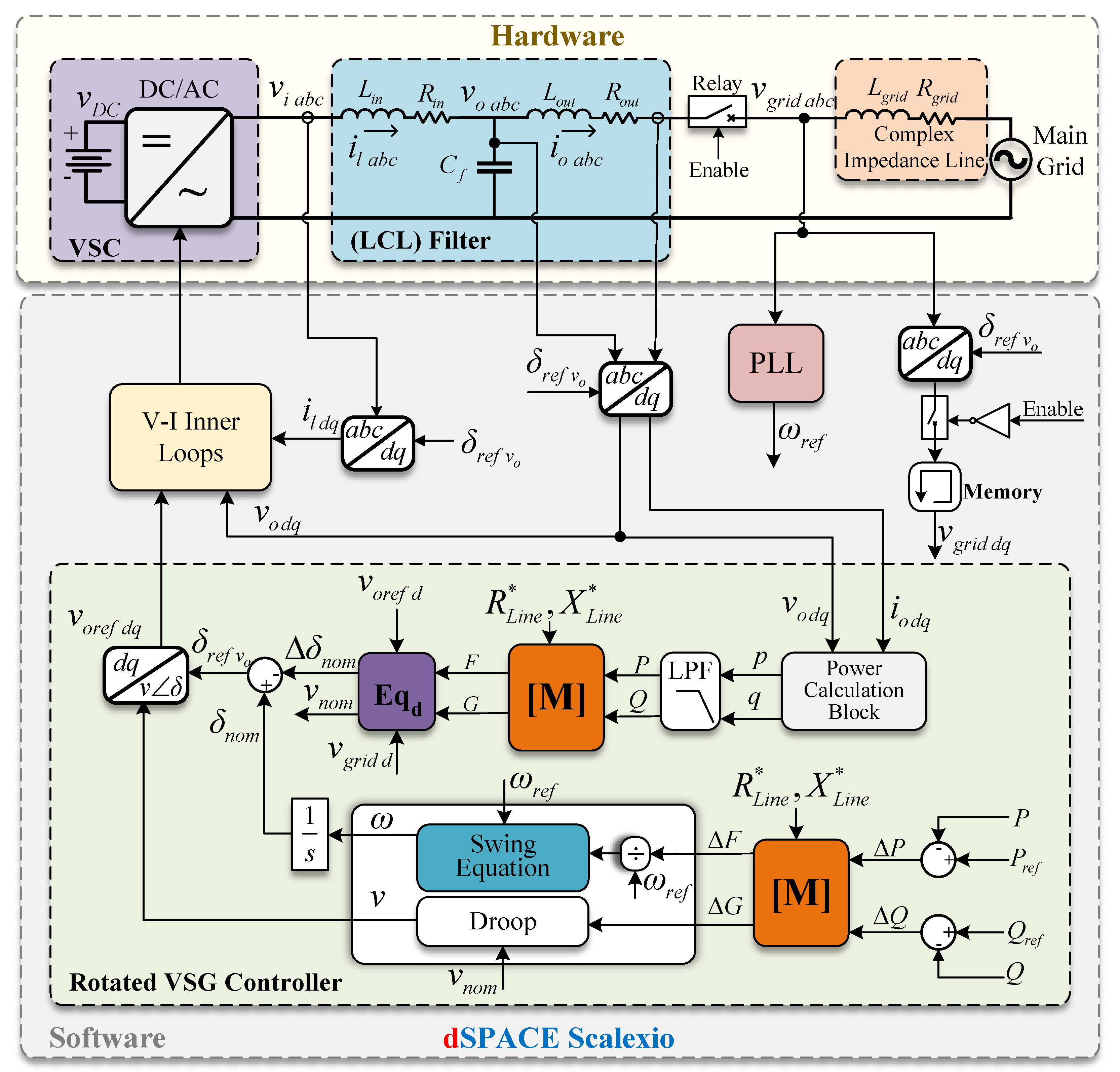
3. Integration of Rotation into VSG Control

This section presents a rotated virtual synchronous generator (RVSG) control method, which uses the new rotated reference frame approach described in the previous section. The RVSG control method allows the emulation of the same behavior of the virtual inertia in a VSC, improving the VSG method presented by Driesen and Visscher [17]. This control scheme is similar to the VSG method, which is located in the active power control loop [18]. The proposed control approach allows for fulfilling the premise of decoupling active and reactive power, achieving better performance. Figure 2 depicts how the RVSG is implemented.

The new rotational reference frame (8) and the behavior of a traditional swing equation, (3) are executed in the proposed RVSG. The rotated power droop control of G, which is responsible for controlling the voltage amplitude (13), is similar to proportional reactive power droop control. As a result, the power control law of the RVSG is as follows:

$$2H\dot{\omega }=\left(\frac{\Delta F}{{\omega }_{ref}}\right)-K_D(\omega -{\omega }_{ref})$$

(11)

$$\omega -{\omega }_{ref}=\left(\frac{1}{2Hs+K_D}\right)\left(\frac{\Delta F}{{\omega }_{ref}}\right)$$

(12)

$$v-v_{nom}=-k_G\Delta G$$

(13)

where $K_D$ is the damping coefficient, H is the virtual inertia constant, $\dot{\omega }$ is the angular acceleration of the RVSG, $\omega$ is the RVSG controller output frequency, which is integrated to obtain the angle ${\delta }_{nom}$, and v is the RVSG controller output voltage. $K_G$ is the slope of the rotated droop controller of G. ${\omega }_{ref}$ and $v_{nom}$ are the frequency and voltage references, respectively.

For practical purposes, the line impedances $R_{Line}^{*}$ and $X_{Line}^{*}$ are used in the transformation matrix of the new frame of reference (8), where $R_{Line}^{*}$ and $X_{Line}^{*}$ contain the sum of the output impedance of the LCL filter and the grid impedance end to the AC bus connection point. Therefore, the line impedance values (R) and (X) equate to $R_{Line}^{*}$ and $X_{Line}^{*}$.

To interface with the voltage and frequency coming from outside the RVSG, the voltage and reference angle required for the inverter operation must be converted to the new reference frame. For this purpose, Equations (14) and (15) are used to solve the nominal voltage $\left(v_{nom}\right)$ and delta angle $(\Delta {\delta }_{nom})$. Using the concept that when the VSC is synchronized, the phase angle between the inverter voltages and the Point of Common Coupling (PCC) must be close to zero, it is assumed that $sin\delta \approx \delta$ and $cos\delta \approx 1$.

These equations are implemented in block $E{q}_d$, as depicted in Figure 2, where (14) and (15) can be expressed as follows:

$$v_{nom}=\frac{v_{gridd}+\sqrt{\left(v_{gridd}^2+4G\right)}}{2}$$

(14)

$$\Delta {\delta }_{nom}=\frac{F}{v_{orefd}{v}_{gridd}}$$

(15)

where $v_{gridd}$ is the grid voltage magnitude, which is measured once at the PCC, before connecting the inverter, and $v_{orefd}$ is the inverter reference output voltage.

4. Model of a Voltage Source Converter with RVSG Control

Following the same approach presented in [19,20], the small-signal state-space model for the RVSG controller was achieved. Considering the external power control loop the output filter, and the impedance grid used as mentioned previously, where the external power control loop setpoints for the amplitude of the voltage and frequency on the inverter output are determined according to the RVSG control law using the Equations (10), (12), and (13), as explained in the previous section. Due to their quick reaction times in comparison to the rest of the system, the inner control loops (voltage and current) are not taken into account in this modeling, so a simplified state-space model is presented. Therefore, having a simplified model offers the advantage of focusing on the behavior of the eigenvalues corresponding to the power dynamics and thus identifying the factors that affect the stability of the system. A linear system with inputs u, outputs y, and state variables x has the following generic structure in the state space:

$$\begin{array}{c}\dot{x}\left(t\right)=Ax\left(t\right)+Bu\left(t\right)\\ y\left(t\right)=Cx\left(t\right)+Du\left(t\right)\end{array}$$

(16)

where A is the state matrix, B is the input matrix, C the output matrix, and D the direct transmission matrix.

By taking into account a complex line impedance, the small-signal state-space power controller model for the RVSG may be described as follows:

$$\left[\begin{array}{c}\dot{\Delta \omega }\\ \Delta F\\ \Delta G\end{array}\right]=A_c\left[\begin{array}{c}\Delta \omega \\ \Delta F\\ \Delta G\end{array}\right]+B_c\left[\begin{array}{c}\Delta i_{ldq}\\ \Delta v_{odq}\\ \Delta i_{odq}\\ \Delta {\omega }_{com}\\ F^{*}\\ G^{*}\\ V_d^{*}\\ V_q^{*}\end{array}\right]$$

(17)

$$\left[\begin{array}{c}\Delta \omega \\ \Delta V_{od}\\ \Delta V_{oq}\end{array}\right]=\left[\begin{array}{c}{C}_{c\omega }\\ C_{cV}\end{array}\right]\left[\begin{array}{c}\Delta \omega \\ \Delta F\\ \Delta G\end{array}\right]+D_c\left[\begin{array}{c}\Delta i_{ldq}\\ \Delta v_{odq}\\ \Delta i_{odq}\\ \Delta {\omega }_{com}\\ F^{*}\\ G^{*}\\ V_d^{*}\\ V_q^{*}\end{array}\right]$$

(18)

where the matrices in (17) and (18) are explained in (19). $B_c$, $C_c$, and $D_c$ are made up of several sub-matrices, which can be found by means of Equations (12) and (13).

$$\begin{array}{c}{A}_c=\left[\begin{array}{ccc}-\frac{K_D}{2H}& -\frac{1}{2H{\omega }_{ref}}& 0\\ 0& -{\omega }_{filter}& 0\\ 0& 0& -{\omega }_{filter}\end{array}\right]\\ \\ B_c=\left[\begin{array}{cccc}{B}_{c_T}& B_{c_{{\omega }_{com}}}& B_{c_{FG}}& B_{c_{V^{*}}}\end{array}\right]\\ \begin{array}{c}\\ C_{c\omega }=\left[\begin{array}{ccc}1& 0& 0\end{array}\right]& C_{cV}=\left[\begin{array}{ccc}0& 0& -k_G\\ 0& 0& 0\end{array}\right]\end{array}\\ \\ D_c=\left[\begin{array}{cccc}{D}_{c_T}& D_{c_{{\omega }_{com}}}& D_{c_{FG}}& D_{c_{V^{*}}}\end{array}\right].\end{array}$$

(19)

where

$$\begin{gathered} \begin{array}{c}{B}_{c_T}={\omega }_{filter}\left[\begin{array}{cccccc}0& 0& 0& 0& 0& 0\\ 0& 0& {\tilde{a}}_v& {\tilde{b}}_v& {\tilde{a}}_i& {\tilde{b}}_i\\ 0& 0& {\tilde{c}}_v& {\tilde{a}}_v& {\tilde{b}}_i& {\tilde{c}}_i\end{array}\right]\end{array} \\ \begin{array}{cc}{B}_{c_{{\omega }_{com}}}=\left[\begin{array}{c}-1\\ 0\\ 0\end{array}\right]& B_{c_{V^{*}}}=\left[zeros(3,2)\right]\end{array}{B}_{c_{FG}}=\left[\begin{array}{cc}\frac{1}{2H{\omega }_{ref}}& 0\\ 0& 0\\ 0& 0\end{array}\right]. \end{gathered}$$

(20)

$$\begin{gathered} \begin{array}{cc}{D}_{c_T}=\left[zeros(3,6)\right]& D_{c_{{\omega }_{com}}}=\left[zeros(3,1)\right]\end{array} \\ \begin{array}{cc}{D}_{c_{FG}}=\left[\begin{array}{cc}0& 0\\ 0& k_G\\ 0& 0\end{array}\right]& D_{c_{V^{*}}}=\left[\begin{array}{cc}0& 0\\ 1& 0\\ 0& 1\end{array}\right].\end{array} \end{gathered}$$

(21)

${\tilde{a}}_v=X{i}_{od}+R{i}_{oq}$, ${\tilde{b}}_v=X{i}_{oq}-R{i}_{od}$, ${\tilde{c}}_v=R{i}_{od}-X{i}_{oq}$, ${\tilde{a}}_i=X{v}_{od}-R{v}_{oq}$, ${\tilde{b}}_i=X{v}_{oq}+R{v}_{od}$, ${\tilde{c}}_i=R{v}_{oq}-X{v}_{od}$

It is crucial to emphasize that this approach’s state-space model is based on a grid-connected system, unlike [19,20]. The component matrix $B_{c_T}$ from matrix $B_c$, which incorporates the rotation reference frame into the state-space model, is another distinction. The $\Delta$ values from the $u\left(t\right)$ input matrix are shown in (18).

The linearized state-space model may be described as follows using the same approach as the control power and the linearized small-signal model of the output (LCL) filter [19].

$$\left[\begin{array}{c}\dot{\Delta i_{Ldq}}\\ \Delta v_{odq}\\ \Delta i_{odq}\end{array}\right]=A_{\left(LCL\right)}\left[\begin{array}{c}\Delta i_{Ldq}\\ \Delta v_{odq}\\ \Delta i_{odq}\end{array}\right]+B_{\left(LCL\right)}\left[\begin{array}{c}\Delta \omega \\ \Delta v_{idq}\\ \Delta v_{griddq}\end{array}\right]$$

(22)

$$\left[\begin{array}{c}\Delta i_{Ldq}\\ \Delta v_{odq}\\ \Delta i_{odq}\end{array}\right]=C_{\left(LCL\right)}\left[\begin{array}{c}\Delta i_{ldq}\\ \Delta v_{odq}\\ \Delta i_{odq}\end{array}\right]+D_{\left(LCL\right)}\left[\begin{array}{c}\Delta \omega \\ \Delta v_{idq}\\ \Delta v_{griddq}\end{array}\right]$$

(23)

where $A_{\left(LCL\right)}$, $B_{\left(LCL\right)}$, and $C_{\left(LCL\right)}$ are the state, input, and output matrices of the state-space model of the output LC filter and the coupling line impedance, respectively. It is important to mention that matrix $C_{\left(LCL\right)}$ is an identity matrix of length six used to see the state values, and $D_{\left(LCL\right)}$ is equal to the zero matrices. The matrices of (22) are defined in (24). It can be seen that matrix $B_{\left(LCL\right)}$ is composed of different sub-matrices, which are defined in (25).

$$\begin{array}{c}{A}_{\left(LCL\right)}=\left[\begin{array}{cccccc}-\frac{R_{in}}{L_{in}}& \omega & -\frac{1}{L_{in}}& 0& 0& 0\\ -\omega & -\frac{R_{in}}{L_{in}}& 0& -\frac{1}{L_{in}}& 0& 0\\ \frac{1}{C_f}& 0& 0& \omega & -\frac{1}{C_f}& 0\\ 0& \frac{1}{C_f}& -\omega & 0& 0& -\frac{1}{C_f}\\ 0& 0& \frac{1}{L_{Line}}& 0& -\frac{R_{Line}}{L_{Line}}& \omega \\ 0& 0& 0& \frac{1}{L_{Line}}& -\omega & -\frac{R_{Line}}{L_{Line}}\end{array}\right]\\ \\ B_{\left(LCL\right)}=\left[\begin{array}{ccc}{B}_{{\left(LCL\right)}_1}& B_{{\left(LCL\right)}_2}& B_{{\left(LCL\right)}_3}\end{array}\right]\end{array}$$

(24)

where

$$\begin{array}{c}{B}_{{\left(LCL\right)}_1}={\left[\begin{array}{cccccc}{i}_{lq}& -i_{ld}& v_{oq}& -v_{od}& i_{oq}& -i_{od}\end{array}\right]}^T\\ \\ B_{{\left(LCL\right)}_2}={\left[\begin{array}{cccccc}\frac{1}{L_{in}}& 0& 0& 0& 0& 0\\ 0& \frac{1}{L_{in}}& 0& 0& 0& 0\end{array}\right]}^T\\ \\ B_{{\left(LCL\right)}_3}={\left[\begin{array}{cccccc}0& 0& 0& -\frac{1}{L_{Line}}& 0& 0\\ 0& 0& 0& 0& 0& -\frac{1}{L_{Line}}\end{array}\right]}^T\end{array}$$

(25)

The whole model of an inverter may be generated by combining the output LC filter, coupling grid impedance, and the small-signal state-space model of the power controller. By combining all the state-space models presented in (17), (18), (22), and (23), it can be described as follows:

$$\begin{gathered} \begin{array}{c}\left[\begin{array}{c}\Delta {\dot{x}}_T\end{array}\right]=A_T\left[\begin{array}{c}\Delta x_T\end{array}\right]+B_T\left[\begin{array}{c}{u}_T\end{array}\right]\end{array} \\ \left[\begin{array}{c}{y}_T\end{array}\right]=C_T\left[\begin{array}{c}\Delta x_T\end{array}\right]+D_T\left[\begin{array}{c}{u}_T\end{array}\right] \end{gathered}$$

(26)

where $\Delta x_T$ and $u_T$ are the state and input variables, and $A_T$ and $B_T$ are the state and input matrices of the state-space of the model of the inverter. The output of the model variables is given by $y_T$, where $C_T$ is the identity matrix and $D_T$ is a zero matrix. As a result, a whole inverter’s state variables and related matrices are shown as:

$$\begin{array}{c}\Delta x_T={\left[\begin{array}{cccccc}\Delta \delta & \Delta F& \Delta G& \Delta i_{ldq}& \Delta v_{odq}& \Delta i_{odq}\end{array}\right]}_{9x1}^T\\ \\ A_T={\left[\begin{array}{cc}{\left[\begin{array}{c}{A}_c\end{array}\right]}_{3x3}& {\left[\begin{array}{c}{B}_c\end{array}\right]}_{3x6}\\ \\ {\left[\begin{array}{c}{B}_{\left(LCL\right)12}{C}_{c_{\omega vi}}\end{array}\right]}_{6x3}& {\left[\begin{array}{c}{A}_{\left(LCL\right)}\end{array}\right]}_{6x6}\end{array}\right]}_{9x9}\\ \end{array}$$

(27)

$$\begin{array}{c}{B}_{\left(LCL\right)12}{C}_{c_{\omega v}}={\left[\begin{array}{c}{B}_{{\left(LCL\right)}_1}{C}_{c\omega }\end{array}\right]}_{6x3}+{\left[\begin{array}{c}{B}_{{\left(LCL\right)}_2}{C}_{cV}\end{array}\right]}_{6x3}\\ \\ B_T={\left[\begin{array}{cc}{\left[\begin{array}{c}{B}_{c_{{\omega }_{com}}}\end{array}\right]}_{3x1}& {\left[\begin{array}{c}zeros(3,6)\end{array}\right]}_{3x6}\\ \\ {\left[\begin{array}{c}{B}_{\left(LCL\right)12}\end{array}\right]}_{6x3}{\left[\begin{array}{c}{D}_{C1}\end{array}\right]}_{3x5}& {\left[\begin{array}{c}{B}_{\left(LCL\right)3}\end{array}\right]}_{6x2}\end{array}\right]}_{9x7}\\ \\ B_{\left(LCL\right)12}=\left[\begin{array}{cc}{B}_{\left(LCL\right)1}& B_{\left(LCL\right)2}\end{array}\right]\\ \\ D_{C1}=\left[\begin{array}{ccc}{D}_{c_{{\omega }_{com}}}& D_{c_{FG}}& D_{c_{V^{*}}}\end{array}\right]\\ \\ u_T={\left[\begin{array}{ccccccc}\Delta {\omega }_{com}& F& G& v_{orefd}& v_{orefq}& v_{gridd}& v_{gridq}\end{array}\right]}_{7x1}^T\\ \end{array}$$

5. Small-Signal Stability

In this part, the eigenvalue concept is used to examine the stability of the VSG controllers and the proposed RVSG controller. By changing the line impedance and VSG settings, the eigenvalue behavior of the two controllers is compared. To make the comparison fair, the inner loop parameters, initial conditions, and filter settings are fixed and the same for both scenarios. Each case’s state matrix A is used to determine the system’s eigenvalues using a MATLAB program. In the RVSG case, the matrix used is $A_T$ given by Equation (27). In the VSG case, the matrix used is $A_T$ without internally implementing the proposed rotation. The parameters utilized to conduct the analysis are provided in

Table 1. Setup model parameters RVSG and VSG.

Parameter	Symbol	Value
Fundamental frequency	$\omega$	376.99 rad/s
Inductance of the grid	$L_{grid}$	0.0001 H to 0.002 H
Resistance of the grid	$R_{grid}$	0.2 $\Omega$ to 2.2 $\Omega$
Virtual inertia constant VSG	H	1.42 s
Damping coefficient VSG	$k_D$	14.53 Ns/m
Amplitude droop	$k_G$	0.02 to 0.04 V/VAR
Cut-off frequency of measuring filter	${\omega }_{filter}$	18.85 rad/s
Grid voltage (main AC)	(V)	120 $V_{RMS}$
Inverter output voltage	($V_{od}$)	120.63 $V_{RMS}$
Filter capacitance	$C_f$	8.8 $\mathsf{\mu }$F
Filter inductance	$L_{in},L_{out}$	1.8 mH
Series resistance of the filter inductor	$R_{in},R_{out}$	0.18 $\Omega$

. The modeling uses the grid impedance values and VSG controller parameters shown in Table 1, while the inverter hardware parameters are shown in

Table 2. Inverter parameter values.

Parameter	Symbol	Value
Inductance filter	$L_{in},L_{out}$	0.0018 H
Resistance filter	$R_{in}$, $R_{out}$	0.2 $\Omega$
DC bus voltage	$DC$	400 V
Voltage loop	$k_{pV}$, $k_{rV}$	0.35, 400
Current loop	$k_{pi}$, $k_{ri}$	0.7, 100
Switching frequency	$f_s$	10 $\mathrm{kHz}$

.

5.1. Analysis of the Behavior of the Eigenvalues When Changing the Line Impedance Parameters

Figure 3 illustrates how the eigenvalues for the RVSG and VSG systems respond to variations in the inductance of the line parameter for a case where $R_{Line}^{*}=R_{grid}=0.2$$\Omega$, $H=1.42$ s, $k_D=14.53$ Ns/m, and $k_G=0.028$. In the figure, it can be observed that the increase in the line inductance value $L_{Line}^{*}$ = ($L_{grid}+L_{out}$) makes the system unstable by moving the dominant eigenvalues of the VSG to the right side of the origin. These correspond to the ${\mathit{1}}_C$ cluster represented in the close-up plot made at the poles near the origin. Conversely, it is noted that in the RVSG situation of the ${\mathit{1}}_R$ cluster, the same dominating eigenvalues also move to the right side, but in this instance, the poles stay on the left side of the origin and the system continues to be stable.

In the VSG model, the cluster of real eigenvalues ${\mathit{2}}_C$ shifts to the left side as the line inductance increases, causing those poles to have less influence on the system. Compared to the case of the RVSG, the same eigenvalues corresponding to cluster ${\mathit{2}}_R$ also shift to the left side, but these start closer to the origin, causing those poles to have more influence on the system. Therefore, the transient responses with the ${\mathit{2}}_R$ cluster have small amplitudes and pass away quickly.

In order to see how the eigenvalues behaved when the line resistance parameter was the only one changed, a new study was conducted using the same methodology as the prior analysis. This study shows that the displacement of the entire locus diagram (Figure 3) to the left is caused by an increase in the line resistance value. As a result, every system eigenvalue is moved into a new location that offers quicker dynamics. As the ${\mathit{1}}_R$ and ${\mathit{2}}_R$ clusters are dominant and enhance the stability of the system when rotation is taken into account, this effect provides greater advantages for the RVSG system than for the VSG system.

5.2. Analysis of the Behavior of the Eigenvalues When Changing the VSG Parameters

In this instance, Figure 4 illustrates how the eigenvalues respond to variations in the reactive power coefficient $kG$ for the case where $R_{Line}^{*}=R_{grid}=0.2$$\Omega$, $L_{Line}^{*}=0.0018$ H, $k_D=14.53$ Ns/m, and $H=1.42$ s. Changes in the damping coefficient $K_D$ and in the virtual inertia constant H have minimal impact on the system’s stability and cause the poles to shift relatively little. Variations in these parameters are thus not taken into account. Additionally, it can be seen in Figure 4 that the system becomes unstable for high values of $k_G$ because the eigenvalues of the ${\mathit{1}}_C$ cluster from the VSG move to the right side of the origin. Conversely, in the RVSG scenario, the cluster ${\mathit{1}}_R$ eigenvalues greatly enhance the system performance in comparison to the VSG, keeping the system stable in the face of high values of $k_G$. This indicates that the RVSG permits dealing with quick reactive power responses, in contrast to the VSG. Moreover, the ${\mathit{2}}_R$ and ${\mathit{2}}_C$ eigenvalue clusters behave similarly to the preceding example when the slope of reactive power rises.

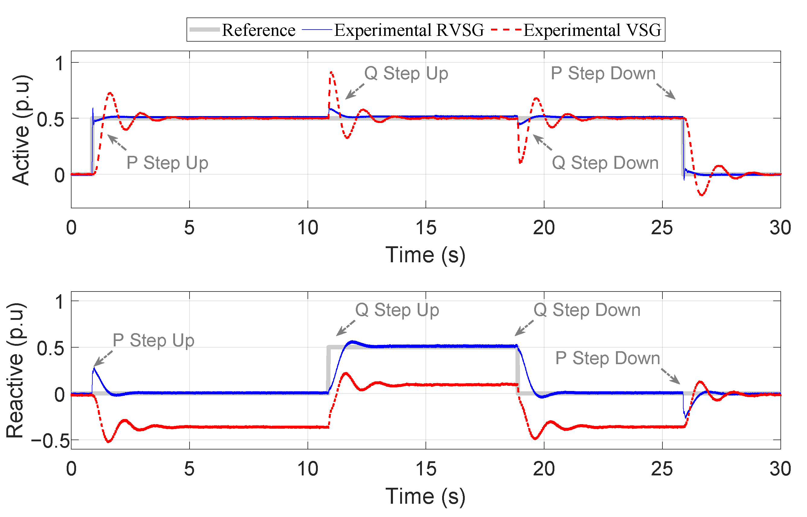
6. Simulation and Experimental Results

As illustrated in Figure 2, a scenario using a VSI is suggested in order to assess the effectiveness of the proposed RVSG controller. The mathematical state-space model that was previously described was used via simulation and was compared behaviorally to the experimental testbed in order to validate the controller. The area marked as Software in Figure 2 corresponds to the RVSG and VSG control algorithms, which were implemented with Matlab Simulink® and compiled using ConfigurationDesk®, downloaded to the dSPACE SCALEXIO platform. The testbed of the microgrid laboratory of the University of Puerto Rico at Matyaguez was used. This testbed contains a Danfoss VLT-302 inverter with LCL filters, a sensor box, and other components. The testbed and the most commonly used control blocks are described in more detail in [18,21,22]. The inverter was synchronized and coupled to the grid at the Point of Common Coupling (PCC) at the beginning of the experiment (before the active power step). The settings in Table 1 and Table 2 were used for both systems to obtain the findings shown in Figure 5 and Figure 6. To monitor the experimental power output, a Low-Pass Filter (LPF) with a bandwidth of 18.85 rad/s was employed.

The active and reactive power responses output from the mathematical model and from the experiment are shown in Figure 5 and Figure 6, respectively, where both RVSG and VSG controllers use the same power step.

The behavior of the experimental system’s output power and the mathematical model using the RVSG controller is shown in the upper part of Figure 5 and Figure 6. The behavior of the output power of the mathematical model and the experimental system using the VSG controller can be seen in the lower part of the same figures (Figure 5 and Figure 6).

Figure 5 and Figure 6 were developed to show that the mathematical model follows the experimental behavior of the power, so the eigenvalues of the previous section agree with the dynamics of the experimental power responses.

Figure 7 shows a comparison between the experimental responses of the active and reactive power for the RVSG and VSG methods; it also shows the changes in the power that are due to power steps and the events that occur due to the power coupling.

The upper part of Figure 7 shows that after 0.5 s, when the active power step occurs, the proposed RVSG reaches the steady state six times faster than the VSG controller, and the overshoot decreases by 30% when comparing the transient responses of the two controllers. Moreover, the active power disturbance in the RVSG controller is 60% less than that in the VSG controller when a reactive power step occurs after 10 seconds. As a result, the RVSG controller’s active and reactive power are less coupled than those of the VSG controller.

The lower part of Figure 7 shows the reactive power response to a 0.5 p.u. step in the reactive power reference, where the steady-state inaccuracy of the reactive power both before and after applying the step in the VSG controller is observed. In contrast, the RVSG controller has a steady-state error of no more than 4%, but the VSG has a steady-state error of more than 20%.

As seen in Figure 4, systems that require quick power responses, particularly for reactive power, are susceptible to entering unstable zones. When VSG controllers are used, the system is slower and performs poorly, which is caused by the utilization of small slope values in the reactive power droop controller. The proposed RVSG control enables the use of greater slope values in reactive power VSG parameters, and thus, a quick reactive power response is expected. Figure 7 shows that the reactive power in the RVSG controller reaches a steady state two times faster than the VSG controller. A summary of the comparison of the dynamic characteristics of the power responses between RVSG and VSG is shown in

Table 3. Comparison of the experimental behavior of the active and reactive power between the RVSG and VSG methods.

	Parameter	VSG	RVSG
Active Power	Settling Time [s]	4.11	0.68
	Rise Time [s]	0.35	0.05
	Overshoot Step Up [%]	45	15
	Steady-State Error [%]	2	2
Reactive Power	Settling Time [s]	3.5	1.8
	Rise Time [s]	0.5	0.4
	Overshoot Step Up [%]	22	10
	Steady-State Error [%]	35	1.2

.

7. Conclusions

This paper presents an RVSG controller that improves the transient response, performance, and precision in power-sharing strategies in microgrids with complex line impedances. It is important to note that the power quality is enhanced by employing a rotational reference frame technique since the coupling of power is reduced.

The rotated reference frame is incorporated into the state-space model provided in this paper.

In order to improve stability under stronger reactive power VSG parameters, this innovative approach enables power-sharing controllers such as the RVSG to be used in microgrids without ignoring the line impedance resistance parameter.

Compared with VSG controllers, the experimental results show that the proposed RVSG has positive effects on the stability and dynamic behavior in power sharing.

A lower steady-state deviation error is observed in the active and reactive power performance of the proposed RVSG for microgrids with complex line impedances.

References

1. Uudrill, J.M. Dynamic Stability Calculations for an Arbitrary Number of Interconnected Synchronous Machines. IEEE Trans. Power Appar. Syst. 1968, PAS-87, 835–844. [Google Scholar] [CrossRef]
2. Beck, H.P.; Hesse, R. Virtual synchronous machine. In Proceedings of the 2007 9th International Conference on Electrical Power Quality and Utilisation, Barcelona, Spain, 9–11 October 2007; pp. 1–6. [Google Scholar] [CrossRef]
3. Chen, Y.; Hesse, R.; Turschner, D.; Beck, H.P. Improving the grid power quality using virtual synchronous machines. In Proceedings of the 2011 International Conference on Power Engineering, Energy and Electrical Drives, Malaga, Spain, 11–13 May 2011; pp. 1–6. [Google Scholar] [CrossRef]
4. Zhong, Q.C.; Weiss, G. Synchronverters: Inverters That Mimic Synchronous Generators. IEEE Trans. Ind. Electron. 2011, 58, 1259–1267. [Google Scholar] [CrossRef]
5. Chen, Y.; Hesse, R.; Turschner, D.; Beck, H.P. Comparison of methods for implementing virtual synchronous machine on inverters. In Proceedings of the International Conference on Renewable Energies and Power Quality (ICREPQ’12), Santiago de Compostela, Spain, 28–30 March 2012; Volume 1. [Google Scholar] [CrossRef]
6. Kundur, P.; Paserba, J.; Ajjarapu, V.; Andersson, G.; Bose, A.; Canizares, C.; Hatziargyriou, N.; Hill, D.; Stankovic, A.; Taylor, C.; et al. Definition and classification of power system stability IEEE/CIGRE joint task force on stability terms and definitions. IEEE Trans. Power Syst. 2004, 19, 1387–1401. [Google Scholar] [CrossRef]
7. Kundur, P. Power System Stability And Control; EPRI Power System Engineering Series; McGraw-Hill: New York, NY, USA, 1994. [Google Scholar]
8. Meng, L.; Savaghebi, M.; Andrade, F.; Vasquez, J.C.; Guerrero, J.M.; Graells, M. Microgrid central controller development and hierarchical control implementation in the intelligent microgrid lab of Aalborg University. In Proceedings of the 2015 IEEE Applied Power Electronics Conference and Exposition (APEC), Charlotte, NC, USA, 15–19 March 2015; pp. 2585–2592. [Google Scholar] [CrossRef]
9. Guerrero, J.M.; Matas, J.; Garcia de Vicuna, L.; Castilla, M.; Miret, J. Decentralized Control for Parallel Operation of Distributed Generation Inverters Using Resistive Output Impedance. IEEE Trans. Ind. Electron. 2007, 54, 994–1004. [Google Scholar] [CrossRef]
10. Li, M.; Shu, S.; Wang, Y.; Yu, P.; Liu, Y.; Zhang, Z.; Hu, W.; Blaabjerg, F. Analysis and Improvement of Large-Disturbance Stability for Grid-Connected VSG Based on Output Impedance Optimization. IEEE Trans. Power Electron. 2022, 37, 9807–9826. [Google Scholar] [CrossRef]
11. Yazdanian, M.; Mehrizi-Sani, A. Distributed Control Techniques in Microgrids. IEEE Trans. Smart Grid 2014, 5, 2901–2909. [Google Scholar] [CrossRef]
12. Saadatmand, S.; Shamsi, P.; Ferdowsi, M. Power and Frequency Regulation of Synchronverters Using a Model Free Neural Network-Based Predictive Controller. IEEE Trans. Ind. Electron. 2021, 68, 3662–3671. [Google Scholar] [CrossRef]
13. Wu, W.; Zhou, L.; Chen, Y.; Luo, A.; Dong, Y.; Zhou, X.; Xu, Q.; Yang, L.; Guerrero, J.M. Sequence-Impedance-Based Stability Comparison Between VSGs and Traditional Grid-Connected Inverters. IEEE Trans. Power Electron. 2019, 34, 46–52. [Google Scholar] [CrossRef]
14. Mohammed, N.; Ravanji, M.H.; Zhou, W.; Bahrani, B. Online Grid Impedance Estimation-Based Adaptive Control of Virtual Synchronous Generators Considering Strong and Weak Grid Conditions. IEEE Trans. Sustain. Energy 2023, 14, 673–687. [Google Scholar] [CrossRef]
15. Park, R.H. Two-reaction theory of synchronous machines generalized method of analysis-part I. Trans. Am. Inst. Electr. Eng. 1929, 48, 716–727. [Google Scholar] [CrossRef]
16. Akagi, H.; Kanazawa, Y.; Nabae, A. Instantaneous Reactive Power Compensators Comprising Switching Devices without Energy Storage Components. IEEE Trans. Ind. Appl. 1984, IA-20, 625–630. [Google Scholar] [CrossRef]
17. Driesen, J.; Visscher, K. Virtual synchronous generators. In Proceedings of the 2008 IEEE Power and Energy Society General Meeting-Conversion and Delivery of Electrical Energy in the 21st Century, Pittsburgh, PA, USA, 20–24 July 2008; pp. 1–3. [Google Scholar] [CrossRef]
18. Campo-Ossa, D.D.; Sanabria-Torres, E.A.; Vasquez-Plaza, J.D.; Patarroyo-Montenegro, J.F.; Lopez-Chavarro, A.F.; Rengifo, F.A. Parametric Comparative Analysis between Virtual Synchronous Generator and Droop-based Inertia for Inverter-Based Microgrids. In Proceedings of the IECON 2021—47th Annual Conference of the IEEE Industrial Electronics Society, Toronto, ON, Canada, 13–16 October 2021; pp. 1–6. [Google Scholar] [CrossRef]
19. Pogaku, N.; Prodanovic, M.; Green, T.C. Modeling, analysis and testing of autonomous operation of an inverter-based microgrid. IEEE Trans. Power Electron. 2007, 22, 613–625. [Google Scholar] [CrossRef]
20. Leitner, S.; Yazdanian, M.; Mehrizi-Sani, A.; Muetze, A. Small-Signal Stability Analysis of an Inverter-Based Microgrid With Internal Model-Based Controllers. IEEE Trans. Smart Grid 2018, 9, 5393–5402. [Google Scholar] [CrossRef]
21. Patarroyo-Montenegro, J.F.; Salazar-Duque, J.E.; Alzate-Drada, S.I.; Vasquez-Plaza, J.D.; Andrade, F. An AC Microgrid Testbed for Power Electronics Courses in the University of Puerto Rico at Mayagüez. In Proceedings of the 2018 IEEE ANDESCON, Cali, Colombia, 22–24 August 2018; pp. 1–6. [Google Scholar] [CrossRef]
22. Vasquez-Plaza, J.D.; Lopez-Chavarro, A.F.; Sanabria-Torres, E.A.; Patarroyo-Montenegro, J.F.; Andrade, F. Benchmarking Real-Time Control Platforms Using a Matlab/Simulink Coder with Applications in the Control of DC/AC Switched Power Converters. Energies 2022, 15, 6940. [Google Scholar] [CrossRef]
Figure 1. Rotation of the power triangle on the proposed reference frame (F and G).
Electronics 12 02156 g001
Figure 2. Control block diagram and power circuit for the implementation of an RVSG in a VSC connected to a main AC source.
Electronics 12 02156 g002
Figure 3. RVSG vs. VSG: Trajectory of eigenvalues of the total system when L l i n e varies from 0.0001 H to 0.002 H.
Electronics 12 02156 g003
Figure 4. RVSG vs. VSG controllers: Trajectory of eigenvalues of total system when k G varies from 0.02 to 0.04.
Electronics 12 02156 g004
Figure 5. Experimental versus modeled active power responses of RVSG and VSG systems.
Electronics 12 02156 g005
Figure 6. Experimental versus modeled reactive power responses of RVSG and VSG systems.
Electronics 12 02156 g006
Figure 7. Experimental active and reactive power responses of RVSG and VSG systems.
Electronics 12 02156 g007