Improving Modulation Recognition Using Time Series Data Augmentation via a Spatiotemporal Multi-Channel Framework

Abstract

Automatic modulation recognition technology with deep learning has a broad prospective owing to big data and computing power. However, the accuracy of modulation recognition largely depends on the massive volume of data and the applicability of the model. Here, to eliminate the difficulties of manual feature extraction, a low accuracy, and a small sample dataset, we propose an effective recognition method that combines time series data augmentation with a spatiotemporal multi-channel learning framework. Compared with other advanced network models, the results showed that the method gave a positive index in the order of 93.5% for ten modulation signal types, which was increased by at least 15%. Especially for QAM16 and QAM64 signals, the average recognition accuracy was improved by nearly 50% at SNRs as low as −2 dB, showing a significant recognition performance. The proposed method provides an attractive method for signal modulation recognition in wireless or wired communication fields.

1. Introduction

Automatic modulation recognition (AMR) can recognize the modulation mode of communication signals received from wireless or wired networks, providing a prerequisite for information extraction [1]. AMR methods are mainly likelihood-based (LB) [2,3] and feature-based (FB) [4]. The LB method has unknown prior knowledge, poor robustness, and complex computations, which are difficult to meet real-time requirements. The FB method designs corresponding classifiers such as the support vector machine (SVM), decision tree [5], and k-nearest neighbor (KNN) algorithms to realize the signal recognition by extracting high-order cumulants [6,7] and instantaneous features [8,9]. It does not require much prior knowledge, so it is widely used. In recent years, with the rapid development of deep learning (DL), its application in the field of signal modulation recognition has made great progress. In 2016, O’Shea et al. first publicized the RadioML2016.10b dataset and constructed a modulation recognition network based on a convolutional neural network (CNN) to capture the signal features from in-phase (I) and orthogonal (Q) components, with an overall recognition accuracy of about 60% of the signal [10,11]. In 2018, O’Shea et al. designed a unique residual module based on a residual neural network (ResNet), with a recognition result of nearly 90% in the end [12]. In the same year, Rajendran et al. modified the dataset by extending the original dataset sampled with 128 points to 512 and used a long short-term memory (LSTM) neural network to identify up to 92% of the results [13]. In the literature [14,15], considering the problem of an I/Q phase signal time series, the fusion of a CNN and LSTM has been able to obtain the spatial and temporal features of the signal from training data; the recognition accuracy was around 93%. In 2020, researchers proposed a CNN–LSTM-based dual-stream structure that divided the signal into two parallel inputs, I/Q and A/P, with a recognition accuracy of up to 92% [16]. In the literature [17,18], constellation map rotation, flip, and random erasing algorithms have been cited as data augmentation techniques combined with LSTM, which eventually achieved a recognition accuracy of about 92%, separately. In [19], a hybrid neural network model MCBL was proposed, which combined a CNN, bidirectional long short-term memory network (BLSTM), and attention mechanism, utilizing their respective capabilities to extract the significant features of space and time embedded in the signal samples; the recognition accuracy reached 93%. To overcome the limitations of a small number of training samples, manual feature extraction, and low recognition accuracy, we proposed a recognition method that combined time series data augmentation and a spatiotemporal multi-channel framework. The expected recognition results were achieved by scaling, magnitude warping, and time warping to expand the amount of data, sample diversity, and feature set. By comparing the mixing efficiency of QAM16 and QAM64 as well as the model complexity with the seven methods in the cited references in terms of the overall signal recognition accuracy, the automatic signal modulation recognition performance of the proposed method was verified and the effectiveness and applicability of the method was demonstrated.

2. Data Augmentation in a Spatiotemporal Multi-Channel Framework

The experimental dataset used by all algorithms was the RadioML2016.10b, generated by the GNU Radio channel model. This dataset introduced pulse shaping, modulation, the characterization of the emission parameters, and the same carrying data as the real signal. It also involved several realistic channel defects such as sample rate offset, additive white Gaussian noise, channel frequency offset, and multi-path fading. The RadioML2016.10b dataset parameters are shown in

Table 1. RadioML2016b dataset parameter introduction.

Parameter	Value
Samples per symbol	4
Sampling rate offset standard deviation	0.01 Hz
Maximum sample rate offset	50 Hz
Maximum carrier frequency offset	500 Hz
Carrier frequency offset standard deviation	0.01 Hz
Sample length	128
SNR range	−20 dB–18 dB
Sampling rate	200 kHz
Number of training samples	720,000
Number of test samples Number of validation samples	240,000 240,000

. The total number of dataset samples was 1,200,000, including 10 modulation signal types under 20 signal-to-noise ratios (SNRs) and all the signal samples were balanced. The ten signal types were 8PSK, AM-DSB, GFSK, BPSK, CPFSK, PAM4, QAM64, QAM16, QPSK, and WBFM, which were represented by two signals, I and Q. The SNR range was −20 dB to 18 dB, with an interval of 2 dB. The signal data format was (2 $\times$ 128). A deep learning algorithm was proposed to automatically predict the modulation category of the radio.

DL is currently being effectively applied to the modulation and recognition of wireless signals. However, the training of DL models requires a large amount of data; a lack of training data causes serious overfitting problems in the model and reduces the classification accuracy. To overcome this problem, data augmentation is widely used in various scenarios. However, in the field of wireless communications, there are few studies exploring the influence of different data augmentation methods on signal modulation classifications. Therefore, we provided three data augmentation methods—namely, scaling, magnitude warping, and time warping—which amplified the signal data without changing the data distribution by changing the amplitude and time axis spacing of the signal. We also designed a spatiotemporal multi-channel framework to evaluate the 3 data augmentation methods and achieved a 93% accuracy when the sample was only 360,000. The following describes how these three methods were implemented.

The scaling generated a scalar through the Gaussian distribution; we multiplied a set of signals by this scalar to achieve an increase or decrease in the amplitude and played the effect of the data scaling. In the equation below, $s_i$ denotes the signal data and $r$ is the scalar generated by the Gaussian distribution.

$$\begin{array}{l}{s}_i^{\ast }=s_i\cdot r\\ r~N(\mu =1,\delta )\end{array}$$

(1)

The processing concept of the magnitude warping was to create three smooth curves from four random coordinate points and then interpolate the obtained three curves through the cubic spline interpolation function to obtain a new smooth curve. Finally, we multiplied this smooth curve with each sample point of the time series to obtain a new signal. In the equation below, $s_i$ denotes the signal data and $r(t_T)$ denotes the time point, which was mathematically expressed as follows:

$$\begin{array}{l}{s}_i^{\ast }=s_i\cdot CubiSpline(r)\\ r=\{r(t_1),\dots ,r(t_T)\}\\ r(t_i)~N(\mu =1,\delta )\end{array}$$

(2)

Time warping is a way to transform the time dimension. It can also be realized by using the smooth curve generated by the cubic spline interpolation function or by a randomly positioned fixed window. The augmented time series could be expressed as:

$$s_i^{\ast }=s_{\gamma (1)},\dots ,s_{\gamma (t)},\dots ,s_{\gamma (T)}$$

(3)

where $\gamma (\cdot )$ is the smooth curve generated by the cubic spline interpolation function. The smooth curves formed by knots $u=u_1,\dots ,u_i,\dots ,u_I$ were defined by the cubic spline. The knots $u_i$ were taken from $u_I~N(1,{\sigma }^2)$.

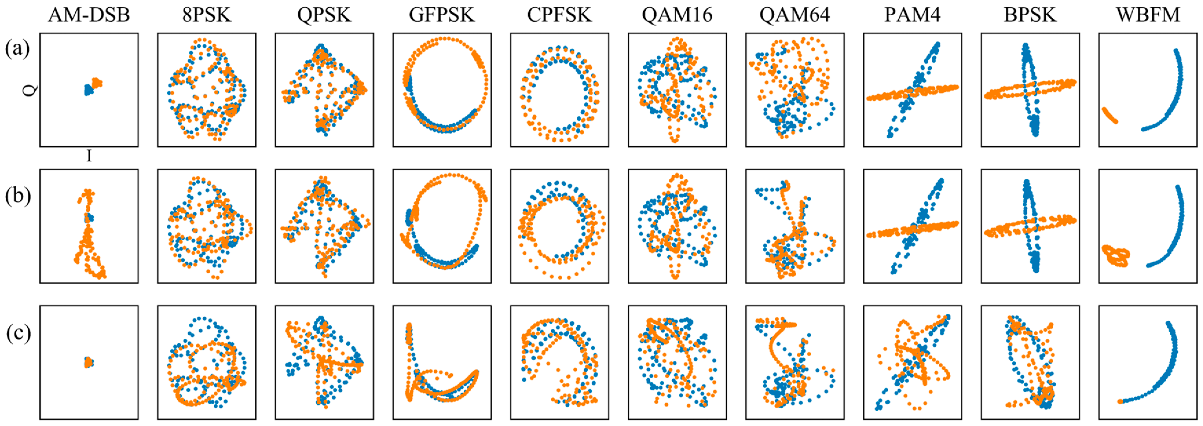
Figure 1 represents a visual comparison plot of the ten modulated signal samples in the dataset after the time series data transformation where the horizontal axis indicates the I-way signal values and the vertical axis indicates the Q-way signal values; this plot represents the signal constellation diagram. Figure 1a–c represent the three data augmentation methods of scaling, magnitude warping, and time warping, respectively. The two methods of scaling and magnitude warping achieved the transformation of the signal amplitude and the method of time warping stretched or compressed the signal on the time axis. 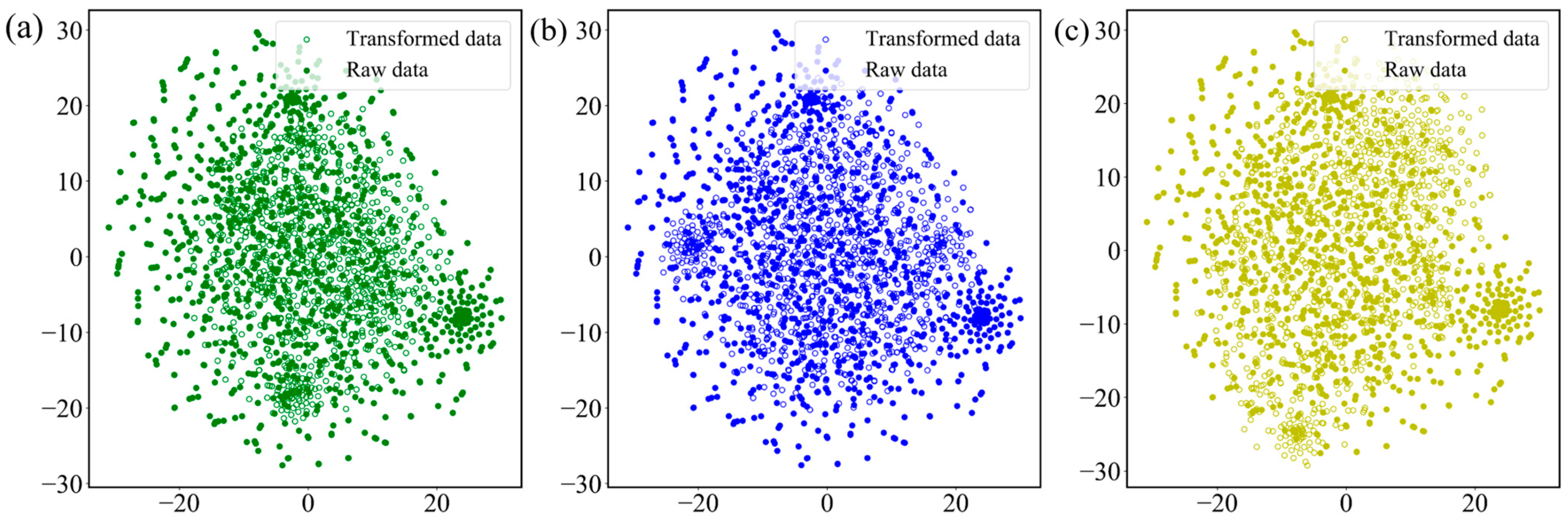Figure 2 shows 3000 samples randomly selected from the overall dataset, which were separately processed by 3 data augmentation methods after the t-SNE visualization algorithm. The t-SNE algorithm played the role of dimensionality reduction, reducing the data of 3000 $\times$ 2 $\times$ 128 to a two-dimensional space for visualization. The solid points in the figure indicate the original dataset distribution and the hollow points illustrate the dataset after the data transformation, which revealed that both performed the role of data augmentation without changing the overall data distribution.

Different from the image signal, the time series data had a temporal correspondence between the samples, so the newly generated samples needed to be considered in this correspondence when enhancing the time series data. Nowadays, there are several types of time series data such as continuous-valued time series, discrete-valued text data, and audio data. Despite the different data types, the applied data augmentation methods (such as adding noise or flipping or stretching) have a common design concept. The three methods proposed in this paper performed dynamic warping and shifting on the amplitude and time axes, respectively, and were able to find combinations of sequences with different amplitudes and time intervals, but with very close morphologies, to achieve the purpose of data augmentation.

In the field of communication systems, AMR can be equivalent to a classification scenario in DL. A CNN extracts the high-dimensional features of signals through convolution, which has advantages in spatial feature extractions. At the same time, LSTM learns the weight of the gate through the input data and the state of the unit and then extracts the time characteristics of the signal, which has advantages in time signal processing. However, if there is an uncertainty (such as different sampling rates), it may be inaccurate to only use a separate model for AMR processing because it only considers the spatial or temporal features and it is difficult to improve the recognition accuracy due to missing feature considerations. Therefore, considering the complementarity of the model, a CNN and LSTM were combined to extract the spatial and temporal characteristics of the signal to achieve the AMR of the signal. 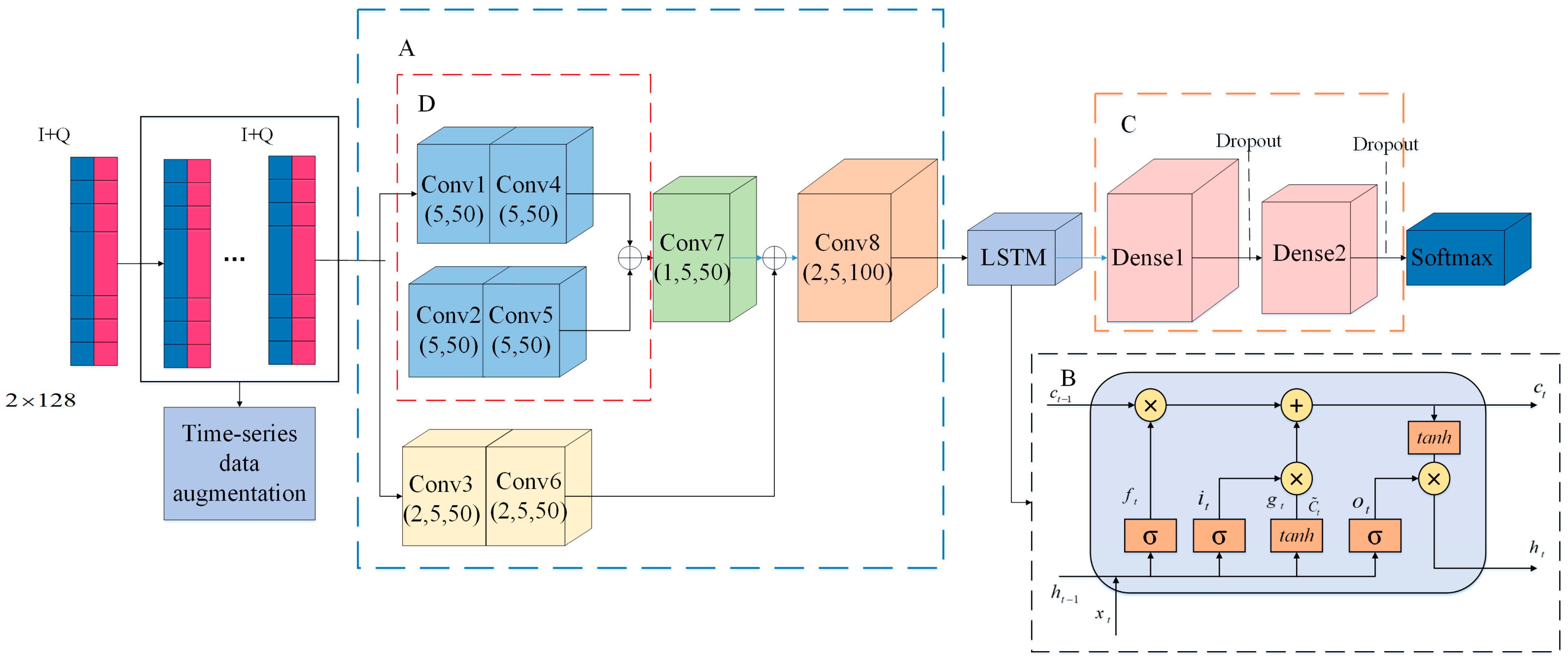Figure 3 shows the frame diagram of the designed network model.

The convolution module consisted of four two-dimensional convolutions (Conv3, Conv6, Conv7, and Conv8) and four one-dimensional convolutions (Conv1, Conv2, Conv4, and Conv5), as shown in Figure 3. The size of each one-dimensional convolution kernel was 5 and the number was 50; the size of the two-dimensional convolution kernel was 1 × 5 and 2 × 5 and the number was 100. The activation function selected was ReLU. First, the I/Q signal was divided into independent I-channel and Q-channel data and then the three sets of data were imported into the convolution module to extract the multi-channel and independent channel features of the I/Q signal. We connected these features and entered Conv7 to determine the spatial correlation. The convolutional module outputted a feature map of 124 × 100 as an input to the LSTM layer, which consisted of 128 memory cells and outputted 128 eigenvectors as an input to the dense layer. To avoid overfitting, both dense layers employed a dropout, whose parameter was set to p = 0.5. The extracted signal features were integrated by the dense layers and finally the classification was completed by the SoftMax function.

3. Results and Discussion

All the following experiments were operated in a python environment using the Google TensorFlow (2.4.1) platform for the computations related to the neural network models. The dataset was first partitioned into the training set, the test set, and the validation set at a ratio of 3:1:1, respectively; the optimizer of Adam was selected, the batch size was set to 128, and the number of iterations was 30. Figure 4 shows that the recognition accuracy of the modulated signals was related to the SNR. With an increase in the SNR, the recognition accuracy also increased. When the SNR was greater than 5 dB, all signals—except WBFM, QAM16, and QAM64—were correctly identified and the recognition accuracy was close to 98%. When the SNR was 0 dB, except for WBFM, the recognition accuracy of the other signals was basically more than 92%. Among them, PAM4 had the best recognition effect and the strongest anti-interference ability against noise. When the SNR was greater than −5 dB, the recognition accuracy reached more than 90%, which was significantly higher than other types of signals. The results showed that the method based on DL could be applied to a modulation recognition task under a low SNR.

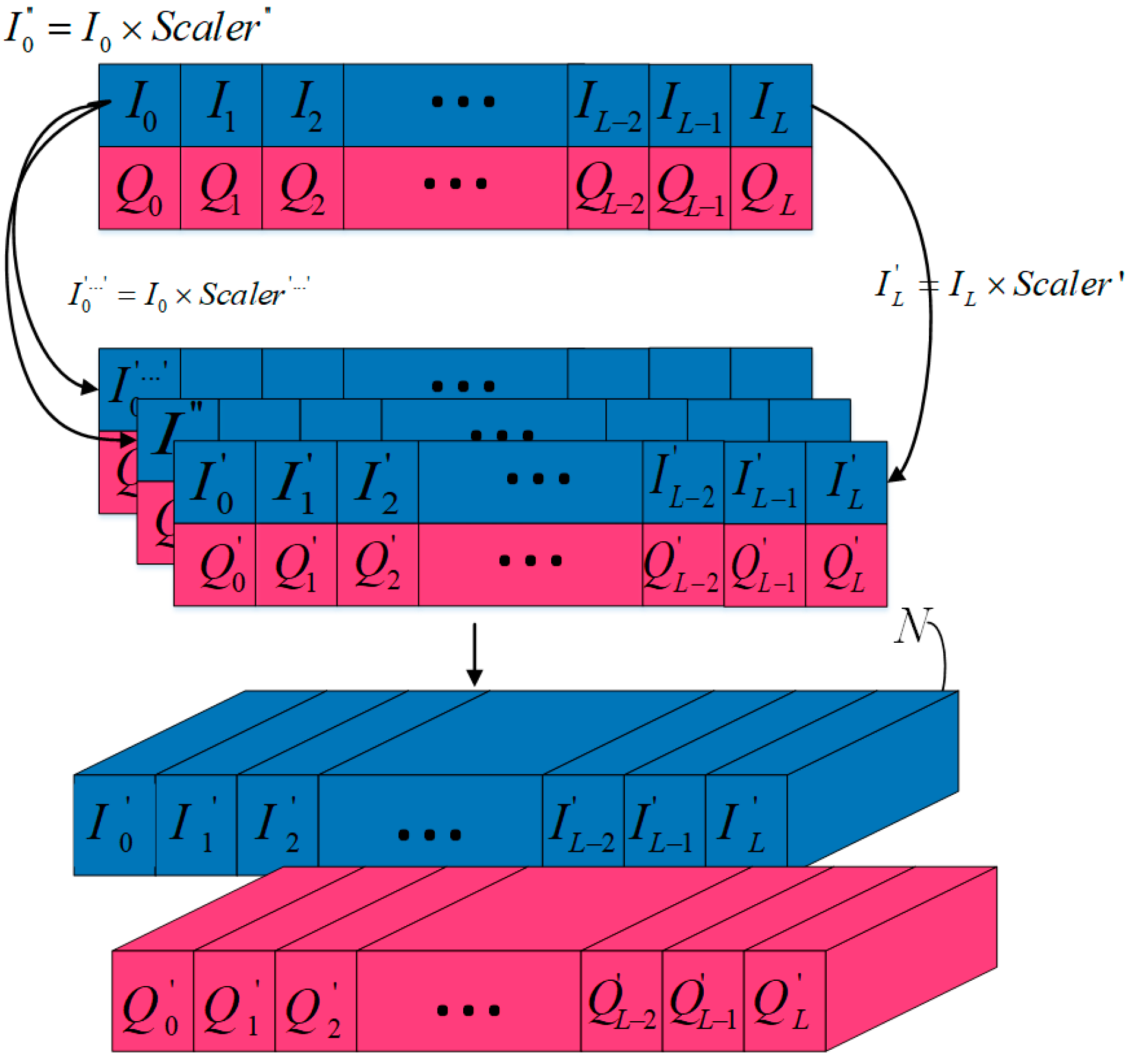
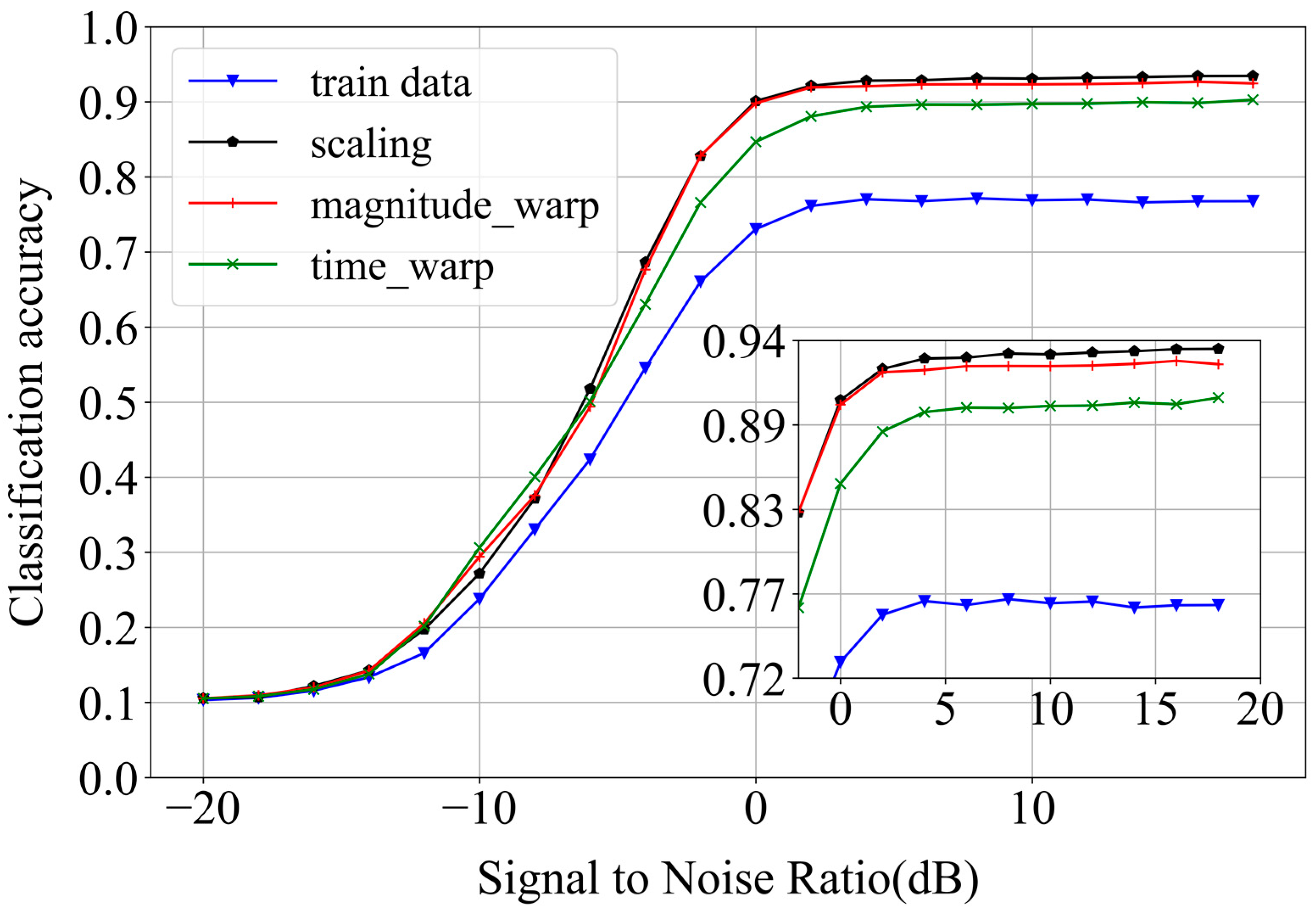
The three data augmentation methods of scaling, magnitude warping, and time warping were extended according to the equal scale factor N = 4. Taking scaling as an example (the transformation process is shown in Figure 5), a scaler was randomly generated by the Gaussian distribution and the original I/Q was multiplied with it to obtain a new set of I/Q signals as new signals. The process was repeated N times to amplify the dataset to N times. A total of 50% of the data in the training set were then randomly sampled as a mini sample training set for the evaluation. The recognition accuracy was about 76%, as shown in the blue curve in Figure 6. The highest recognition accuracies were 93.45%, 92.47%, and 90.27% when the three data augmentation methods of scaling, magnitude warping, and time warping were extended, respectively, according to the equal proportion factor N = 4, resulting in a substantial improvement in the recognition accuracy. Scaling was the most significant; it improved the recognition accuracy by about 17%, showing that all three methods could contribute to data augmentation and were able to enhance the accuracy of the signal recognition under small sample conditions.

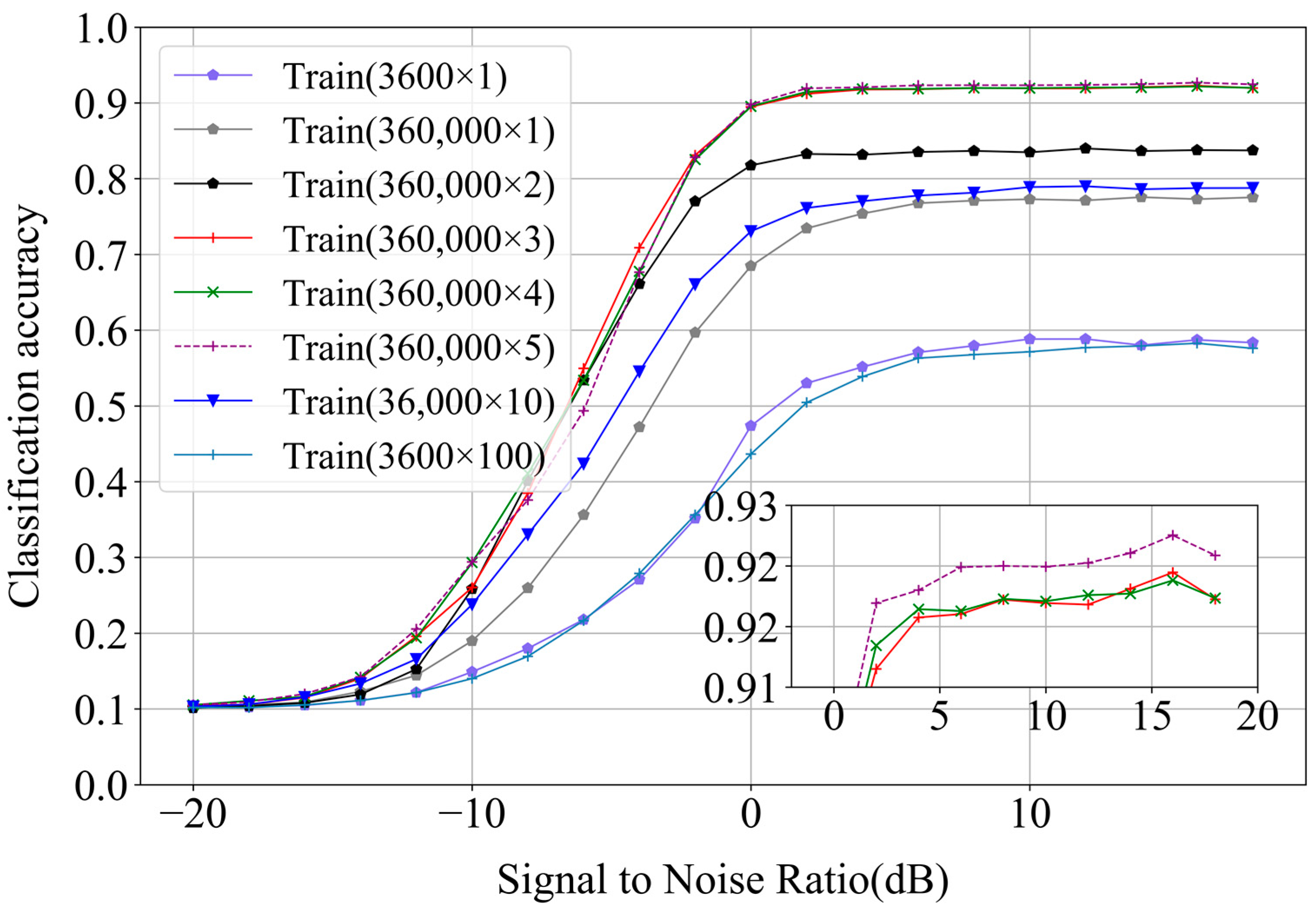
As DL depends on a massive volume of data, the characteristics learned at the front end of the network are entirely derived from existing data. As the amount of data used for learning increases, it is possible for the neural network to learn additional and superior characteristics by obtaining significantly greater amounts of information. Therefore, two sets of experiments were performed to examine the effect of the database size on the network performance by enhancing the dataset with the magnitude warping method as an example. First, 360,000 samples were randomly selected from the original dataset as the training set. The training set samples remained unchanged and different small equal scale factors were used to enhance the training set. In the second group, the original data sizes of 3600 and 36,000 were selected to be enhanced 100 times and 10 times, respectively. The corresponding relationship between the equal scale factor and the data size is shown in

Table 2. Dataset relationship mapping table.

Samples of Raw Data	N	Number of Samples
360,000	1	360,000
360,000	2	720,000
360,000	3	1,080,000
360,000	4	1,440,000
360,000	5	1,800,000
36,000	10	360,000
3600	100	360,000
3600	1	3600

. The results are shown in Figure 7. It could be seen that the total number of samples had a significant impact on the performance of modulation recognition. When the training dataset was only 3600, the training model could not learn more potential features, resulting in less than a 60% accuracy of the signal recognition and poor recognition results. When N was between 1 and 5, the recognition accuracy gradually increased with an increase in the scale factor N. When N = 5, the overall recognition accuracy of the signal reached 93%. However, it could be seen—from the results when the original dataset was expanded 100 times and 10 times—that when the scale factor was too large, the signal recognition accuracy only weakly improved; it was also accompanied by a decrease in the recognition accuracy. We proved, through two sets of experiments, that the method could effectively improve the recognition accuracy of the modulated signals under small sample conditions with a constant scale factor.

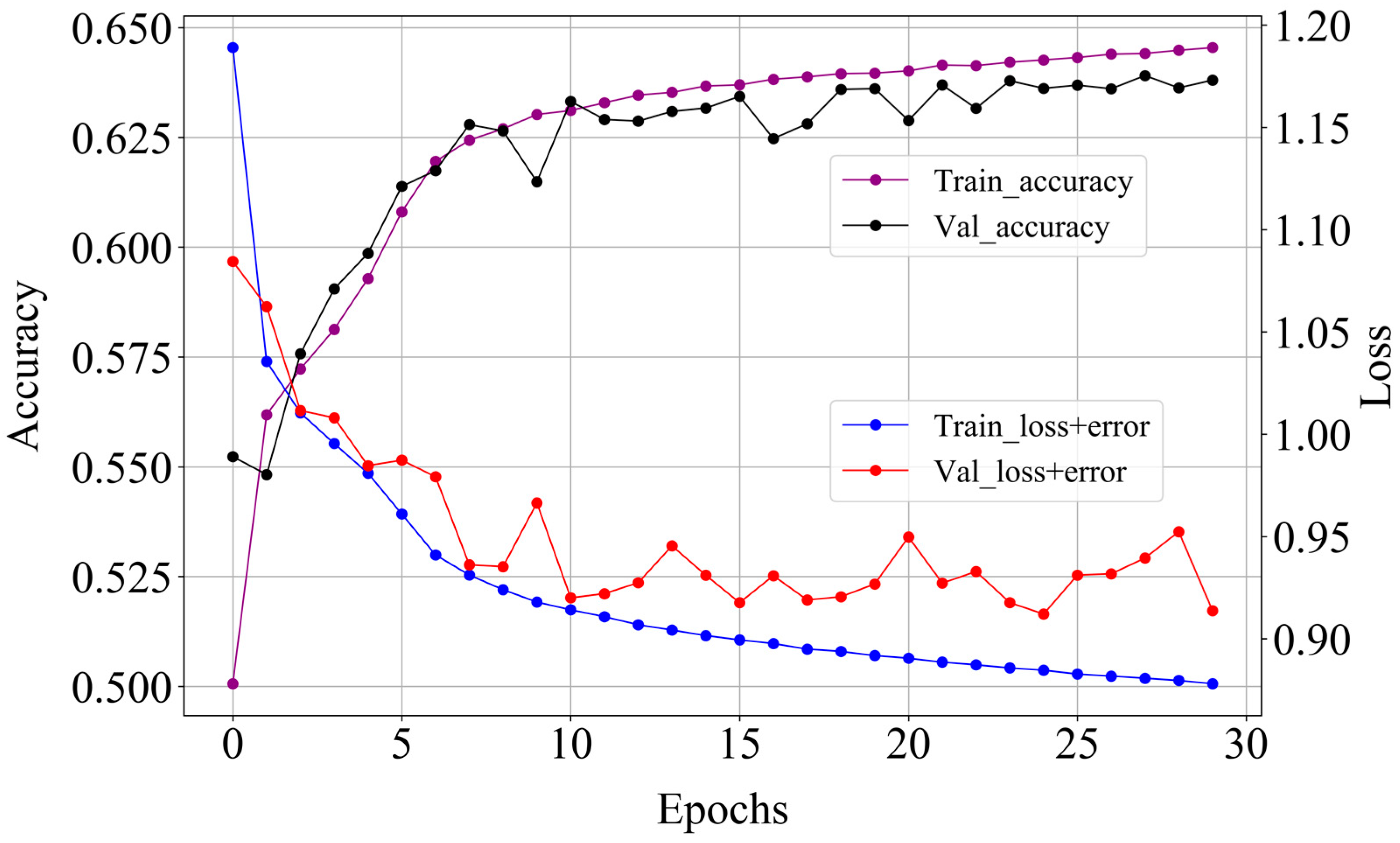
Analyzing from the model perspective, Figure 8 shows the relationship between the loss value and the accuracies with the number of iterations. When the number of iterations increased, the recognition accuracy improved and the loss value of the function gradually decreased, which indicated that the convergence of the model was satisfactory. The loss function curve of the training set was still falling when the training count reached 30, but the validation set had an upward tendency. This indicated that if the model continued to be overfitted by the training, the model had stabilized at this time. It was demonstrated that the network model designed in this paper reasonably generalized that it could be applied to the modulated signal identification problem.

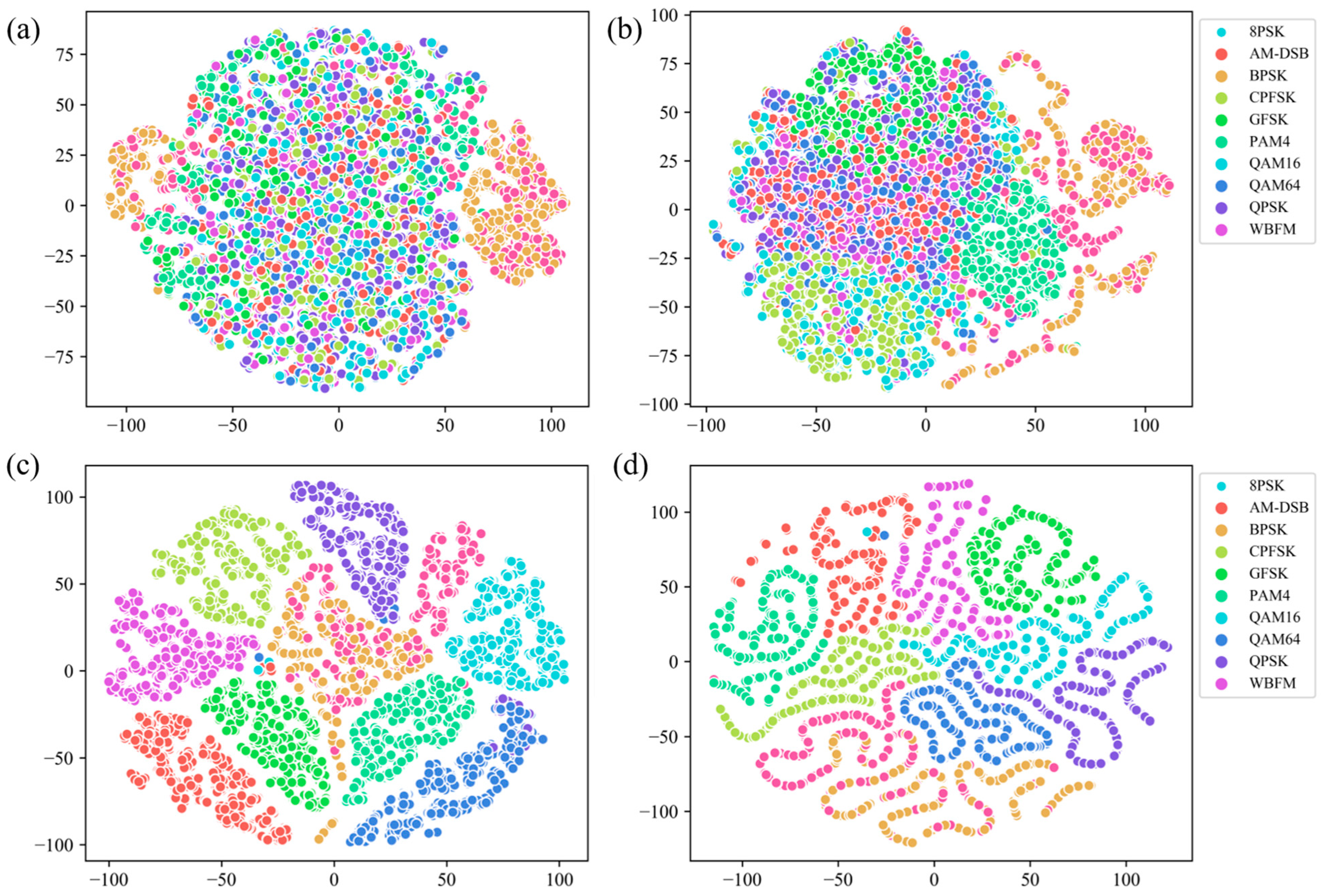
In order to visually understand the effectiveness of the model classification, the characteristics of the output layer of the neural network were converted into a two-dimensional scatter plot, as shown in Figure 9, by the t-SNE visualization algorithm. It is clear from the figure that there was a significant overlap between the signals that had not been modeled and it was impossible to distinguish between each modulated signal. After the CNN processing, this overlapping phenomenon was alleviated to a certain extent; after LSTM processing, the features became obviously separable and the classification effect was greatly improved. Finally, through DNN and SoftMax processing, the signal could basically be separated. Therefore, the proposed network model had a strong discrimination and separability.

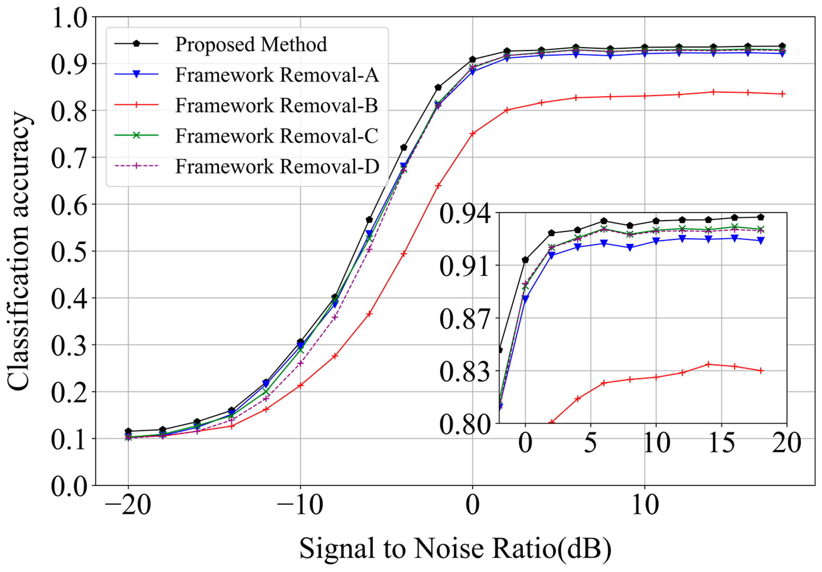
We established four independent modules to discuss the impact of the different modules on the overall structure, which were Framework-A (which removed the independent channel parts from the overall framework), Framework-B (which removed the LSTM), Framework-C (which removed the FC), and Framework-D (which removed the convolution modules). The experimental results showed that the removal of the LSTM module led to a significant decline in the recognition performance (Figure 10), indicating the importance of time modeling for the input data. The combined model recognition results showed that the advantages of each module were complementary; more feature information could be extracted and the accuracy of the signal modulation recognition was effectively improved.

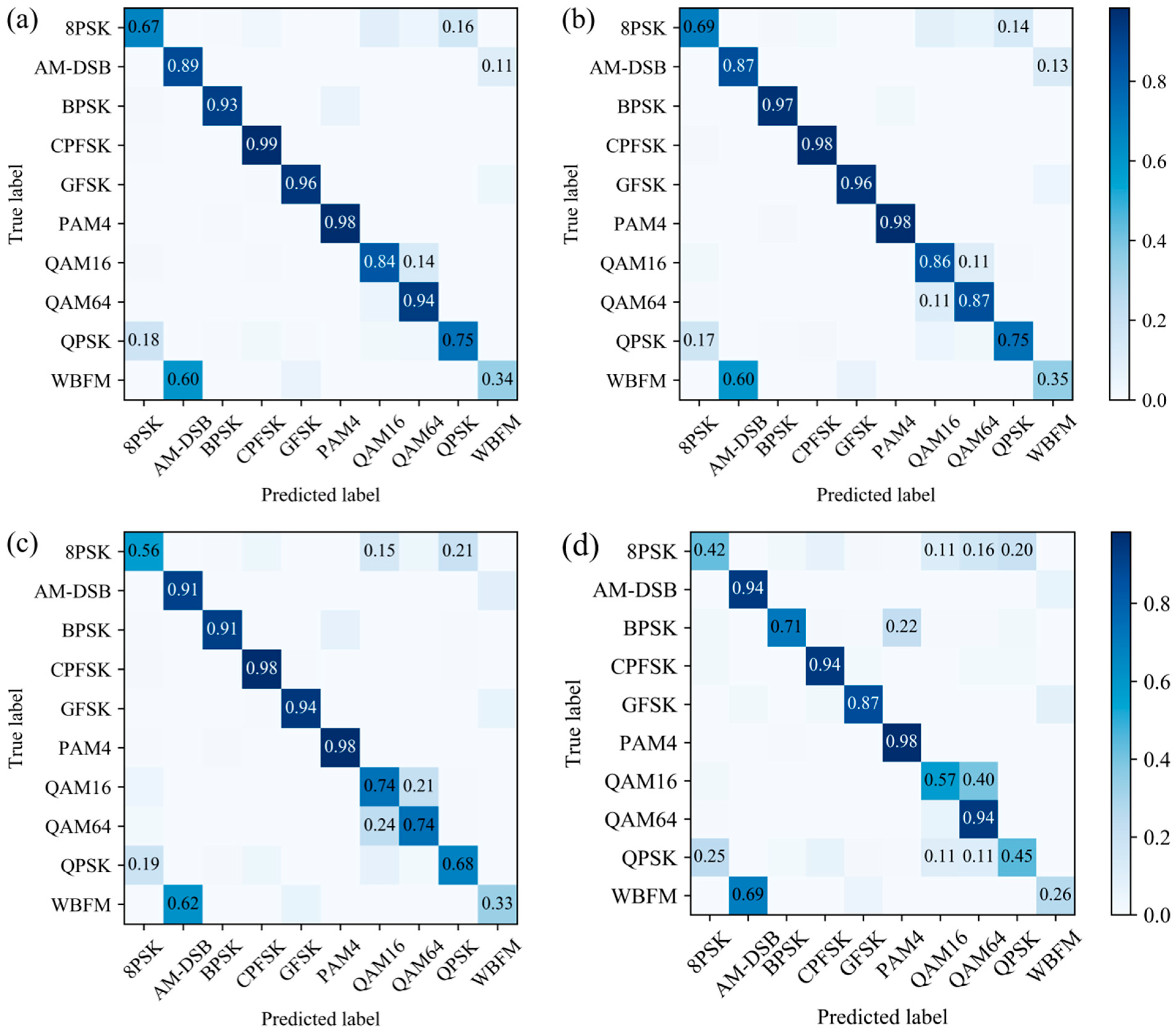
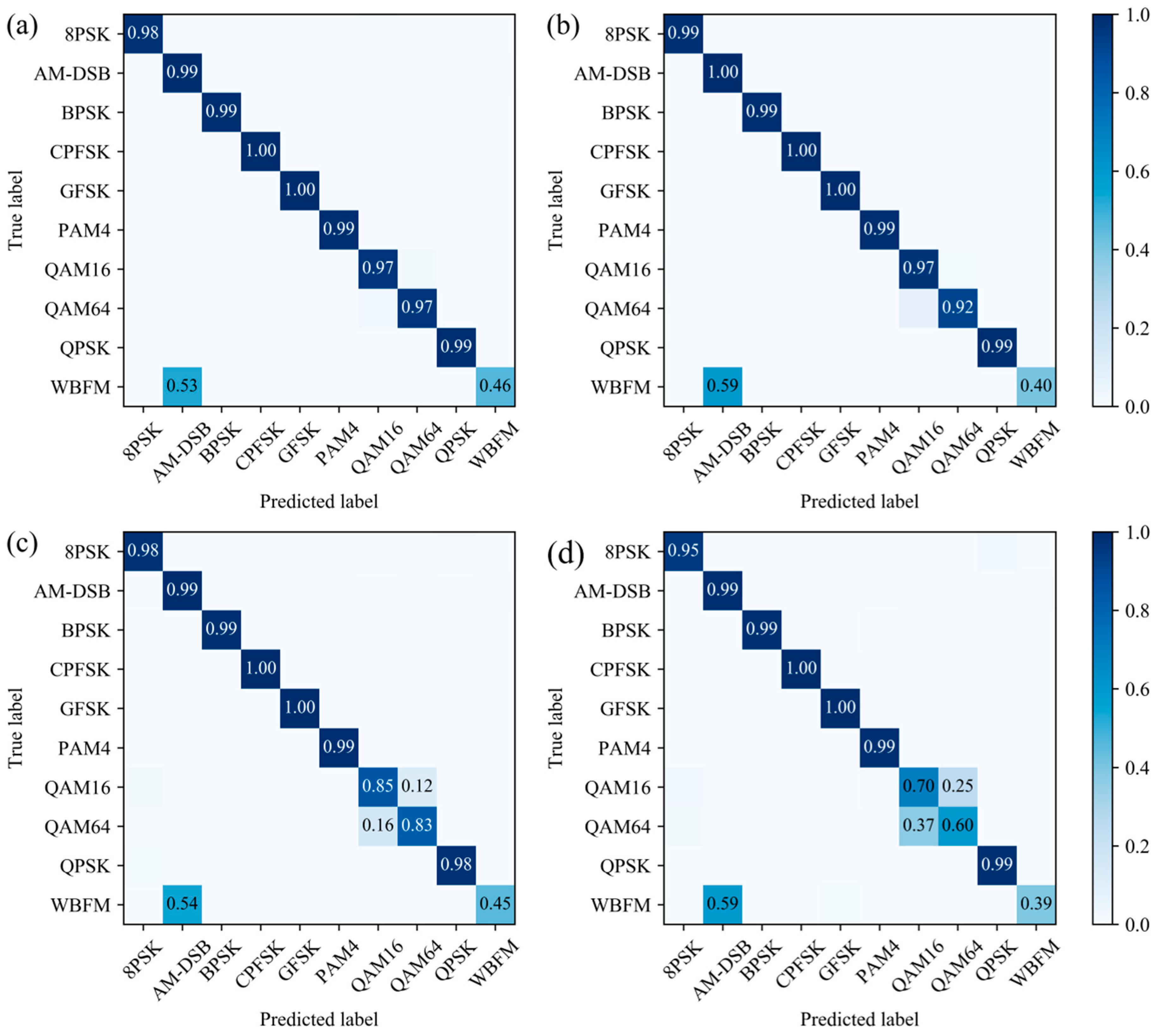
Figure 11 and Figure 12 represent the comparison plots of the confusion matrix obtained from the small sample training set processed by the three data augmentation methods and the original training set after the model at signal-to-noise ratios of −2 dB and 18 dB. The diagonal values in the figure indicate the recognition accuracy of the corresponding signal; the signal recognition accuracy improved as the signal-to-noise ratio increased. Figure 11d shows that the QAM64 and QAM16, as well as the WBFM and AM-DSB, signals were confused for reasons explained in the literature [10,20]. WBFM and AM-DSB both belonged to the continuous modulation and the obvious features between them were very weak in the complex panels. The WBFM and AM-DSB data in the dataset were generated by sampling analog audio signals and the small observation window of both signals (0.64 ms modulated speech per sample) led to a low information rate that was prone to silence between words, making the situation worse and more difficult to identify. When distinguishing between QAM16 and QAM64, only a few symbols could be seen from the short observation time. Moreover, the constellations of the two were of a higher order and had something in common, which made it difficult to distinguish the two signals. It was also the main reason why the overall recognition accuracy reached 93%, with an impossibility of further improvement. However, as seen in the figure, the three methods of scaling, magnitude warping, and time warping all improved the level of confusion between QAM64 and QAM16 to increase the recognition accuracy of both signals, in which scaling had the highest performance. Overall, for all modulation classes, there were three data augmentation methods that could better solve the confusion problem of QAM16 and QAM64 and thus improve the recognition accuracy of the signals.

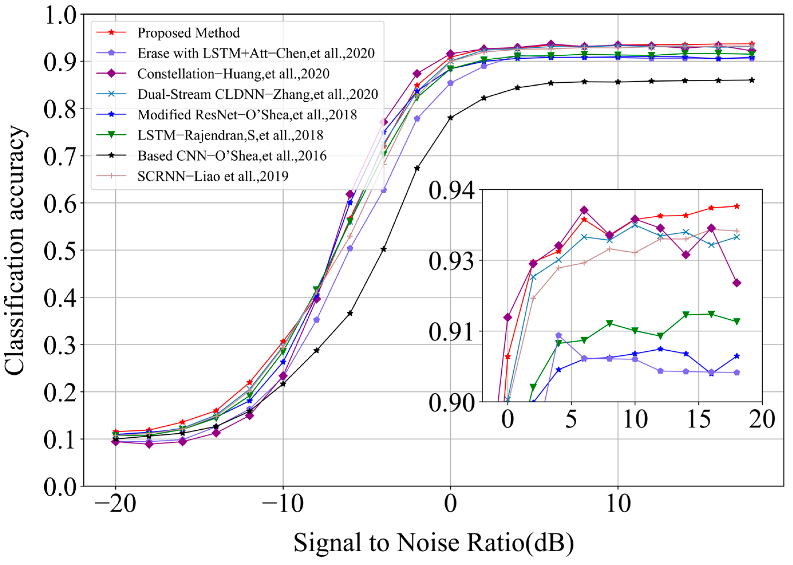
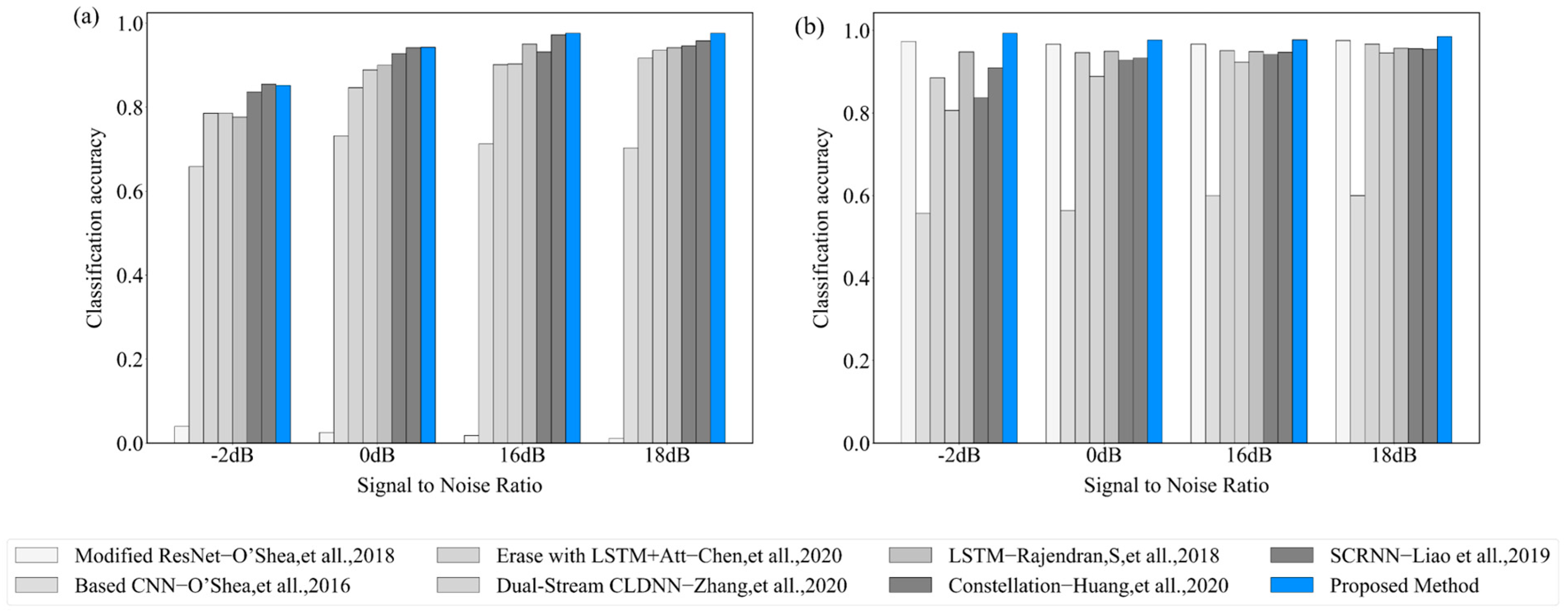
To demonstrate the effectiveness of the combination of data augmentation and the spatiotemporal multi-channel learning framework, we compared the proposed approach with six existing network models [11,12,13,14,16,18]. All of the above classifications were balanced and used the RadioML2016.10 b dataset; the results are shown in Figure 13. In this paper, we combined data augmentation methods with multiple neural network models (CNN, LSTM, and DNN) and designed three channels of parallel input data to achieve the feature fusion. Only half of the samples in the training set were required for training, achieving a maximum recognition accuracy of 93.68%. 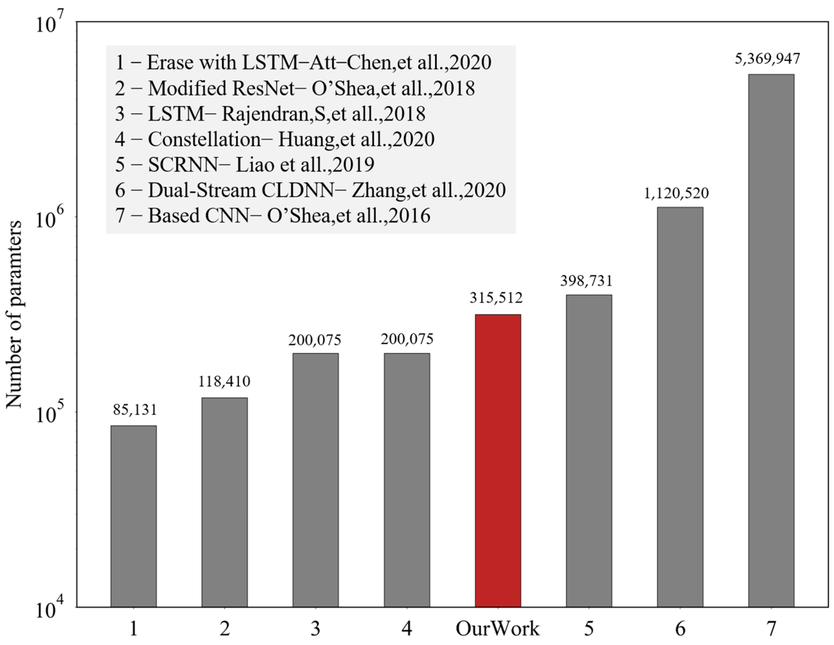Moreover, the confusion problem of QAM16 and QAM64 was eliminated and the recognition accuracy of the two signals was highest, as shown in Figure 14, when comparing the proposed algorithm with the above six algorithms. From the perspective of the computational complexity, as shown in Figure 15, the recognition accuracy of both reference [11], which involved the most parameters, and reference [12], which had the least parameters, failed to achieve rational results. The model designed in this paper involved 315,512 parameters, with relatively few parameters, and was always at a high level in terms of the recognition accuracy. The comprehensive comparison results are shown in

Table 3. Comprehensive comparison of the results of different models.

Model	Accuracy	AccQAM16 (18 dB)	AccQAM64 (18 dB)	Model Complexity
CNN-Based [11]	85.89%	70.29%	59.96%	5,369,947
Modified ResNet [12]	90.99%	1.17%	97.54%	118,410
LSTM [13]	91.63%	94.16%	95.66%	200,075
SCRNN [14]	92.87%	98.79%	95.45%	398,731
Dual-Stream CLDNN [16]	93.33%	93.56%	94.56%	1,120,520
Constellation [17]	93.61%	94.58%	95.58%	200,075
Erase with LSTM + Att [18]	90.58%	91.68%	96.68%	85,131
Our Work	93.68%	97.63%	98.54%	315,512

. Compared with the previous work, our work had a medium model complexity and better results in the overall recognition accuracy and confusion degree of QAM16 and QAM64.

4. Discussion

We proposed a method that combined time series data augmentation with a spatiotemporal multi-channel framework to realize the high-precision recognition of modulated signals. Changing the amplitude of the data or the components of the timeline without changing the data distribution by scaling, magnitude warping, or time warping makes it useful in the training and testing moment of deep learning modulation classifiers. Different from the current AMR methods, the proposed method improved the performance of AMR by introducing time series data augmentation, which achieved a high recognition accuracy under the condition of small samples. The results showed that the method effectively identified 10 modulation types with a SNR as low as 0 dB and the recognition accuracy was about 93.5%, which was at least 15% better. The average recognition accuracy of the QAM16 and QAM64 signals was further improved by nearly 50% at SNRs as low as −2 dB. At the same time, several state-of-the-art DL models were compared and the results showed that the proposed method was superior to other state-of-the-art technologies in AMR.