A Full-Scale Feature Fusion Siamese Network for Remote Sensing Change Detection

Abstract

Change detection (CD) is an essential and challenging task in remote sensing image processing. Its performance relies heavily on the exploitation of spatial image information and the extraction of change semantic information. Although some deep feature-based methods have been successfully applied to change detection, most of them use plain encoders to extract the original image features. The plain encoders often have the below disadvantages: (i) the lack of semantic information leads to lower discrimination of shallow features, and (ii) the successive down-sampling leads to less accurate spatial localization of deep features. These problems affect the performance of the network in complex scenes and are particularly detrimental to the detection of small objects and object edges. In this paper, we propose a full-scale feature fusion siamese network (F3SNet), which on one hand enhances the spatial localization of deep features by densely connecting raw image features from shallow to deep layers, and on the other hand, complements the changing semantics of shallow features by densely connecting the concatenated feature maps from deep to shallow layers. In addition, a full-scale classifier is proposed for aggregating feature maps at different scales of the decoder. The full-scale classifier in nature is a variant of full-scale deep supervision, which generates prediction maps at all scales of the decoder and then combines them for the final classification. Experimental results show that our method significantly outperforms other state-of-the-art (SOTA) CD methods, and is particularly beneficial for detecting small objects and object edges. On the LEVIR-CD dataset, our method achieves an F1-score of 0.905 using only 0.966M number of parameters and 3.24 GFLOPs.

1. Introduction

The goal of change detection (CD) is to identify “semantic changes” in multi-temporal remote sensing images of the same area taken at different times. Change detection, as a particular remote sensing task, not only faces more significant intra-class variation and larger scale variation, but also is significantly influenced by changes in external environmental factors, such as illumination variation [1] and seasonal variation [1,2,3,4]. In addition, the definition of “semantic change” varies across applications, e.g., urban expansion [5], forest cover [6], and cropland mapping [7], and these issues further exacerbate the difficulty of identifying “semantic change”.

Traditional CD methods mainly focus on extracting spectral values, textures and shapes of images, but ignore extracting change semantic information. A simple method calculate the difference or ratio between image pairs and separates the change regions by a suitable threshold. Change vector analysis (CVA) [8,9,10] calculates the change vector and then combines its direction and magnitude to determine the change type. Principal component analysis (PCA) [11,12,13,14] is usually used to reduce redundant data, while Tasselled cap transformation (KT) [15] can produce stable spectral components and provide baseline spectral information for long-term research. In addition, some machine learning-based methods, such as artificial neural network (ANN) [16] and support vector machine (SVM) [17,18], can deal with larger data sets and avoid the curse of dimensionality.

Deep learning-based algorithms have achieved superior performance in CD tasks in recent years. Most of the existing methods are developed from networks originally used for semantic segmentation, such as UNet [19]-based CD methods [20,21] and NestedUNet [22]-based CD methods [23,24], which concatenate bi-temporal images before feeding them into convolutional neural networks. In addition, some siamese networks process both images separately by identical branches with shared structure and parameters to encode deep features of the bi-temporal images independently, such as FC-Siam-conc [25], IFN [26], SiU-Net [27] and PPCNet [28], which first extract representative features of bi-temporal images by a two-stream encoder, and then combine these features to further extract their change semantics. Based on this, Siam-NestedUNet [29] and SNUNet [30] combine siamese networks and NestedUNet [22] with building a more robust network architecture. When the acquisition conditions of bi-temporal images differ greatly, performing their CD directly with traditional difference or ratio algorithms is difficult. For this reason, DTCDN [31] first maps images from one domain to another through a cyclic structure into the same feature space, then performs CD. To generate more discriminative feature maps, BIT [32], DASNet [33], STANet [34] and DANET [35] also introduce self-attention mechanism to capture spatially long-range dependencies.In addition, Multi-modality fusion [36] has been extensively studied in computer vision research.

The deep learning-based methods extract deep features of the image pairs and have higher robustness for identifying pseudo-changes. However, the existing networks are mainly developed from UNet [19] or FCN [37], which share some drawbacks: (i) since shallow features are computed in earlier layers of the network [38], resulting in their lack of sufficient semantic information; and (ii) the deep features are acquired by successive down-sampling [30], resulting in their less accurate spatial localization. The above problems affect the performance of the network in complex scenarios and are particularly detrimental to the detection of small objects and object edges. For better understanding, in Figure 1 we present the experimental results produced by several typical CD models. From Figure 1, we can observe an evident seasonal and large-scale variation between the bi-temporal images. In this sample containing complex scenes, both FC-Siam-conc [25] and IFN [26] run relatively poorly, while DASNet [33] and SNUNet [30] are slightly better at detecting small objects. However they still have difficulty generating clear boundaries of change regions.

Many studies [19,22,37,38,39,40,41,42] of semantic segmentation have shown that feature maps of different scales explore distinctive information. The low-level feature maps capture rich spatial information and have finer-grained representations, which highlight object boundaries. In contrast, the high-level feature maps capture rich semantic information, which facilitates the identification of challenging samples. Based on this, multi-scale feature fusion can bridge the gap between feature maps of different scales. In recent years, some change detection methods [28,43,44,45] have improved network performance by fusing multi-scale feature maps, but they still do not explore enough information from full scales. We have summarized two ways for multi-scale feature fusion: (i) Low-level high-resolution feature maps are mapped to the high-level; (ii) High-level semantic feature maps are mapped to the low-level. Since the CD task between bi-temporal images is different from the semantic segmentation task of a single image, we re-design a novel full-scale feature extractor to encode full-scale features of bi-temporal images independently. As shown in Figure 2a, the spatial localization of deep features is enhanced by dense top-down skip connections, and dense bottom-up skip connections complement the changing semantics of shallow features. The full-scale feature extractor ensures that the extracted feature maps at all scales are semantically richer and spatially more precise.Compared with SNUNet, the full-scale feature extractor transfers the rich change semantic information from the deep layer to the shallow layer through dense bottom-up connections, which has at least three advantages: (i) facilitates the recognition of complex samples by shallow features; (ii) alleviates the semantic gap between encoder and decoder; (iii) combines deep supervision to induce the whole network to be trained more adequately.

Furthermore, from Figure 3 and Figure 4, we observe that using only the feature maps of the last layer of the decoder for classification is not optimal. Therefore, the full-scale classifier is proposed to combine the full-scale prediction maps, which has two benefits: (i) the feature maps of the intermediate layers of the network can be trained more efficiently, and (ii) the hierarchical representations of the change maps are learned.

Our main contributions are as follows:

1. We propose a Full-scale feature fusion siamese network (F3SNet) for change detection, which enhances the changing semantics and spatial localization of feature maps by dense top-down skip connections for original image feature maps and dense bottom-up skip connections for concatenated feature maps.

2. A simple and effective full-scale classifier is proposed for generating and aggregating multi-scale prediction maps, which learns the hierarchical representation of change maps. The full-scale classifier can train the network more sufficiently As a variant of deep supervision.

3. A series of experiments on two public CD datasets validate the effectiveness and efficiency of our proposed method. Our F3SNet significantly outperforms other state-of-the-art methods and requires less computational effort.

The structure of the paper is as follows: Section 2 describes the proposed method in detail. For evaluating our method, a series of ablation experiments and comparative experiments are designed in Section 3. Finally, the conclusion of this paper is summarized in Section 4.

2. Materials and Methods

As shown in Figure 2, F3SNet consists of a full-scale feature extractor, a decoder and a full-scale classifier, whose task is to receive the bi-temporal images and outputs the prediction map. We will introduce these three parts sequentially in this section.

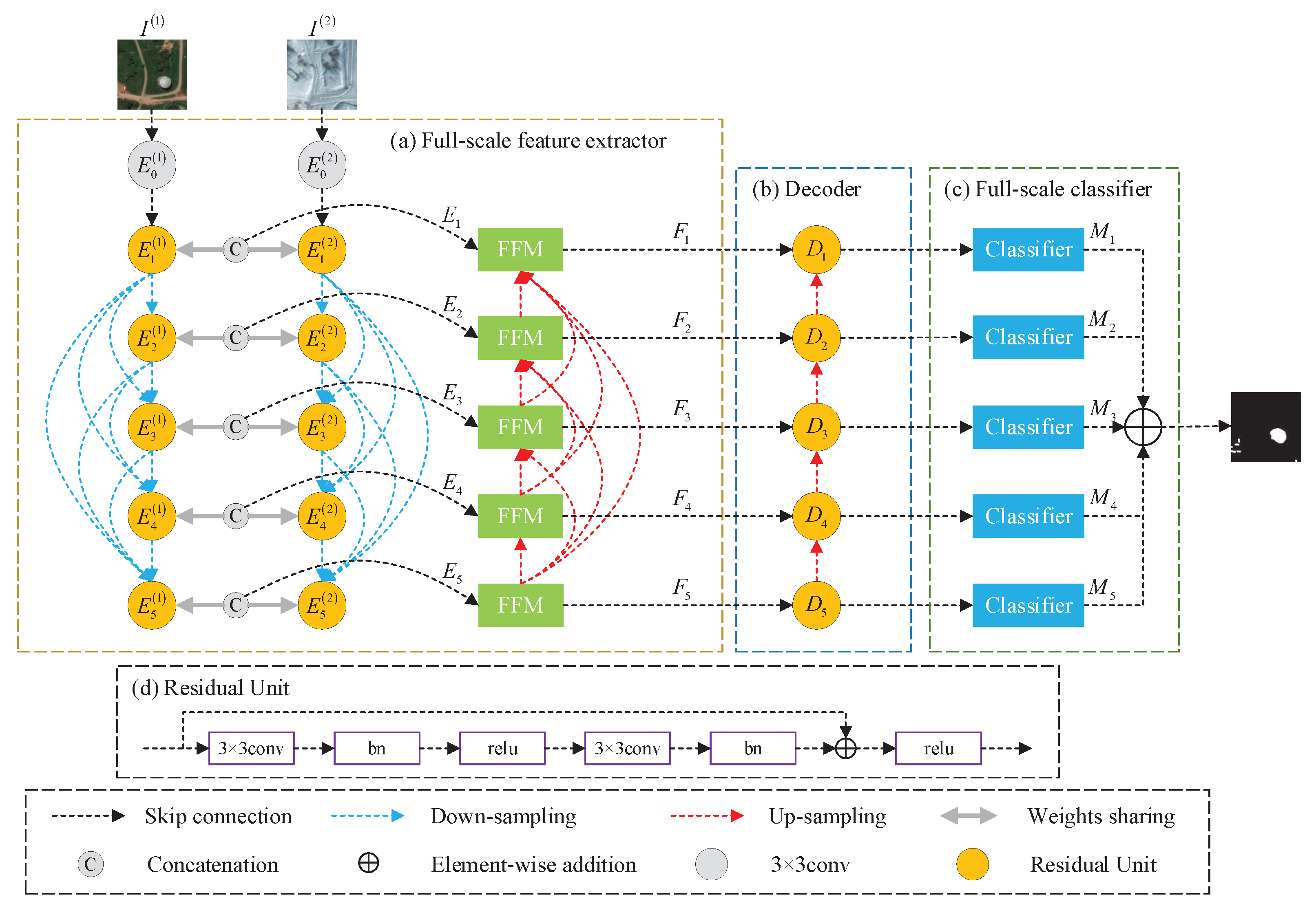
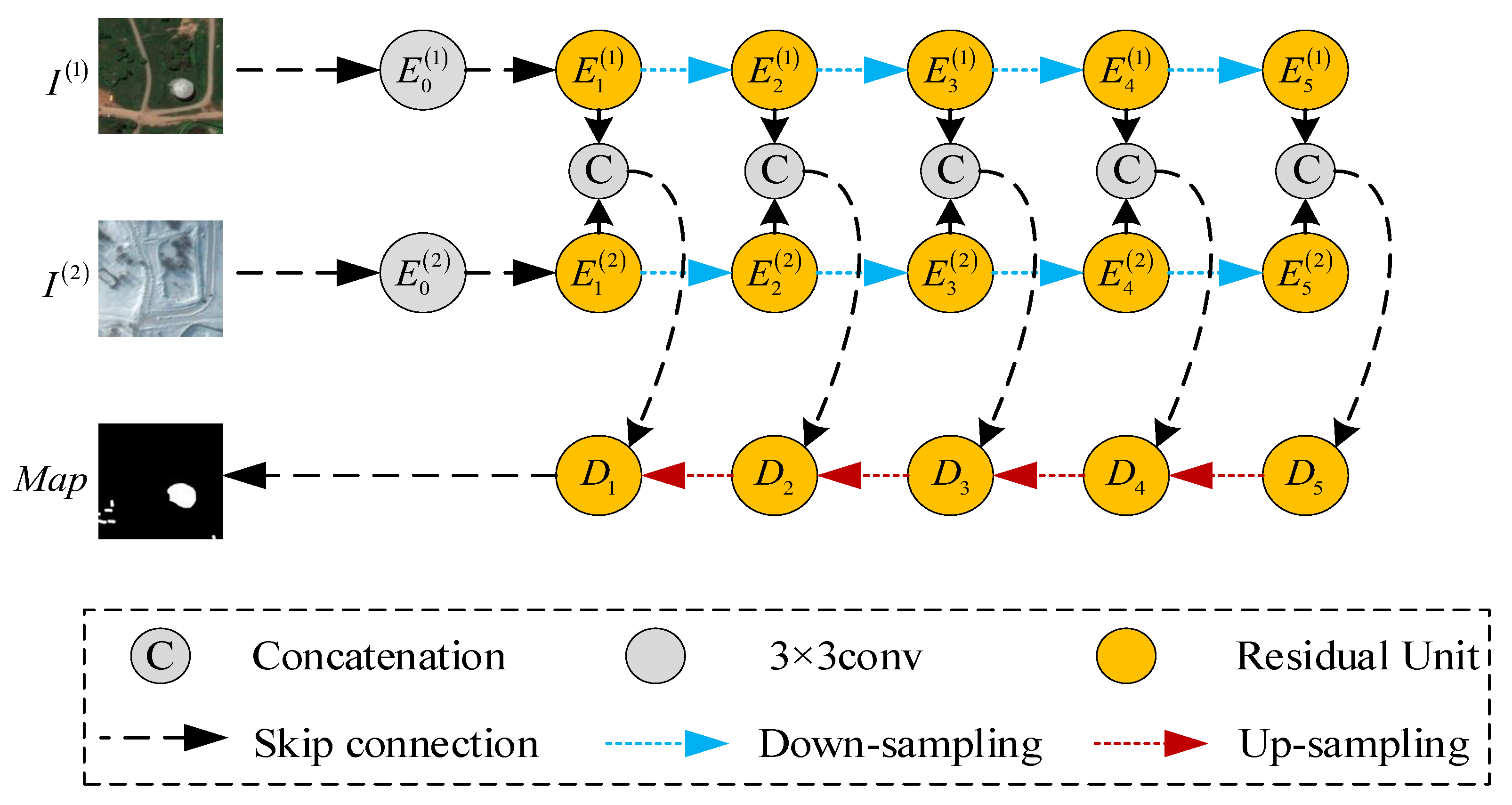
2.1. Full-Scale Feature Extractor (FFE)

In the plain networks, the spatial localization of deep features becomes less precise with successive down-sampling, which is detrimental to the detection of small objects and object edges; while shallow features lack sufficient change semantics, which affects the detection performance of the network in complex scenes. To obtain feature maps with accurate localization and rich semantics, a full-scale feature extractor is designed to explore the information of feature maps from full scales fully. As shown in Figure 2a, the full-scale feature extractor is used as an encoder, which contains a top-down branch and a bottom-up branch.

The top-down branch is a two-stream architecture with shared weights to independently encode the deep features of the bi-temporal images. To enhance the spatial localization of deep features, we enable the deep layer to receive all shallower feature maps directly through dense top-down skip connections. To achieve this, when small-scale feature maps from shallow layers are delivered to deeper layers, their scales are restored to the same as the large-scale feature maps by max-pooling, and then all feature maps mapped to the same layer are concatenated.

We set a hyperparameter C to adjust the width (the number of channels of the feature map) of all feature maps in the network. In the top-down branch, the main body of the branch contains five stages: the first stage contains a 3 × 3 convolution layer and a residual unit, which changes the feature map width to C; while the 2nd, 3rd, 4th, and 5th stages all contain only a down-sampling layer and a residual unit, and the widths of the feature maps they output are 2C, 4C, 8C, and 16C, respectively. $\left\{E_i^{\left(N\right)}\mid i=1,2,3,4,5;N=1,2\right\}$ denotes the set of feature maps extracted from the top-down branch, i is layer indexes, N represents the two streams of the branch, the stack of feature maps represented by $E_i^{\left(N\right)}$ can be represented as:

$$E_i^{\left(N\right)}{E}_i^{\left(N\right)}=\left\{\begin{array}{cc}{C}_R\left(C_{3\times 3}\left(I^{\left(N\right)}\right)\right),\hfill & i=1\hfill \\ C_R\left(\left[D{\left(E_k^{\left(N\right)}\right)}_{k=1}^{i-1}\right]\right),\hfill & i=2,3,4,5\hfill \end{array}\right.$$

(1)

where $I^{\left(N\right)}$ denotes the bi-temporal images, function $I^{\left(N\right)}{C}_{3\times 3}(•)$ denotes a $3\times 3$ convolution layer followed by a batch normalization and a ReLU function. $C_R(•)$ denotes the residual unit, as shown in Figure 2d, $D(·)$ indicates down-sampling (max pooling), and $[·]$ represents the concatenation.

To achieve information interaction, feature maps of the same scale for the two streams in the top-down branch are concatenated. $\left\{E_i\mid i=1,2,3,4,5\right\}$ denotes the set of the concatenated feature maps, i is layer indexes, then $E_i$ can be represented as:

$$E_i=\left[E_i^{\left(1\right)},E_i^{\left(2\right)}\right],i=1,2,3,4,5$$

(2)

where $E_i^{\left(1\right)}$ and $E_i^{\left(2\right)}$ denote the feature maps output by the two streams in the top-down branch, respectively.

The bottom-up branch allows the shallow layer to directly receive all the feature maps from the deeper layers through dense bottom-up skip connections, thus delivering the high-level semantics from the deeper layers to the shallow layers. As shown in Figure 5, the feature fusion module (FFM) receives both feature maps of the same scale from the top-down branch and all feature maps of larger scale from the bottom-up branch, and finally generates $F_i$. Specifically, $E_i$ is fed into a $1\times 1$ convolution layer to reduce its width (in our experiments, the width of $E_i$ is halved). Meanwhile, the larger scale feature maps from the bottom-up branch, $F_{i+1},\dots ,F_5$ are fed into the $1\times 1$ convolution layer followed by a bilinear up-sampling. For simplicity, when $F_j$ is delivered to $F_i$, (i,j are layer index, $j>i$), the width of $F_j$ is reduced to be the same as $F_i$ by the $1\times 1$ convolution. Finally, feature maps mapped to the same layer are concatenated and then an additional $1\times 1$ convolution is used to achieve cross-channel fusion of the aggregated feature maps. We specify the widths for $F_1,F_2,F_3,F_4$ and $F_5$ as C, 2C, 4C, 8C, and 16C, respectively. $\left\{F_i\mid i=1,2,3,4,5\right\}$ denotes the set of feature maps extracted from the bottom-up branch, i is layer indexes, then $F_i$ can be represented as:

$$F_i=\left\{\begin{array}{cc}C\left(E_5\right),\hfill & i=5\hfill \\ C\left(\left[C\left(E_i\right),U{\left(C\left(F_j\right)\right)}_{j=i+1}^5\right]\right),\hfill & i=1,2,3,4\hfill \end{array}\right.$$

(3)

where function $C(·)$ denotes a $1\times 1$ convolution, $U(·)$ indicates bilinear up-sampling, and $[·]$ represents the concatenation.

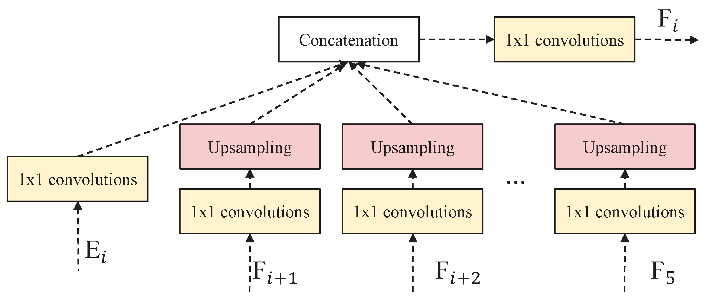
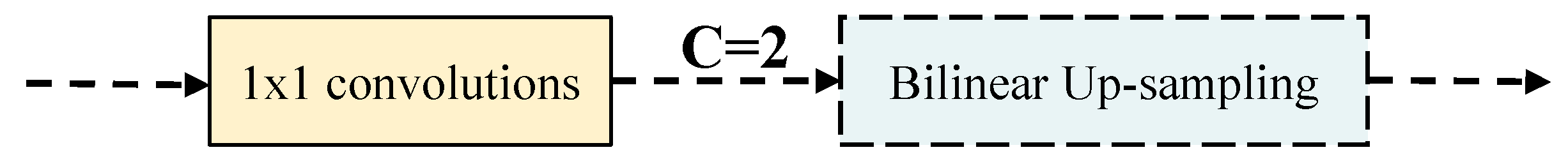
2.2. Decoder and Full-Scale Classifier (FC)

The decoder consists of multiple residual units and deconvolution blocks. Through the decoder, the network extracts the changing semantics between the bi-temporal images and generates multi-scale feature maps, i.e., $D_1,D_2,D_3,D_4$ and $D_5$.

To further exploit these feature maps, we propose a full-scale classifier that combines feature maps from all scales of the decoder for classification with marginal extra cost. Specifically, the full-scale classifier consists of five lightweight classifiers that correspond to five feature maps of different scales of the decoder. For simplicity, each classifier consists of a 1 × 1 convolutional layer followed by a bilinear up-sampling ($D_1$ is not upsampled). As shown in Figure 6, the feature map is first reduced to 2 channels (change or unchanged) by the $1\times 1$ convolution, then upsampled to the same scale as the original images. Finally, the prediction maps generated by these five classifiers are merged by element-wise addition. Then, the full-scale classifier can be calculated as follows:

$$M_i=C\left(D_1\right)\mathrm{if}i=1\mathrm{else}U\left(C\left(D_i\right)\right)$$

(4)

$$\mathrm{Map}=\sum _{i=1}^5{M}_i$$

(5)

where $M_i$ denotes the prediction maps generated by each layer of the decoder. The function $C(·)$ denotes a $1\times 1$ convolution, $U(·)$ indicates bilinear up-sampling. Compared with the full-scale deep supervision in UNet3+ [37] and IFN [26], F3SNet incorporates prediction maps of different scales generated by full-scale deep supervision and thus learns the hierarchical representations of the change maps, which further improves the network’s robustness to object scale variations. As these prediction maps are obtained with learnable parameters, the network can adaptively adjust the weights for each scale, assigning larger weights to important scales and smaller weights to less important scales.

3. Experiments

3.1. Data Set

We have conducted a series of experiments on two large-scale public CD datasets.

CDD [45] dataset is obtained by cropping and rotating 7 pairs of season-varying images with the resolution of 4725 × 2700 pixels and 4 season-varying image pairs with minimal changes and the resolution of 1900 × 1000 pixels. The dataset contains 16,000 image sets with image size 256 × 256 pixels, including 10,000 train sets and 3000 test and validation sets with a spatial resolution of 3100 cm/px.

LEVIR-CD [34] contains 637 pairs of very high-resolution (50 cm/px) remote sensing images with an image size of 1024 × 1024 pixels. We follow its default dataset allocation. Due to the limitation of GPU memory capacity, we split each image into 16 small patches of size 256 × 256 pixels without overlapping. After image slicing, the number of image pairs in the training set, validation set and test set are 7120, 1024 and 2048, respectively.

3.2. Metrics and Implementation Details

Our F3SNet uses the plain cross-entropy loss function without pre-training. In the training phase, Adam is used as the optimizer, the learning rate is set to 0.005, and the batch size is set to 16. The weights of each convolutional layer are initialized by KaiMing normalization. The proposed method is implemented by PyTorch, and powered by an NVIDIA Tesla v100, which converges in 100 epochs. To evaluate the performance of the F3SNet, four evaluation indicators are used: Precision (Pre), Recall (Rec), F1-score (F1), and Intersection over Union (IoU). They are calculated as follows:

$$\mathrm{Pre}=tp/(tp+fp)$$

(6)

$$\mathrm{Rec}=tp/(tp+fn)$$

(7)

$$\mathrm{F}1=2Pre\ast Rec/(\mathrm{Pre}+Rec)$$

(8)

$$\mathrm{IOU}=tp/(fp+tp+fn)$$

(9)

where $tp$, $fp$, $fn$ is the number of true positives, false positives and false negatives, respectively.

3.3. Experimental Results

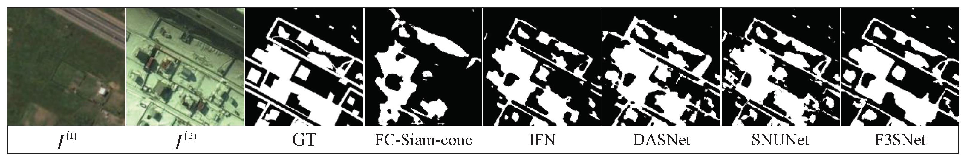
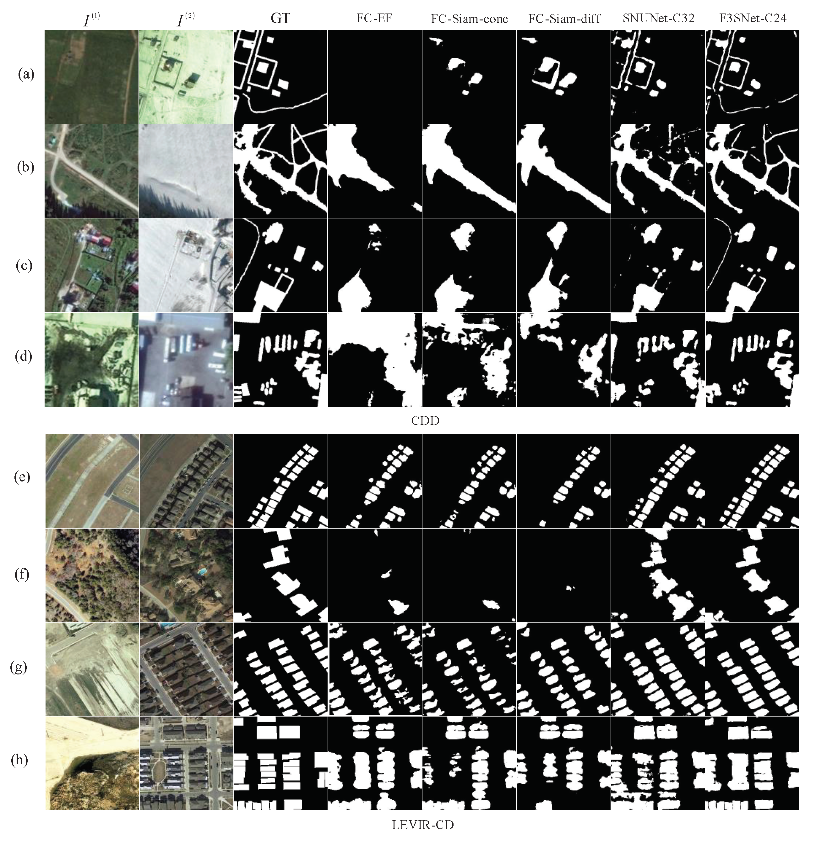
3.3.1. Comparison with Other Methods

We have compared some state-of-the-art change detection methods:

• FC-EF [25]: The EF architecture concatenates bi-temporal images as different color channels and feeds them into a convolutional neural network.
• FC-Siam-conc [25]: A combination of siamese networks and UNet. The deep features of the raw image are extracted by the two-stream encoder and then fed into the decoder to extract the change semantic information further.
• FC-Siam-diff [25]: Deep features of the raw images are extracted by a siamese network, and the feature differences are fed into the decoder.
• IFN [26]: The pre-trained VGG-16 is used as a branch of the two-stream encoder, and the attention module is used to guide a better fusion of the feature maps of the encoder and decoder.
• DASNet [33]: Through the dual-attention mechanism, long-range dependencies are captured to obtain more discriminative feature representations.
• STANet [34]: A siamese-based spatial-temporal attention neural network, which partitions the image into multi-scale subregions and introduces self-attention into all sub-regions.
• SNUNet [30]: A combination of the Siamese network and the NestedUNet, which alleviates the loss of localization information in deeper layers by reusing shallow features.

In order to adapt to different CD tasks to achieve a better balance between performance and efficiency, we can adjust the overall number of parameters of the network by adjusting the hyperparameter C. From

Table 1. Comparison results on the two CD test sets. The highest scores are marked in bold. The size of the input image for the model is 256 × 256 × 3 to calculate GFLOPs.

Methods	FLOPs (G)	CDD				LEVIR-CD
		Pre	Rec	F1	IoU	Pre	Rec	F1	IoU
FC-EF	7.14	0.749	0.494	0.595	0.423	0.754	0.730	0.742	0.590
FC-Siam-con	10.64	0.779	0.622	0.692	0.529	0.852	0.736	0.790	0.653
FC-Siam-diff	9.44	0.786	0.588	0.673	0.507	0.861	0.687	0.764	0.618
IFN	164.58	0.950	0.861	0.903	0.823	0.903	0.876	0.889	0.800
STANet	25.76	0.863	0.760	0.787	0.649	0.838	0.910	0.873	0.775
DASNet	113.09	0.914	0.925	0.919	0.850	0.811	0.788	0.799	0.665
SNUNet	109.62	0.956	0.949	0.953	0.910	0.889	0.874	0.881	0.787
F3SNet/8	3.24	0.952	0.907	0.929	0.867	0.913	0.898	0.905	0.826
F3SNet/16	12.56	0.964	0.944	0.954	0.912	0.917	0.897	0.907	0.830
F3SNet/24	27.98	0.967	0.964	0.966	0.934	0.907	0.908	0.907	0.830
F3SNet/32	49.49	0.970	0.965	0.968	0.938	0.919	0.900	0.909	0.833

and

Table 2. Time performances of different methods.

Method	FC-EF	IFN	DASNet	SNUNet	F3SNet/8	F3SNet/32
Train Time (s/epoch)	179	1218	926	745	133	546
Testing Time (s)	31	84	79	70	32	55
Parameters (M)	1.35	35.72	16.25	12.03	0.97	15.77

, we can observe that F3SNet significantly outperforms other CD methods when the number of parameters or floating point operations of the network is close. Specifically, on the CDD dataset, when C = 24, F3SNet achieves 0.967, 0.964, 0.966, and 0.934 for precision, recall, F1-score, and IoU, respectively, using only 8.87M number of parameters and 27.98G floating-point operations. On the LEVIR-VD dataset, when C = 8, F3SNet’s F1-score is 0.905, which is also significantly better than other networks. It is worth noting that the number of parameters and floating-point operations of F3SNet only account for 7.5% and 3.0% of the SNUNet, respectively.

To evaluate the performance of F3SNet more intuitively, we visualize some experimental results from the CDD test set and the LEVIR-CD test set. From Figure 1 and Figure 7, we can observe that there are seasonal variations in Figure 1 and Figure 7a–c, and significant illumination variations in Figure 7d–h. In these samples, FC-EF, FC-Siam-conc, FC-Siam-diff can only detect rough outlines of change objects, while IFN and SNUNet still have difficulty in accurately identifying some small or elongated objects. In contrast, F3SNet can segment these change objects more completely and maintain high performance even in complex scenes. These performance improvements can be attributed to the full-scale feature fusion and the combination of full-scale prediction maps.

In addition, Table 2 shows the training time and test time for 30,000 pairs of images of size 256 × 256 pixels. For a fair comparison, we adopt the same batch size (16) for all the experiments. According to Table 2, our 8-channel F3SNet shows better time performance, while the 32-channel F3SNet also achieves competitive results. In practical applications, a network with the right number of channels can be chosen according to specific needs.

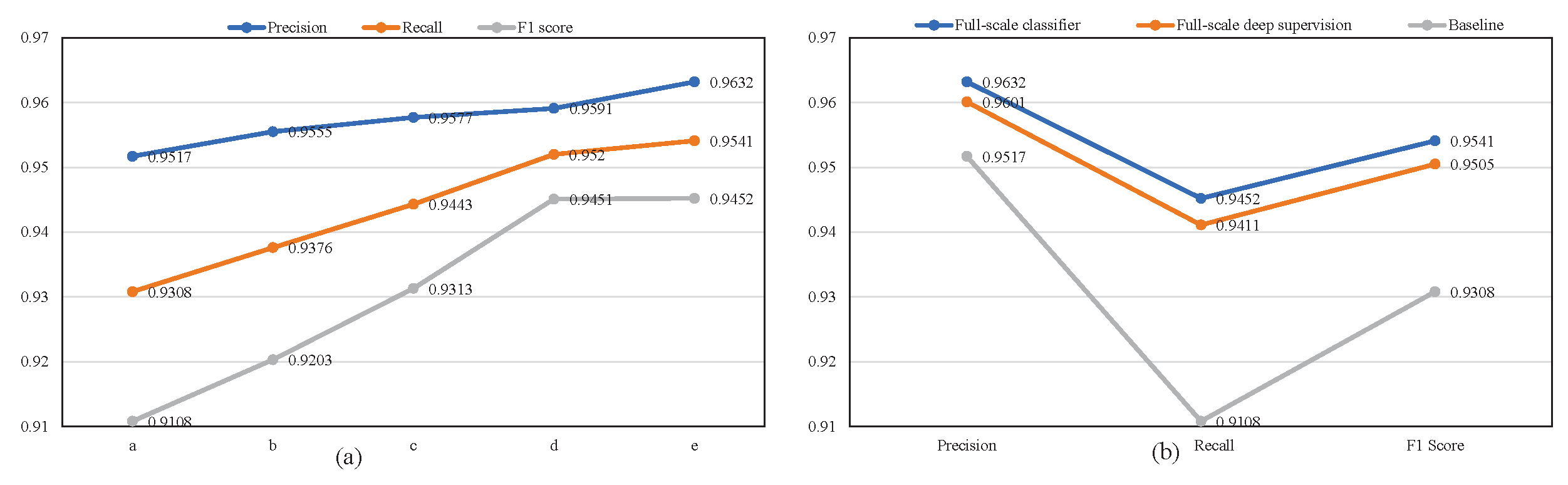
3.3.2. Ablation Study for Full-Scale Feature Extractor (FFE) and Full-Scale Classifier (FC)

To quantify the performance gains of FFE and FC, their ablation results are listed in

Table 3. Ablation results of full-scale feature extractors (FFE) and full-scale classifiers (FC) on the CDD test set (C = 32). When FFE and FC are not used, we use the plain siamese network (Figure 7).

Index	FFE	FC	Par (M)	GFLOPs	Pre	Rec	F1	IOU
1			13.54	43.89	0.9517	0.9108	0.9308	0.8706
2	✓		15.76	49.47	0.9665	0.9530	0.9597	0.9225
3		✓	13.55	43.91	0.9632	0.9452	0.9541	0.9123
4	✓	✓	15.77	49.49	0.9701	0.9657	0.9679	0.9378

. All the experiments use the same hyperparameters. We can observe that both the full-scale feature extractor and the full-scale classifier improve network performance comprehensively compared to the baseline network. Specifically, the FFE and FC improve the F1-score by 2.89% and 2.33%, respectively, and by 3.71% in combination. In addition, its number of parameters and floating point operations increased by a total of only 2.23 M and 5.60 GFLPOs, achieving a good trade-off between accuracy and efficiency.

Although the full-scale feature extractor uses the densest skip connections, its number of parameters and floating-point operations only increase by 2.22 M and 5.58 GFLPOs compared to the baseline network (Figure 8), which is since we use a large number of 1 × 1 convolutions to reduce the number of channels of the feature maps. In addition, our full-scale classifier brings significant performance gains with marginal extra cost, which can be attributed to the following two reasons: (i) the network is more fully trained through full-scale deep supervision; and (ii) the robustness of the network to object scale variations is improved through the combination of full-scale prediction maps.

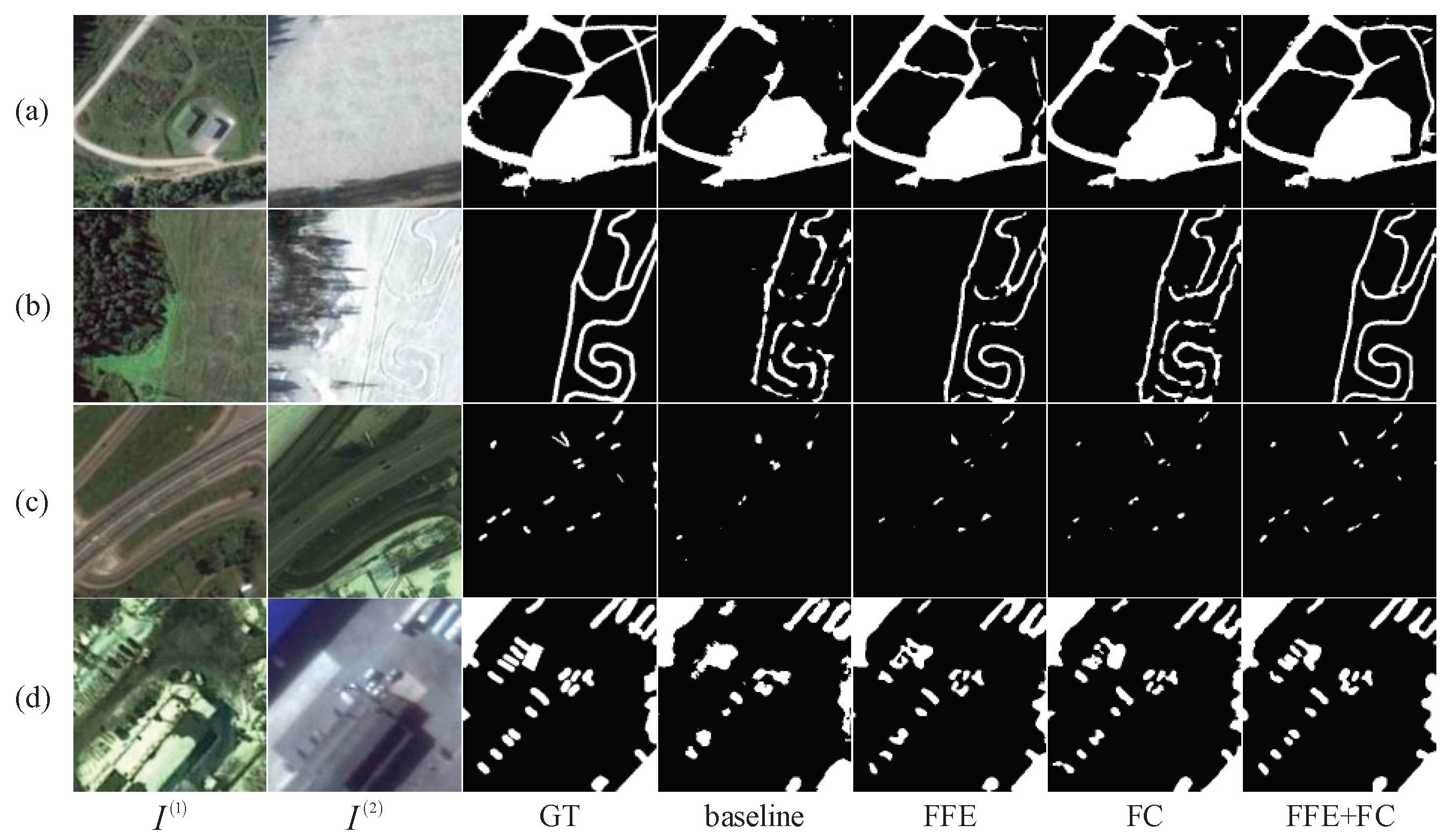
3.3.3. Visualization of FFE and FC Effect

To more intuitively reflect the specific role played by these two modules, we visualized these four networks corresponding to Table 3. In Figure 9, there is a significant environmental variation (seasonal changes, illumination changes) between the bi-temporal images. We can observe that the baseline network cannot completely segment the change objects, especially the objects edges and slender objects. In addition to this, some small objects are missed.

From Figure 9a,b,d, we can observe that FFE can segment the object edges and slender objects more clearly; while from Figure 9c, we can observe that FC can identify small objects better. When these two modules are combined, the segmentation performance of both small objects and object edges is further improved.

According to Table 3 and Figure 9, we can infer that FFE and FC do not play exactly the same role in the network. When these two modules are used together, they can complement each other in terms of information.

3.3.4. Comparison with Wider Baseline

We appropriately increase the number of channels in the baseline network so that the number of parameters is not less than our proposed network. According to

Table 4. Comparison of the baseline network (Figure 6), the wide baseline network, and our proposed method (using only FFE).

Model	Channels	Params (M)	Pre	Rec	F1	IOU
baseline	32	13.54	0.9517	0.9108	0.9308	0.8706
baseline	35	16.20	0.9558	0.9109	0.9328	0.8741
baseline	32	15.76	0.9665	0.9530	0.9597	0.9225

, the wide baseline network outperforms the baseline network due to the higher number of parameters in the wide baseline network.

When using only the full-scale feature extractor, our F3SNet outperforms the baseline network by 1.48%, 4.22%, 2.89% and 0.519% in terms of precision, recall, F1-score and IoU, respectively, and by 1.07%, 4.21%, 2.69% and 4.84% over the wide baseline network, respectively, indicating that the performance gain from the full-scale feature extractor relies mainly on the improvement of the network architecture rather than the increase of the number of parameters.

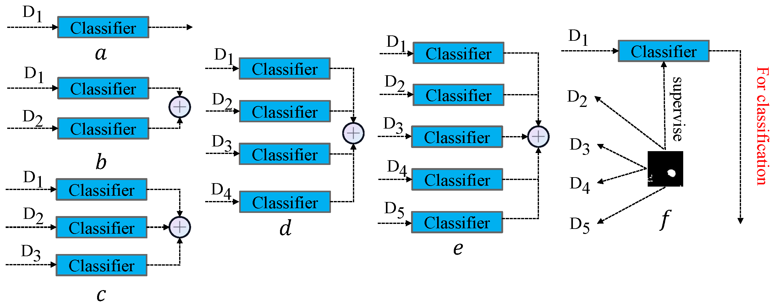
3.3.5. Evaluation of Full-Scale Classifiers

For the multi-scale feature maps generated by the decoder, we compared several different fusion methods to verify the effectiveness of full-scale prediction map fusion. As shown in Figure 3a–e represent different fusion methods of the decoder feature maps. Intuitively, e incorporates more prediction maps and thus allows for more sufficient training of the feature maps in the intermediate layer as well as more effective improvement of the network’s robustness to object scale variations. According to Figure 4a, the more feature maps of different scales the classifier combines, the higher the performance of the network, which supports our speculation.

To further explore why the full classifier works, we replace the full-scale classifier with full-scale deep supervision to eliminate the effect of combining full-scale prediction maps. As shown in Figure 3f, the full-scale feature maps of the decoder are supervised by ground truth and ultimately use only $D_1$ for classification. To achieve deep supervision, each side output of the decoder is fed into a 1 × 1 convolution layer followed by a bilinear up-sampling.

According to Figure 4b, full-scale deep supervision significantly improves the network performance, which indicates that one of the roles of the full-scale classifier is deep supervision. On the other hand, compared to full-scale deep supervision, the full-scale classifier improves the precision, recall, and F1-score of the network by 0.31%, 0.41%, and 0.36%, respectively, and these improvements can be attributed to the fusion of the full-scale prediction maps. Overall, the primary role of the full-scale classifier is to train the feature maps in the intermediate layer more fully, and the secondary role is to fuse the full-scale prediction maps.

4. Conclusions

In this paper, we propose a full-scale feature fusion siamese network (F3SNet) for remote sensing change detection, which takes full advantage of different scale feature maps through full-scale feature fusion and full-scale prediction. Full-scale feature fusion enhances the spatial localization of deep features and complements the changing semantics of shallow features through dense skip connections; while full-scale prediction can train the feature maps of intermediate layers more sufficiently, it improves the robustness to object scale variations by fusing full-scale prediction maps. Compared with other methods, F3SNet significantly improves the detection performance for small objects and object edges and maintains high performance even in complex scenes.

References

1. Eismann, M.T.; Meola, J.; Hardie, R.C. Hyperspectral Change Detection in the Presenceof Diurnal and Seasonal Variations. IEEE Trans. Geosci. Remote Sens. 2008, 46, 237–249. [Google Scholar] [CrossRef]
2. Choi, E.; Kim, J. Robust Change Detection Using Channel-Wise co-Attention-Based Siamese Network With Contrastive Loss Function. IEEE Access 2022, 10, 45365–45374. [Google Scholar] [CrossRef]
3. Zhou, Y.; Feng, Y.; Huo, S.; Li, X. Joint Frequency-Spatial Domain Network for Remote Sensing Optical Image Change Detection. IEEE Trans. Geosci. Remote Sens. 2022, 60, 5627114. [Google Scholar] [CrossRef]
4. Nagatani, I.; Hayashi, M.; Watanabe, M.; Tadono, T.; Watanabe, T.; Koyama, C.; Shimada, M. Seasonal Change Analysis for ALOS-2 PALSAR-2 Deforestation Detection. In Proceedings of the IGARSS 2020–2020 IEEE International Geoscience and Remote Sensing Symposium, Waikoloa, HI, USA, 26 September–2 October 2020; pp. 3807–3810. [Google Scholar]
5. Zhang, J.; Pan, B.; Zhang, Y.; Liu, Z.; Zheng, X. Building Change Detection in Remote Sensing Images Based on Dual Multi-Scale Attention. Remote Sens. 2022, 14, 5405. [Google Scholar] [CrossRef]
6. Jiang, J.; Xiang, J.; Yan, E.; Song, Y.; Mo, D. Forest-CD: Forest Change Detection Network Based on VHR Images. IEEE Geosci. Remote. Sens. Lett. 2022, 19, 2506005. [Google Scholar] [CrossRef]
7. Li, L.; Ma, H.; Jia, Z. Multiscale geometric analysis fusion-based unsupervised change detection in remote sensing images via FLICM Model. Entropy 2022, 24, 291. [Google Scholar] [CrossRef]
8. Arjasakusuma, S.; Kusuma, S.S.; Melati, P.; Hafiudzan, A. Change Detection Analysis using Bitemporal PRISMA Hyperspectral Data: Case Study of Magelang and Boyolali Districts, Central Java Province, Indonesia. J. Indian Soc. Remote. Sens. 2022, 50, 1803–1811. [Google Scholar] [CrossRef]
9. Soto, P.J.; Costa, G.A.; Feitosa, R.Q.; Ortega, M.X.; Bermudez, J.D.; Turnes, J.N. Domain-Adversarial Neural Networks for Deforestation Detection in Tropical Forests. IEEE Geosci. Remote Sens. Lett. 2022, 19, 2504505. [Google Scholar] [CrossRef]
10. Marinelli, D.; Coops, N.C.; Bolton, D.K.; Bruzzone, L. An unsupervised change detection method for lidar data in forest areas based on change vector analysis in the polar domain. In Proceedings of the IGARSS 2018—2018 IEEE International Geoscience and Remote Sensing Symposium, Valencia, Spain, 22–27 July 2018; pp. 1922–1925. [Google Scholar]
11. Verma, H.C.; Ahmed, T.; Rajan, S.; Hasan, M.K.; Khan, A.; Gohel, H.; Adam, A. Development of LR-PCA Based Fusion Approach to Detect the Changes in Mango Fruit Crop by Using Landsat 8 OLI Images. IEEE Access 2022, 10, 85764–85776. [Google Scholar] [CrossRef]
12. Sadeghi, V.; Etemadfard, H. Optimal cluster number determination of FCM for unsupervised change detection in remote sensing images. Earth Sci. Inform. 2022, 15, 1045–1057. [Google Scholar] [CrossRef]
13. Martinez-Izquierdo, M.d.E.; Molina-Sánchez, I.; Morillo-Balsera, M.d.C. Efficient Dimensionality Reduction using Principal Component Analysis for Image Change Detection. IEEE Lat. Am. Trans. 2019, 17, 540–547. [Google Scholar] [CrossRef]
14. Toure, S.; Diop, O.; Kpalma, K.; Maiga, A.S. Shoreline Detection using Optical Remote Sensing: A Review. ISPRS Int. J. Geo-Inf. 2019, 8, 75. [Google Scholar] [CrossRef] [Green Version]
15. Han, T.; Wulder, M.A.; White, J.C.; Coops, N.C.; Alvarez, M.F.; Butson, C. An Efficient Protocol to Process Landsat Images for Change Detection With Tasselled Cap Transformation. IEEE Geosci. Remote Sens. Lett. 2007, 4, 147–151. [Google Scholar] [CrossRef]
16. Gong, M.; Yang, H.; Zhang, P. Feature learning and change feature classification based on deep learning for ternary change detection in SAR images. ISPRS J. Photogramm. Remote Sens. 2017, 129, 212–225. [Google Scholar] [CrossRef]
17. Grinblat, G.L.; Uzal, L.C.; Granitto, P.M. Abrupt change detection with One-Class Time-Adaptive Support Vector Machines. Expert Syst. Appl. 2013, 40, 7242–7249. [Google Scholar] [CrossRef] [Green Version]
18. Fanara, L.; Gwinner, K.; Hauber, E.; Oberst, J. Automated detection of block falls in the north polar region of Mars. Planet. Space Sci. 2020, 180, 104733. [Google Scholar] [CrossRef]
19. Ronneberger, O.; Fischer, P.; Brox, T. U-Net: Convolutional Networks for Biomedical Image Segmentation. In Proceedings of the Medical Image Computing and Computer-Assisted Intervention, Munich, Germany, 5–9 October 2015; Springer: Cham, Switzerland, 2015; pp. 234–241. [Google Scholar]
20. Lv, Z.; Wang, F.; Cui, G.; Benediktsson, J.A.; Lei, T.; Sun, W. Spatial–Spectral Attention Network Guided with Change Magnitude Image for Land Cover Change Detection Using Remote Sensing Images. IEEE Trans. Geosci. Remote Sens. 2022, 60, 4412712. [Google Scholar] [CrossRef]
21. Zheng, H.; Gong, M.; Liu, T.; Jiang, F.; Zhan, T.; Lu, D.; Zhang, M. HFA-Net: High frequency attention siamese network for building change detection in VHR remote sensing images. Pattern Recognit. 2022, 129, 108717. [Google Scholar] [CrossRef]
22. Zhou, Z.; Rahman Siddiquee, M.M.; Tajbakhsh, N.; Liang, J. UNet++: A Nested U-Net Architecture for Medical Image Segmentation. In Deep Learning in Medical Image Analysis and Multimodal Learning for Clinical Decision Support; Springer International Publishing: Cham, Switzerland, 2018; pp. 3–11. [Google Scholar]
23. Raza, A.; Huo, H.; Fang, T. EUNet-CD: Efficient UNet++ for Change Detection of Very High-Resolution Remote Sensing Images. IEEE Geosci. Remote Sens. Lett. 2022, 19, 3510805. [Google Scholar] [CrossRef]
24. Peng, X.; Zhong, R.; Li, Z.; Li, Q. Optical Remote Sensing Image Change Detection Based on Attention Mechanism and Image Difference. IEEE Trans. Geosci. Remote Sens. 2021, 59, 7296–7307. [Google Scholar] [CrossRef]
25. Caye Daudt, R.; Le Saux, B.; Boulch, A. Fully Convolutional Siamese Networks for Change Detection. In Proceedings of the 2018 25th IEEE International Conference on Image Processing (ICIP), Athens, Greece, 7–10 October 2018; pp. 4063–4067. [Google Scholar]
26. Zhang, C.; Yue, P.; Tapete, D.; Jiang, L.; Shangguan, B.; Huang, L.; Liu, G. A deeply supervised image fusion network for change detection in high resolution bi-temporal remote sensing images. ISPRS J. Photogramm. Remote Sens. 2020, 166, 183–200. [Google Scholar] [CrossRef]
27. Ji, S.; Wei, S.; Lu, M. Fully Convolutional Networks for Multisource Building Extraction From an Open Aerial and Satellite Imagery Data Set. IEEE Trans. Geosci. Remote Sens. 2019, 57, 574–586. [Google Scholar] [CrossRef]
28. Bao, T.; Fu, C.; Fang, T.; Huo, H. PPCNET: A Combined Patch-Level and Pixel-Level End-to-End Deep Network for High-Resolution Remote Sensing Image Change Detection. IEEE Geosci. Remote Sens. Lett. 2020, 17, 1797–1801. [Google Scholar] [CrossRef]
29. Yu, B.; Chen, F.; Wang, Y.; Wang, N.; Yang, X.; Ma, P.; Zhou, C.; Zhang, Y. Res2-Unet+, a Practical Oil Tank Detection Network for Large-Scale High Spatial Resolution Images. Remote Sens. 2021, 13, 4740. [Google Scholar] [CrossRef]
30. Fang, S.; Li, K.; Shao, J.; Li, Z. SNUNet-CD: A Densely Connected Siamese Network for Change Detection of VHR Images. IEEE Geosci. Remote Sens. Lett. 2021, 19, 8007805. [Google Scholar] [CrossRef]
31. Li, X.; Du, Z.; Huang, Y.; Tan, Z. A deep translation (GAN) based change detection network for optical and SAR remote sensing images. ISPRS J. Photogramm. Remote Sens. 2021, 179, 14–34. [Google Scholar] [CrossRef]
32. Chen, Z.; Zhou, Y.; Wang, B.; Xu, X.; He, N.; Jin, S.; Jin, S. EGDE-Net: A building change detection method for high-resolution remote sensing imagery based on edge guidance and differential enhancement. ISPRS J. Photogramm. Remote Sens. 2022, 191, 203–222. [Google Scholar] [CrossRef]
33. Chen, J.; Yuan, Z.; Peng, J.; Chen, L.; Huang, H.; Zhu, J.; Liu, Y.; Li, H. DASNet: Dual Attentive Fully Convolutional Siamese Networks for Change Detection in High-Resolution Satellite Images. IEEE J. Sel. Top. Appl. Earth Obs. Remote Sens. 2021, 14, 1194–1206. [Google Scholar] [CrossRef]
34. Chen, H.; Shi, Z. A spatial-temporal attention-based method and a new dataset for remote sensing image change detection. Remote Sens. 2020, 12, 1662. [Google Scholar] [CrossRef]
35. Fu, J.; Liu, J.; Tian, H.; Li, Y.; Bao, Y.; Fang, Z.; Lu, H. Dual Attention Network for Scene Segmentation. In Proceedings of the 2019 IEEE/CVF Conference on Computer Vision and Pattern Recognition (CVPR), Long Beach, CA, USA, 16–17 June 2019; pp. 3141–3149. [Google Scholar]
36. Zhou, T.; Wang, S.; Zhou, Y.; Yao, Y.; Li, J.; Shao, L. Motion-Attentive Transition for Zero-Shot Video Object Segmentation. In Proceedings of the AAAI Conference on Artificial Intelligence, New York, NY, USA, 7–12 February 2020; Volume 34, pp. 13066–13073. [Google Scholar]
37. Song, A.; Choi, J.; Han, Y.; Kim, Y. Change Detection in Hyperspectral Images Using Recurrent 3D Fully Convolutional Networks. Remote Sens. 2018, 10, 1827. [Google Scholar] [CrossRef]
38. Ibtehaz, N.; Rahman, M.S. MultiResUNet: Rethinking the U-Net architecture for multimodal biomedical image segmentation. Neural Networks 2020, 121, 74–87. [Google Scholar] [CrossRef] [PubMed]
39. Lebedev, M.; Vizilter, Y.V.; Vygolov, O.; Knyaz, V.; Rubis, A.Y. Change detection in remote sensing images using conditional adversarial networks. Int. Arch. Photogramm. Remote Sens. Spat. Inf. Sci. 2018, 42, 565–571. [Google Scholar] [CrossRef] [Green Version]
40. He, H.; Chen, Y.; Li, M.; Chen, Q. ForkNet: Strong Semantic Feature Representation and Subregion Supervision for Accurate Remote Sensing Change Detection. IEEE J. Sel. Top. Appl. Earth Obs. Remote Sens. 2022, 15, 2142–2153. [Google Scholar] [CrossRef]
41. Wang, J.; Sun, K.; Cheng, T.; Jiang, B.; Deng, C.; Zhao, Y.; Liu, D.; Mu, Y.; Tan, M.; Wang, X.; et al. Deep High-Resolution Representation Learning for Visual Recognition. IEEE Trans. Pattern Anal. Mach. Intell. 2021, 43, 3349–3364. [Google Scholar] [CrossRef]
42. Lal, S.; Nalini, J.; Reddy, C.S. DIResUNet: Architecture for multiclass semantic segmentation of high resolution remote sensing imagery data. Appl. Intell. 2022, 52, 15462–15482. [Google Scholar]
43. Zhou, R.H.M.; Xing, Y.; Zou, Y.; Fan, W. Change detection with various combinations of fluid pyramid integration networks. Neurocomputing 2021, 437, 84–94. [Google Scholar]
44. Xu, J.; Luo, Y.; Chen, X.; Luo, C. An Adaptive Multi-Scale and Multi-Level Features Fusion Network with Perceptual Loss for Change Detection. In Proceedings of the ICASSP 2021–2021 IEEE International Conference on Acoustics, Speech and Signal Processing (ICASSP), Toronto, ON, Canada, 6–11 June 2021; pp. 2275–2279. [Google Scholar]
45. Chen, H.; Wu, C.; Du, B.; Zhang, L. Deep Siamese Multi-scale Convolutional Network for Change Detection in Multi-temporal VHR Images. In Proceedings of the 2019 10th International Workshop on the Analysis of Multitemporal Remote Sensing Images (MultiTemp), Shanghai, China, 5–7 August 2019; pp. 1–4. [Google Scholar]
Figure 1. Visualization results of the different methods on the CDD [39] test set. I ( 1 ) and I ( 2 ) are the bi-temporal images, GT is ground truth. FC-Siam-conc [25], IFN [26], DASNet [33] and SNUNet [30] are four different change detection models. F3SNet is our proposed method.
Electronics 12 00035 g001
Figure 2. The framework of F3SNet. (a) Full-scale feature extractor (FFE) contains a top-down branch and a bottom-up branch. (b) The decoder receives the feature maps from the FFE and generates multi-scale feature maps. (c) The full-scale classifier generates and aggregates the multi-scale prediction maps. (d) Residual Unit. Note that the circle indicates the node with parameters, and the letter inside it indicates its output feature map.
Electronics 12 00035 g002
Figure 3. Comparison of different classifiers: (ae) indicate that we combine the feature maps of different scales of the decoder for classification, where (a) is the typical classifier, (e) is our full-scale classifier, and (bd) are in between. (f) indicates that the full-scale classifier is replaced by full-scale deep supervision and uses only D 1 for classification.
Electronics 12 00035 g003
Figure 4. The comparison results between the different classifiers in Figure 3: classifiers a to e are compared in (a), and classifiers a, e, and f are compared in (b).
Electronics 12 00035 g004
Figure 5. The feature fusion module (FFM) is used to concatenate same-scale feature map in top-down branch and all larger-scale feature maps in bottom-up branches.
Electronics 12 00035 g005
Figure 6. Architecture of the light-weight classifier.
Electronics 12 00035 g006
Figure 7. Visualisation results of different methods on the CDD [43] and LEVIR-CD [34] test sets. F3SNet has C = 24 on the CDD test set and C = 8 on the LEVIR-CD test set.
Electronics 12 00035 g007
Figure 8. The plain siamese network.
Electronics 12 00035 g008
Figure 9. Comparison of visualization results of full-scale feature extractor (FFE) and full-scale classifier (FC) on CDD test set. I ( 1 ) and I ( 2 ) represent bi-temporal images, GT indicates the ground truth.
Electronics 12 00035 g009