Article

An Enhanced LBPH Approach to Ambient-Light-Affected Face Recognition Data in Sensor Network

1
Department of Computer Science and Information Engineering, Asia University, Taichung 413, Taiwan
2
Department of Neurology, Fong Yuan Hospital, Ministry of Health and Welfare, Taichung 40255, Taiwan
3
Department of Information and Network Communications, Chienkuo Technology University, Changhua 500, Taiwan
4
Department of Electrical Engineering, Politeknik Negeri Pontianak, Kota Pontianak 78124, Indonesia
*
Authors to whom correspondence should be addressed.
Electronics 2023, 12(1), 166; https://doi.org/10.3390/electronics12010166
Submission received: 6 December 2022 / Revised: 26 December 2022 / Accepted: 27 December 2022 / Published: 30 December 2022
(This article belongs to the Section Computer Science & Engineering)

Abstract

:
Although combining a high-resolution camera with a wireless sensing network is effective for interpreting different signals for image presentation on the identification of face recognition, its accuracy is still severely restricted. Removing the unfavorable impact of ambient light remains one of the most difficult challenges in facial recognition. Therefore, it is important to find an algorithm that can capture the major features of the object when there are ambient light changes. In this study, face recognition is used as an example of image recognition to analyze the differences between Local Binary Patterns Histograms (LBPH) and OpenFace deep learning neural network algorithms and compare the accuracy and error rates of face recognition in different environmental lighting. According to the prediction results of 13 images based on grouping statistics, the accuracy rate of face recognition of LBPH is higher than that of OpenFace in scenes with changes in ambient lighting. When the azimuth angle of the light source is more than +/−25° and the elevation angle is +000°, the accuracy rate of face recognition is low. When the azimuth angle is between +25° and −25° and the elevation angle is +000°, the accuracy rate of face recognition is higher. Through the experimental design, the results show that, concerning the uncertainty of illumination angles of lighting source, the LBPH algorithm has a higher accuracy in face recognition.

1. Introduction

Face recognition has become a major interest in Automatic Optical Inspection (AOI) image processing and computer vision because of its non-invasiveness and easy access. Generally, AOI will classify the flaws into different types, trace the cause of the defects generated by the production machine, and adjust the machine’s parameters to reduce the incidence of defects [1]. Extracting face features with good discrimination and robustness and constructing efficient and reliable classifiers has always been the focus of face recognition research [2]. In recent years, face recognition applications have sprung up abundantly in Taiwan and all around the world. These include examples such as M-Police face recognition in the police department, smartphone Face ID face unlocking [3], entry and exit systems of unmanned shops, library book checkout systems, airport entry and exit systems, etc. [4,5].
Most commercially available automatic systems currently use fixed closed-circuit television (CCTV) cameras [6], which enable the deployment of efficient identification and tracking algorithms, as shown in Figure 1. Following the acquisition of meaningful data by a CCTV camera, it is critical to ensure that the control room receives the same authentic data in order to take any action or send an alarm signal to various departments. Since there are several cameras, the system would generate a substantial number of redundant and unvaluable image data, which causes problems in looking for informative and valuable data from the stack of acquired data, as well as continual bandwidth loss [7]. The significance of the viewpoint also needs to be considered for the CCTV system. The quality of the generated image is largely determined by the angle of light, defining the viability of the visual task, and simplifying its performance. In short, visibility is essential for the sensor to recognize a feature [8].
With the elimination of a total of tens of thousands of meters of power lines, the promise of wireless sensing networks has recently contributed to the development of image object identification and tracking [9]. The image network structure demonstrates the potential for object identification in the monitoring sector [10,11]. As a result of highly developed technology, real-time image sensing platforms such as wireless visual sensor networks are created by integrating high-resolution cameras with wireless sensing networks. These platforms enable us to interpret various signals for image display [12].
Although face recognition technology has made great breakthroughs in recent years, it is still affected by different environmental lighting, resulting in a significant decline in accuracy and system failure. Thus, overcoming the adverse effect of ambient light is still one of the core problems of face recognition [13]. Popular methods of facial identification include traditional machine learning, e.g., Eigenface [14], Fisherfaces [15], and local binary patterns histogram algorithm (LBPH) [16]. Another important model in facial identification is the neural network model, in which deep neural network (DNN) [17] and convolutional neural network (CNN) [18] are widely adopted. In this study, we provide a method for investigating image visibility scenarios with varying degrees of ambient lighting by considering previous research on face recognition.
There are several reports or literature that investigate the effect of face recognition algorithms under different lighting conditions [19], but the detailed description of how different lighting angles affect the accuracy of programs is not mentioned. The LBPH algorithm has good robustness for extracting important features of objects even with changes in environmental lighting, e.g., J. Howse [20] used Haar cascade classifiers and methods such as LBPH, Fisherfaces, or Eigenfaces for object recognition, applied the detectors and classifiers on face recognition, and suggested the possibility of transfer to other fields of recognition. V. B. T. Shoba et al. [21] proposed LBPH plus CNN’s face recognition method, which not only reduced the computational cost but also improved the face recognition accuracy to 98.6% in the Yale data set.
I. Mondal et al. [22] proposed a CNN electronic voting system for election to ensure each voter only cast one. Through the algorithm, a voter’s face was recognized and verified. L. Zhuang et al. [23] proposed a new method based on deep learning to solve the adverse effects of environmental light changes in the process of face recognition. The most common algorithms for facial detection include the Haar Cascade [24] and the histogram of oriented gradients (HOG) classification methods [25]. By using Haar feature extractors with a multi-stage weak classification process (cascading), one can build a high-accuracy face classifier. The HOG algorithm divides an image into small cells and calculates a histogram of gradient directions. With the fusion of grouped cells, the most frequent gradient direction in a block is kept. The resulting HOG descriptors are used to train a classifier, such as a support vector machine (SVM), to detect faces.
OpenFace is a DNN model for face recognition based on Google’s FaceNet paper [26] that rivals the performance and accuracy of proprietary models. Another benefit of OpenFace is that since the development of the model is mainly focused on real-time face recognition on mobile devices, the model can be trained with high accuracy using very little data [27]. Because of these advantages, OpenFace has been used in facial behavior analysis toolkit and gets outstanding results [28].
In this study, we trained and tested the LBPH and OpenFace face recognition models on Google’s Colaboratory and compared the accuracy between the two face recognition algorithms with changes in the degree of environmental lighting. Our findings are applicable to automated vision systems, which employ advanced algorithms to detect and track numerous pictures from multiple cameras. The analytical results can be utilized to recognize an object in a variety of lighting conditions.

2. Research Materials
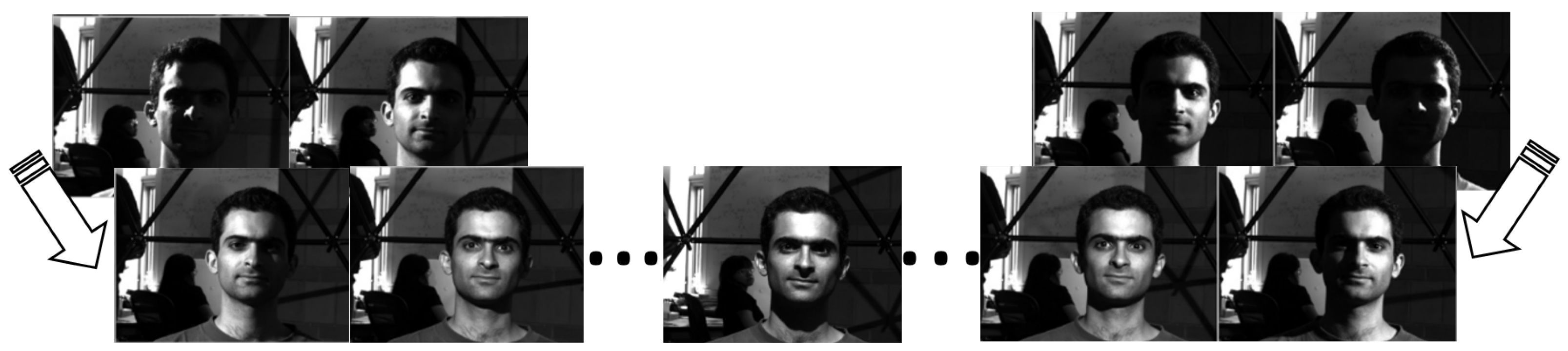
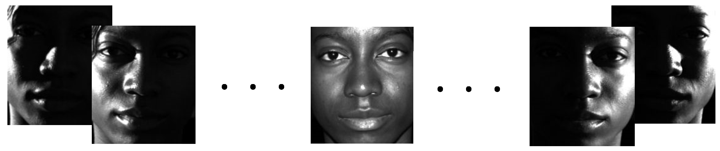
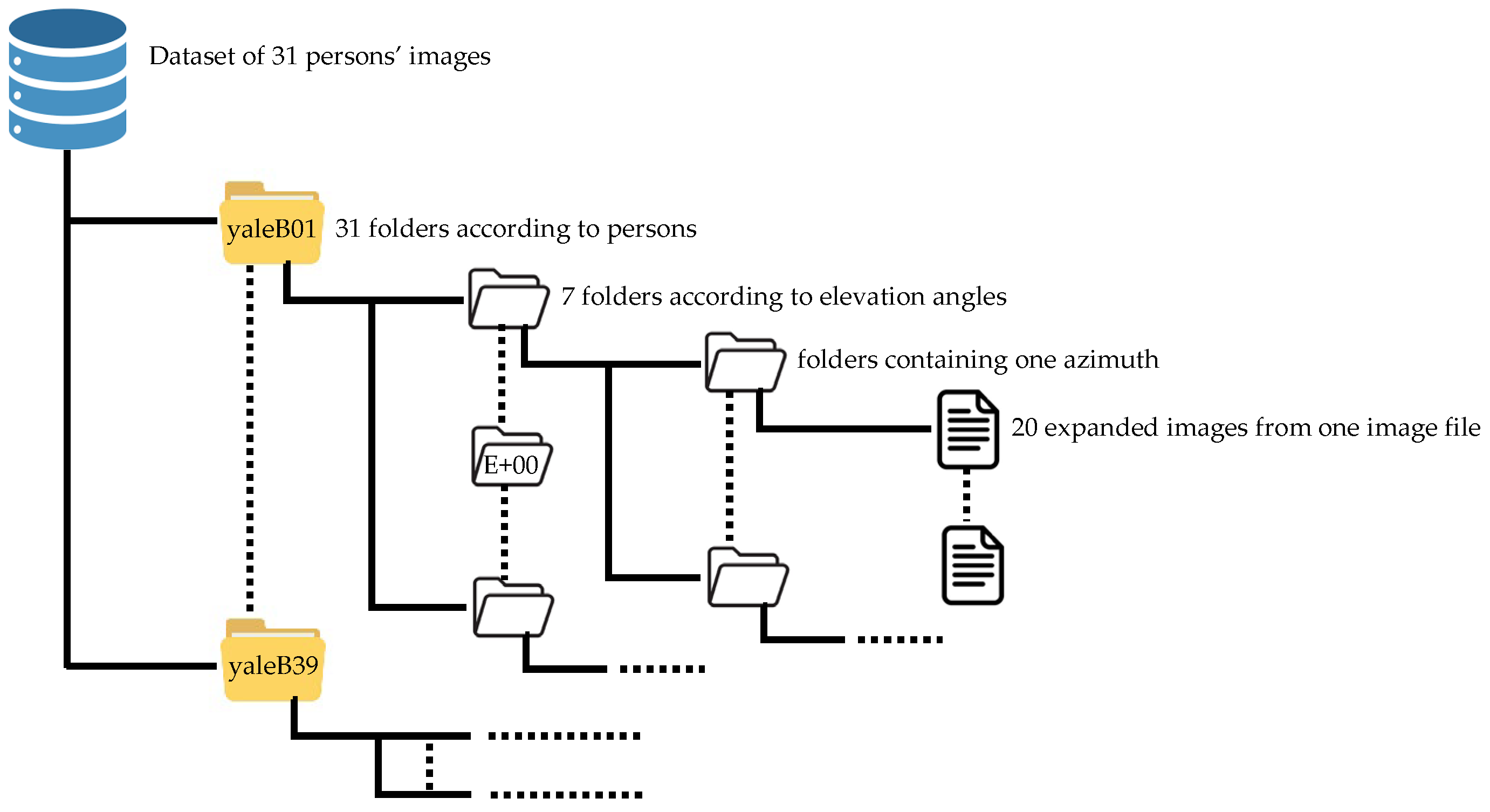
2.1. Data Set

The Extended Yale Face Database B data set [29] is a gray-scale face image data set. Two data sets are provided:
1. Figure 2 is the original image with an azimuth angle of +130° to −130°, the size is 640 × 480 pixels, and there are 28 people in files and 16,128 images in total. Each person has 9 poses, 64 images of environmental lighting changes, and a total of 576 images. The 9 postures include the following: posture 0 is the front posture; postures 1, 2, 3, 4, and 5 are about 12° from the camera’s optical axis (distance from posture 0); and postures 6, 7, and 8 are about 24° [30].
2. Figure 3 shows face images with an azimuth angle of +130° to −130°, all manually aligned, cropped, and adjusted to 168 × 192 pixels. There are 38 people in total and a total of 2432 images. There is only 1 posture for each person, 64 images of environmental lighting changes, and a total of 64 personal images. In this study, we used these face images for face recognition [31].
The 64 kinds of ambient lighting are composed of different azimuth and elevation angles. The azimuth angles range from +130° to −130°. The elevation angles range from +090° to −040°. A positive azimuth angle indicates that the light source is on the right side of the object, while a negative azimuth angle indicates that the light source is on the left side of the object. A positive elevation angle means above the horizon, and a negative elevation angle below the horizon.

2.2. Google Colaboratory

Google’s Colaboratory (Colab) provides an interactive environment that allows people to write and execute Python programs and Linux commands on a browser and use TPU and GPU at no cost. Therefore, Colab is suitable for training the small neural network model. In addition, Colab is not a static web page but a "Colab notebook”. One can edit the code, add comments, pictures, HTML, LaTeX, and other formats, execute the code in sections, and save the current output results on Colab.

2.3. Python Libraries
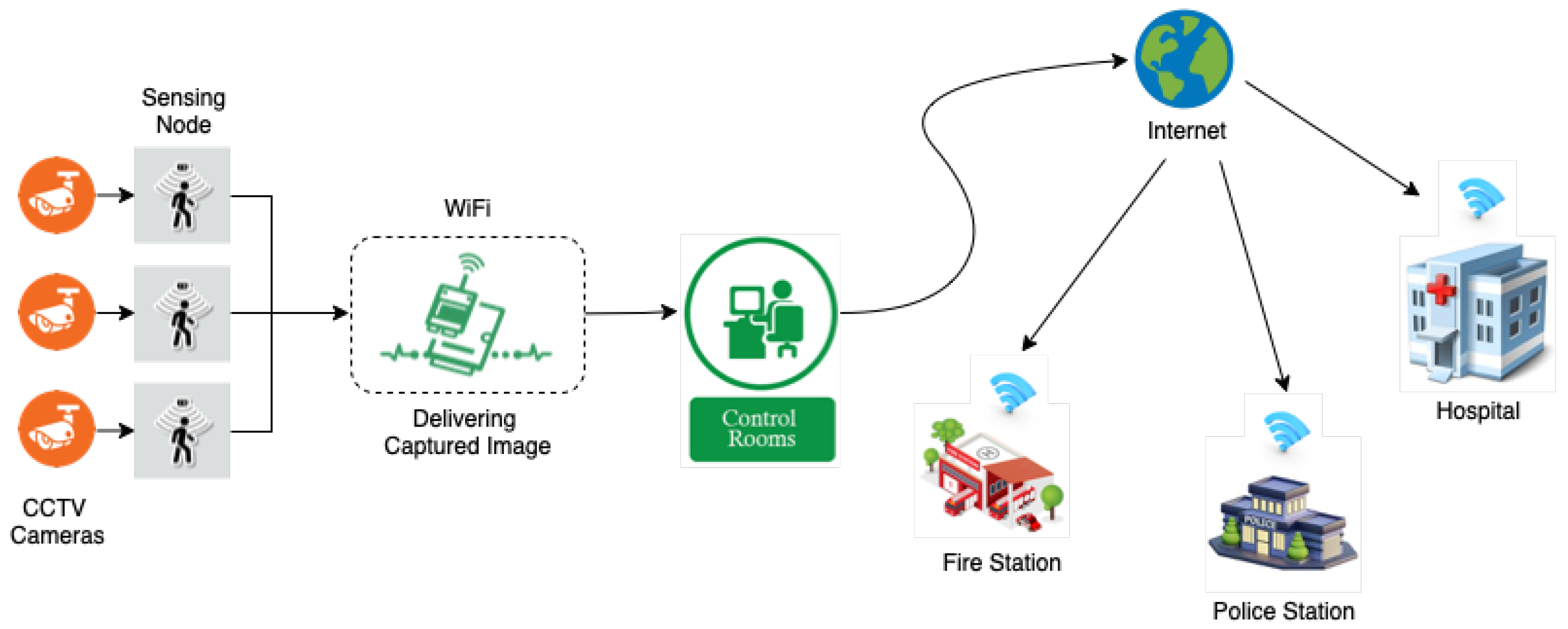
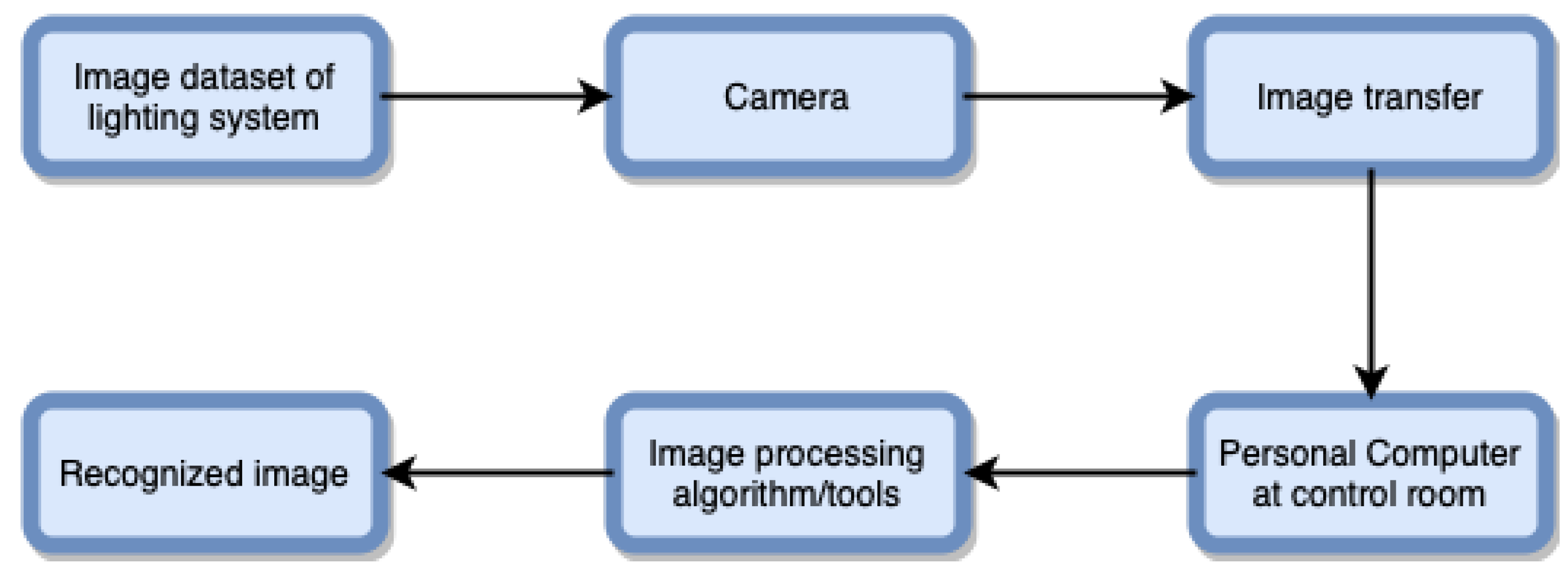
The face recognition algorithms and packages used in this study are all written in the Python 3 programming language. The main libraries used are shown in Table 1.
The opencv and imutils packages were mainly used for image processing. The opencv functions included building LBPH face recognition models, reading images and caffe, executing TensorFlow and other deep learning models, image pre-processing, capturing images from cameras, and displaying images. The imutils program was used in conjunction with opencv to calculate the number of image frames, resize the image, and maintain the image’s aspect ratio. The keras library was used for data enhancement. It randomly performed operations such as horizontal translation, vertical translation, zooming, and horizontal flipping on the image to generate many similar images, increasing the number of images for training. The numpy library was used for one-dimensional array and matrix operations (images). The sklearn library was used to split the training set and test set, do label coding, execute model performance evaluation, and implement OpenFace’s classifier—SVM. The pickle library was used to save the state of the object as a binary file for use in the next import program, in training, and in test data, and to train an SVM classifier and label encoder (LabelEncoder). The sqlite3 library was used to store image paths, prediction results, and statistical results of training and testing. The matplotlib library was used to visualize the statistical results.

2.4. Data Transfer

Wi-Fi networks are currently the most popular type of signal exchange for local area networks and internet access [32]. The fully advanced wireless technology offers the possibility to take advantage of Wi-Fi-based sensor networks as wireless transmitting has its greatest influence on outdoor areas [33]. Additionally, 100 transmitters and receivers can be supported by each Wi-Fi communication unit [34]. In the context of Wi-Fi-based WSNs’ behavior, an heuristic strategy known as ADVISES (AutomateD Verification of wSn with Event calculuS) provides a mechanism to understand when sequences of events occur, to drive design decisions, to add or drop nodes, and to investigate the expected minimum channel quality required for a WSN to work [35].
Sending high-resolution multi-spectral pictures between a camera and an application can be particularly difficult, especially if transfer durations must be reduced or equal to image frame timings to avoid congestion in image data transmission [36]. Figure 4 describes a method of delivering pictures to clients over various transceiver connections that matches diverse transceiver technologies such as Ethernet, ESATA/SAS, and PCI Express. Standard data are transmitted over the transceiver lines from the source, without any modifications in format or image processing.
After receiving and transferring the image to a personal computer (PC) in the control room, the suggested approaches, LBPH and OpenFace, were utilized to validate the images. In the next step, the image data set was evaluated, and the algorithms successfully recognized the image’s features before transmitting it to automatic detection applications.
To guarantee the most precise image data transfer from the sensing field into crucial applications, the WSN’s Quality of Service (QoS) must be maintained for as long as possible by paying attention to coverage, topology, scheduling mechanism, deployment strategy, security, density, packet transfer distance, memory, data aggregation, battery, etc. [37], all of which are summarized in Table 2. This strategy has a substantial long-term impact on network effectiveness.

3. Experiment Methods

3.1. LBPH: Face Recognition Algorithm

LBPH is a method that can extract the texture features of the image through a local binary pattern (LBP) and conduct statistics through a series of histograms. Finally, after calculating the face distance using the Euclidean distance, LBPH outputs the classification result.

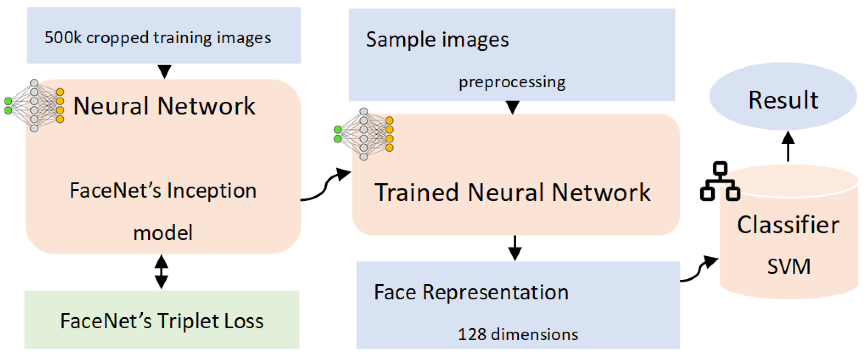
3.2. OpenFace: Face Recognition Algorithm

The model used in the research was the OpenFace model nn4.small2.v1, and the network structure is shown in Figure 5. The accuracy of this model was 0.9292 ± 0.0134 [49], which was based on the Labeled Faces in the Wild (LFW) data set [50] as a benchmark. The Area Under Curve (AUC) was close to 1, which shows the high accuracy of the model’s prediction. The AUC of the nn4.small2.v1 model was 0.973.

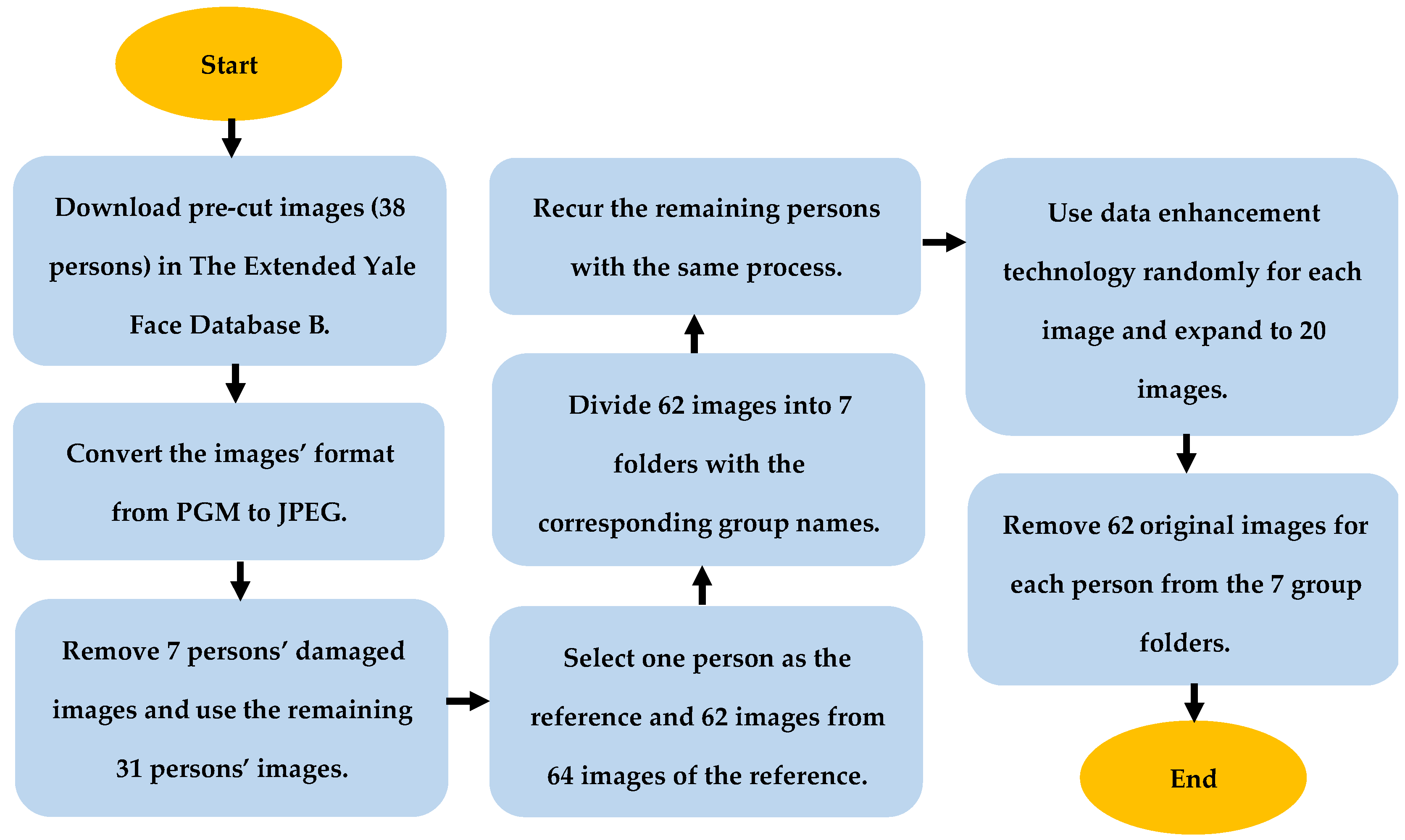
3.3. Data Pre-Processing

First, we downloaded 38 people’s pre-cut face images in The Extended Yale Face Database B data set from the website and converted the images’ format from PGM to JPEG for better image management. Among the downloaded images, 7 people’s images were partially damaged and removed, and the remaining 31 people’s images were applied in the research.
Next, we selected 1 of 31 people as the reference and 62 images (including duplicate images) from 64 images as the reference. We then divided these images into 7 groups according to the elevation angles (refer to Table 3), created 7 folders with the group name, and put the images into the corresponding folder. We used the procedure to repeat the same process with the remaining 30 people exactly as followed for that of the reference person, as shown in Figure 6. We used data enhancement technology for each image in each group by randomly panning, zooming, and flipping the images horizontally. Each image was expanded to 20 images and was stored in a folder with the same name as the image itself.
Finally, the 62 original images for each person were removed from the 7 group folders. Refer to Figure 7 for the complete process above.
To briefly explain the rules of naming image names, the image name of yaleB01_P00A+000E+00 in Table 2 is used as an example: yaleB01 represents a person’s name, and the three capital English letters P, A, and E represent Posture, Azimuth, and Elevation, respectively. In this study, only one posture existed for every person, and thus Posture is recorded as P00.

3.4. Data Set Split

As shown in Table 4, all the images after data enhancement were divided into two parts: 80% of the images were the training set, and 20% of the images were the test set. However, the division was different from the traditional splitting method. Traditionally, 80% of everyone’s images are added up to form the training set, and 20% of everyone’s images are added up to form the test set.
In this paper, the new splitting method was to read the 20 images after each data enhancement in each group of personal images and split each group into a training set and a test set. Thus, in each enhancement image group, there were 16 training set images and 4 test set images. The number of sheets in the training set and test set for each personal image was calculated according to Formulas (1) and (2).
Training set: 62 sheets × (20 sheets × 0.8) = 992 sheets
Test set: 62 sheets × (20 sheets × 0.2) = 248 sheets
Multiplying Formulas (1) and (2) by 31 (people) was the number of sheets in the training set and test set, as shown in Table 3. The reason for splitting immediately was that the prediction accuracy of each image needed to be counted later. If the traditional data splitting method were used, the data splitting would have been uneven, and the subsequent statistics would have lost accuracy.

3.5. LBPH Model Training

First, we divided the image list of the data set (all image paths) into a training set and a test set and stored them in the Python list. Next, we extracted the person’s name from the path of each image as a label and saved it in the Python list. Finally, we serialized the image path and label of each test set into a binary file and saved it to the hard disk.
We read the images of the training set, converted them to gray-scale images, and added them to the Python list. Through the label encoder, we encoded all tags into corresponding numbers, which represented the same person. Next, all gray-scale images and encoded labels were sent into the LBPH model for training. After the model was trained, we saved the LBPH model as a yaml format file and saved the label encoder as a binary file through serialization.

3.6. OpenFace Model Training

First, we divided the image list of the data set (all image paths) into a training set and a test set, extracted the names of people from each image path as labels, and stored them in the Python list. We then stored the image paths and tags of the training set and the test set into the SQLite database.
We read the image of the training set and set the image size to a width of 600 pixels, and the height was automatically adjusted with the width to maintain the aspect ratio. We used opencv’s blobFromImage function to perform channel exchange, feature normalization, and image size adjustment to 96 × 96 pixels. We sent the image to the OpenFace pre-trained neural network nn4.small2.v1 model for inference and then output a 128-dimensional feature vector.
We used numpy’s flatten function to flatten the 128-dimensional vector into a one-dimensional array and added the array to the Python list. After we read the images of the test set and skipped a flattened procedure, the images of the test set were processed in the same way as the training set and finally stored in the Python list.
While the labels were encoded in the same way as in LBPH, the 128-dimensional feature vector of the training set and the encoded labels were sent into the SVM classifier for training. After training, the SVM classifier, the label encoder, the 128-dimensional feature vector of the test set, and the names of the test set were individually stored as binary files through serialization.

3.7. LBPH Prediction Image

We loaded the trained LBPH model and label encoder from the hard disk and retrieved the image paths and tags of all test sets from the binary file. From the image path of each test set, we extracted the person’s name, group name, and file name. We read all the images, converted them into gray-scale images, and saved them into the Python list. In the label part, the name of the person was label-encoded and converted into the corresponding number. We sent all gray-scale images into the LBPH model for prediction. After the prediction was completed, we saved the group name, file name, test label, prediction label, and prediction distance into the Python list. We then used the Python dictionary to store the list with the name of the person as the key and the data as the value, and we saved the dictionary as a binary file through serialization. Through deserialization, the binary dictionary file was read, and the person’s name, group name, file name, test label, predicted label, and predicted distance in the list were extracted out from the dictionary by using the name of the person as the key. We then compared the test tags with the predicted tags one by one and recorded the identification results. At the end, the serial number, group name, file name, test label, predicted label, predicted distance, and identification result were stored in the SQLite database together.

3.8. OpenFace Prediction Image

We read the trained SVM classifier, label encoder, test set images, and labels from memory through deserialization. We encoded the label through the label encoder and converted it into a corresponding number. We used the SVM classifier to predict each test set image and store the prediction results and probabilities. We pulled the image path of all test sets from the SQLite database and extracted the file name and group name from it. We compared the label of the test set with the predicted result and recorded the identification result. Finally, the serial number, person name, group name, file name, coded test set label, predicted label, predicted probability, and identification result were stored in the SQLite database.

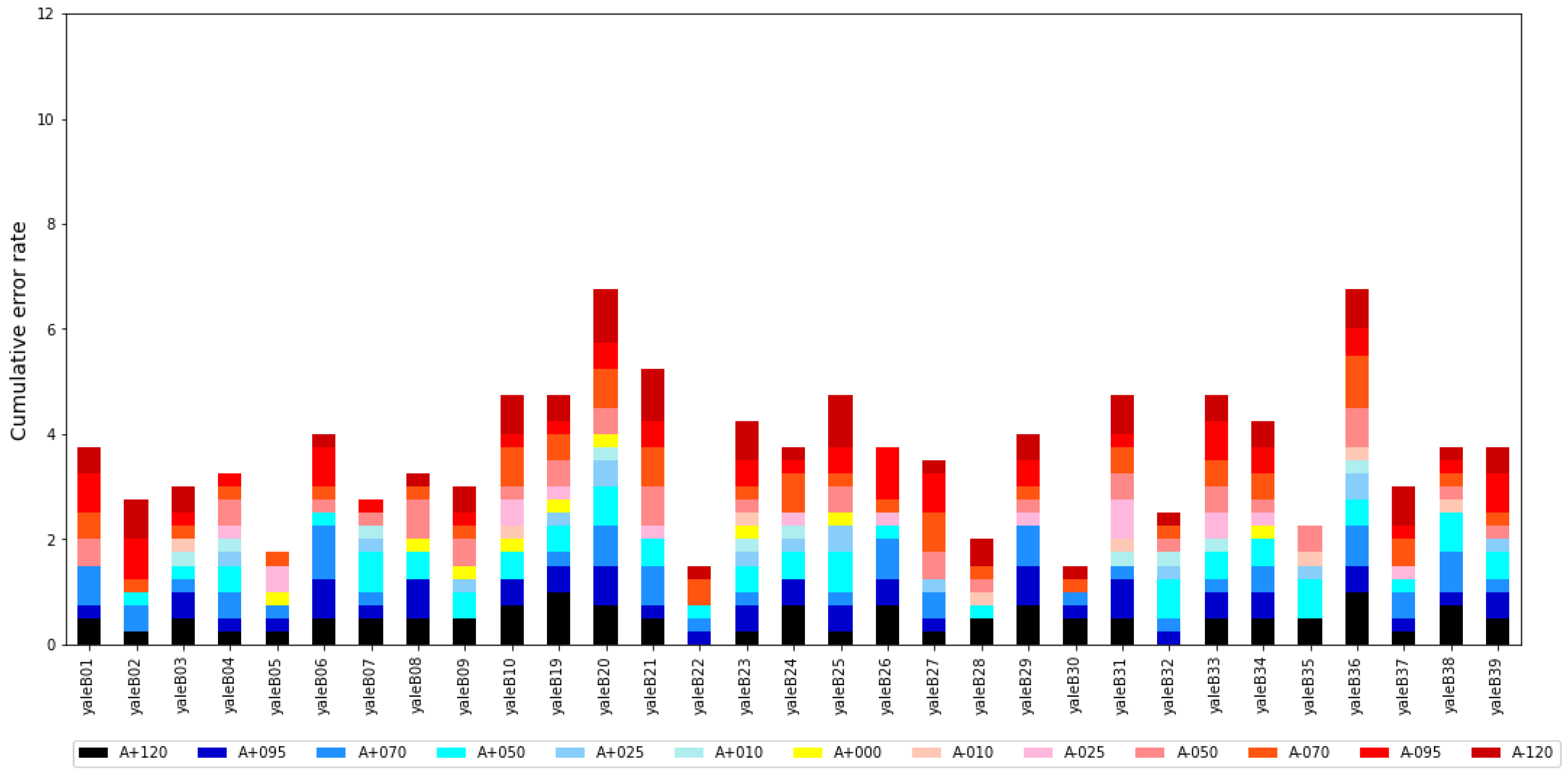
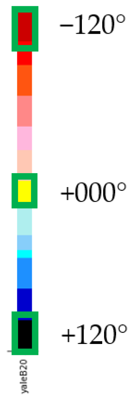
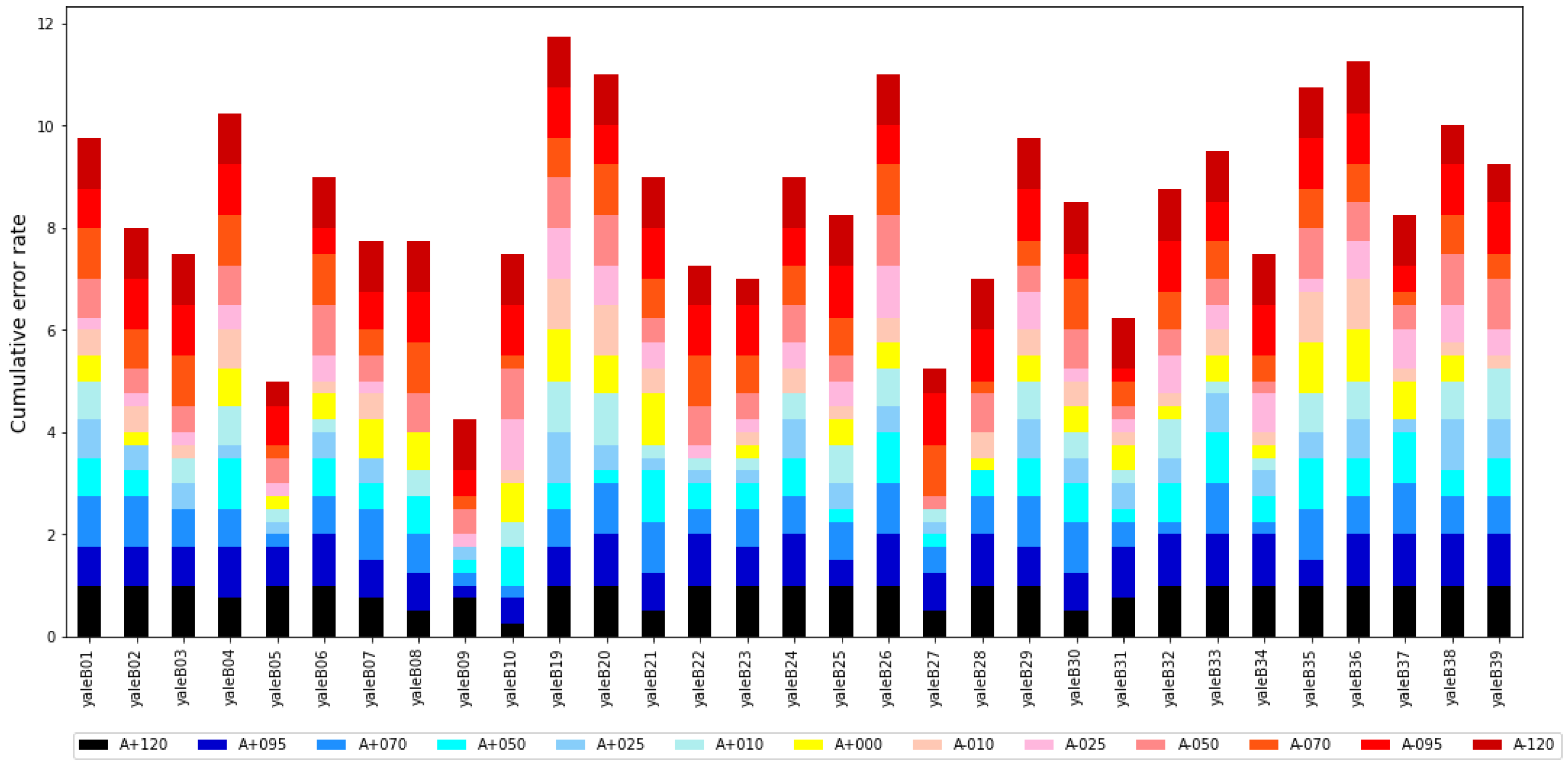
3.9. Statistics and Visualization

We obtained the prediction results from the SQLite database of LBPH and OpenFace. We counted the number of correct and incorrect predictions for each image of each group and saved the number, person name, group name, file name, status, and quantity into the SQLite database.
For the visualization part, we selected the A+120--120E+00 grouping, shown in Figure 8, for more detailed statistics. This group consisted of 13 photos, where A+120--120 meant the range was from +120° to −120° in azimuth and E+00 meant elevation was 0°. The reason for choosing this group was that the range of azimuth angles in this group was widely distributed, and E+00 made illumination even in the longitudinal plane. With A+000 as the center, the lighting effect was symmetrical on the face and was easier to observe, at which the azimuth will cause the accuracy to rise or fall sharply.

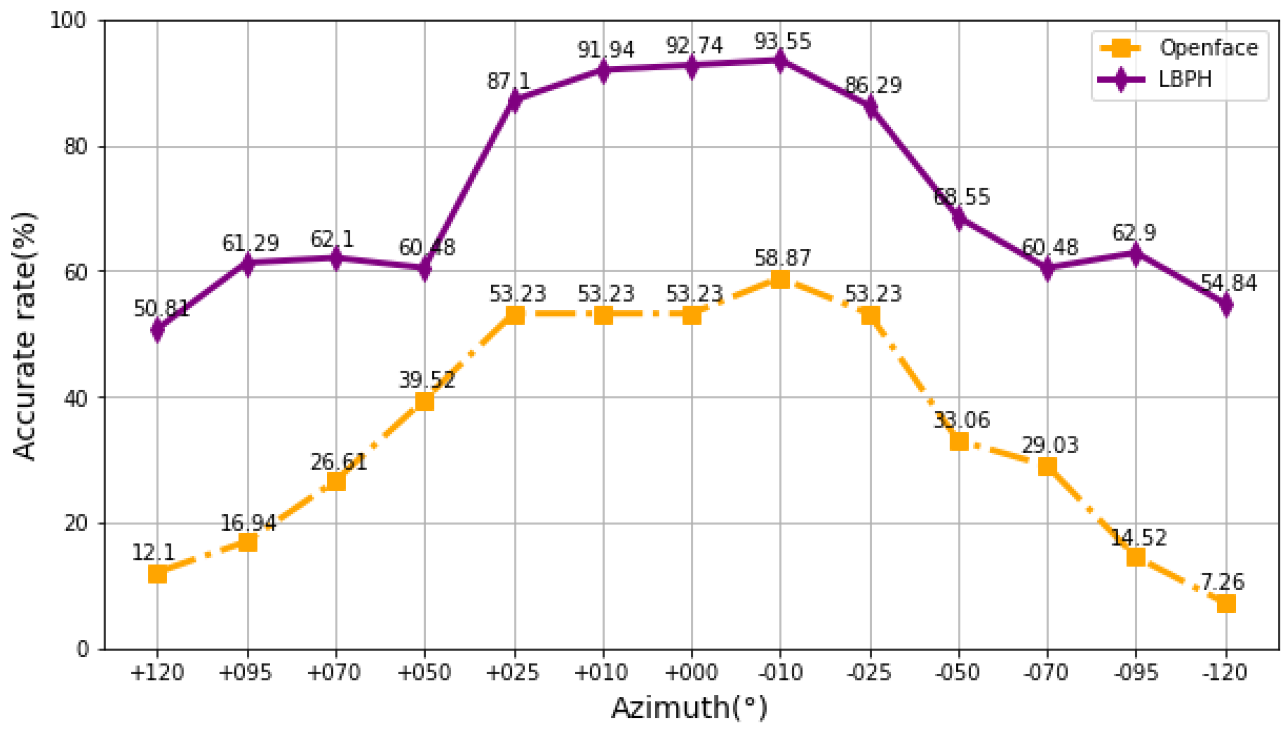
4. Experimental Results

Figure 9 is a stacking diagram of LBPH’s A+120--120E+00 grouping error rate comparison of different ambient light levels. Figure 10 illustrates the stacking method of Figure 9. The bottom of the stacked image is the azimuth +120°, the center white block is the azimuth +000°, and the top is the azimuth −120°. The recognition error rate is lower closer to the center white block, and higher otherwise. Therefore, the recognition error rates of the uppermost and the lowermost blocks are the highest, and the recognition error rate decreases as the azimuth angle approaches +000°.
Figure 11 is a stacking diagram of OpenFace’s A+120--120E+00 grouping error rate comparison of different ambient light levels. The recognition error rates of the uppermost and the lowermost blocks are the highest, and they decrease as the azimuth angle approaches +000°. Overall, OpenFace’s recognition error rate was about 20% to 49% higher than LBPH’s in A+120--120E+00 grouped images.
Accurate   rate = 1 31 ( (   Number   of   correctly   identified   sheets ÷ 4 ) × 100 % ) ÷ 31
Figure 12 shows the average ambient lighting accuracy rates of 31 people grouped by A+120--120E+00. Formula (3) is the calculation formula for the average recognition accuracy rates of each azimuth angle in Figure 12.
First, we calculated the ratio of the number of correct predictions to the total number of predictions and then converted the ratio into a percentage. Finally, we added up all the percentages and divided by 31 people to get the average.
For the picture with A+000° as the center line, the recognition accuracy rate was almost symmetrical. There was not much difference between the light source on the left or the right. The closer the recognized azimuth angle was to azimuth +000°, the higher the recognition accuracy rate; the farther away the azimuth angle +000°, the lower the recognition accuracy rate. Overall, the recognition accuracy rate of LBPH under changes in environmental lighting was far better than that of OpenFace. Therefore, LBPH is more suitable for applications in environments with light changes. From Figure 12, whether LBPH or OpenFace was used at the azimuth angle of −010°, the recognition accuracy rate was the highest. LBPH was 34.68% more accurate than OpenFace at the azimuth angles of −010°. LBPH was 38.71% more accurate than OpenFace at the azimuth angles of +120°.
Error   rate =     1 31   ( (   Number   of   sheets   with   identification   errors ÷ 4 ) × 100 % ) ÷ 31
Figure 13 shows the average ambient light error rate of 31 people grouped by A+120--120E+00, and Formula (4) is the calculation formula for the average identification error rate of each azimuth angle shown in Figure 13. First, we calculated the ratio of the number of prediction errors to the total number of predictions and converted it into a percentage. Finally, we added up all percentages and divided by 31 people to get the average.
With A+000° as the center line, the recognition error rate was almost symmetrical. Overall, the recognition error rate of LBPH was much lower than that of OpenFace. When both azimuth angles were in the range of +25° to −25°, the recognition error rate was relatively low. When both azimuth angles were in the range of +50° to +120° and −50° to −120°, the recognition error rate was relatively high. For LBPH, when the azimuth angle was +50° to +25°, the identification error rate was reduced by 26.62%; when the azimuth angle was −50° to −25°, the identification error rate was reduced by 17.74%. For OpenFace, when the azimuth angle was +50° to +25°, the recognition error rate dropped by 13.71%; when the azimuth angle was -50° to −25°, the recognition error rate dropped by 20.17%. From the azimuth angle of +50° to +25° and −50° to −25°, we found that the recognition error rate was significantly reduced. This means that the change of the azimuth angle reduces the shadow on the face, and the contours of the facial features are clearer, reducing the error rate of face recognition.

5. Discussion

The benefits and drawbacks of both LBPH and OpenFace were published in previous studies [27]. In general, OpenFace has consistently higher accuracy than that of LBPH in adding more samples, although increasing the number of samples makes overall accuracy drop. OpenFace’s SVM has faster training time than that of LBPH, no matter how many samples are included. In times of prediction per image, OpenFace increases slightly more than LBPH does, but it does not increase further while increasing the sample numbers. With sample sizes larger than 50, the prediction time per image of LBPH exceeds that of OpenFace executed on a GPU.
The circumstances of images have great influence on the accuracy of these two methods [51]. Image noises affect LBPH more than OpenFace. Under various camera resolutions, OpenFace shows more robustly than LBPH. However, in different lighting conditions, LPBH operates better than OpenFace.
According to the least required amount of training data to achieve a good result, OpenFace requires fewer than 20 images per person to achieve 95% accuracy, while LBPH requires far more to achieve similar results. A main advantage of OpenFace is its design for real-time identification and that it can be easily worked on mobile devices. One can use very little data to train an OpenFace model to achieve high accuracy.
LBPH is superior to OpenFace in that it works better in unevenly lighting circumstances. LBPH is suitable in systems with inconsistent illumination, such as payment systems. LBPH is less affected by different lighting because of its calculation of each pixel’s binary number according to neighborhood, which can reduce interference of nearby illumination. Throughout the procedure, LBPH can reflect the local characteristics of each pixel.
The previous studies did not analyze in detail the impact of various lightings on face recognition, nor did they conduct thorough research on the two methods at different illumination angles. We confirmed that in terms of different lighting angles, LBPH is more consistently accurate than OpenFace. LBPH has an accuracy of close to or more than 90%, especially while the lighting angle is within + or - 25 degrees in the horizontal plane.

6. Conclusions and Future Work

From the results, LBPH is more suitable than OpenFace in recognition applications with ambient lighting changes. When the light source is kept larger than the azimuth angle of +25° or less than −25° and the elevation angle +000°, the shadows on the face will increase, and the recognition accuracy will be lower; if not, the result will be the reverse. According to the results of face recognition with changes in ambient light, compared with that of the OpenFace recognition model, LBPH has superior performance in classification and recognition.
Therefore, for image recognition (such as face recognition) that requires more detailed output for line texture features but is affected by ambient light, LBPH has a greater level of recognition accuracy for its object recognition or classification results than that of OpenFace. Furthermore, the previously made important image collection can be employed in the subsequent data transfer process.
In addition, most facial images are captured in natural settings. As a result, the contents of the picture can be very complicated, and the lightening state can be very diverse. The other major problems of images from cameras are distortion, noise, and different resolutions of lens systems. Applying the appropriate methods will improve the system and make it more robust and efficient so that it can be implemented in realistic settings.
Since a trained LBPH algorithm is very robust to changes in ambient light, it can be deployed on a Raspberry Pi or other edge computing processors to be implemented in access control systems with ambient lighting changes or related fields of applications, such as facial payment systems.

Author Contributions

Conceptualization, Y.-C.C. and Y.-S.L.; data curation, H.-Y.S. and Y.-C.S.; methodology, Y.-C.C., Y.-S.L. and M.S.; software, H.-Y.S. and Y.-C.S.; formal analysis, Y.-C.C. and Y.-S.L.; resources, M.S. and Y.-C.S.; writing—original draft preparation, Y.-S.L. and Y.-C.S.; writing—review and editing, M.S. and H.-Y.S.; supervision, Y.-C.C., H.-Y.S. and M.S. All authors have read and agreed to the published version of the manuscript.

Funding

This research received no external funding.

Institutional Review Board Statement

Not applicable.

Informed Consent Statement

Not applicable.

Data Availability Statement

Simulated data can be provided upon request.

Conflicts of Interest

The authors declare no conflict of interest.

References

  1. Abd Al Rahman, M.; Mousavi, A. A review and analysis of automatic optical inspection and quality monitoring methods in electronics industry. IEEE Access 2020, 8, 183192–183271. [Google Scholar] [CrossRef]
  2. Adini, Y.; Moses, Y.; Ullman, S. Face recognition: The problem of compensating for changes in illumination direction. IEEE Trans. Pattern Anal. Mach. Intell. 1997, 19, 721–732. [Google Scholar] [CrossRef] [Green Version]
  3. Alshamsi, H.; Meng, H.; Li, M. Real time facial expression recognition app development on mobile phones. In Proceedings of the 2016 12th International Conference on Natural Computation, Fuzzy Systems and Knowledge Discovery (ICNC-FSKD), Changsha, China, 3–15 August 2016; pp. 1750–1755. [Google Scholar]
  4. Huang, T.; Xiong, Z.; Zhang, Z. Face Recognition Applications. In Handbook of Face Recognition; Springer: Berlin/Heidelberg, Germany, 2005; pp. 371–390. [Google Scholar]
  5. Wheeler, F.W.; Weiss, R.L.; Tu, P.H. Face recognition at a distance system for surveillance applications. In Proceedings of the 2010 Fourth IEEE International Conference on Biometrics: Theory, Applications and Systems (BTAS), Washington, DC, USA, 27–29 September 2010; pp. 1–8. [Google Scholar]
  6. Pahuja, N. Smart Cities and Infrastructure Standardization Requirements. In Solving Urban Infrastructure Problems Using Smart City Technologies; Elsevier: Amsterdam, The Netherlands, 2021; pp. 331–357. [Google Scholar]
  7. Ijaz Ul Haq, K.M.; Sajjad, M.; Lee, M.Y.; Han, D.; Baik, S.W. A Study of Data Dissemination in CCTV Surveillance Systems. Image 2016, 75, 14867–14893. [Google Scholar]
  8. Mittal, A.; Davis, L.S. Visibility Analysis and Sensor Planning in Dynamic Environments. In European Conference on Computer Vision; Springer: Berlin/Heidelberg, Germany, 2004; pp. 175–189. [Google Scholar]
  9. Meesookho, C.; Narayanan, S.; Raghavendra, C. Collaborative classification applications in sensor networks. In Proceedings of the Sensor Array and Multichannel Signal Processing Workshop Proceedings, Trondheim, Norway, 20–23 June 2002; pp. 370–374. [Google Scholar]
  10. Mainwaring, A.; Culler, D.; Polastre, J.; Szewczyk, R.; Anderson, J. Wireless sensor networks for habitat monitoring. In Proceedings of the 1st ACM International Workshop on WIRELESS Sensor Networks and Applications, Atlanta, GA, USA, 28 September 2002; pp. 88–97. [Google Scholar]
  11. Williams, A.; Ganesan, D.; Hanson, A. Aging in place: Fall detection and localization in a distributed smart camera network. In Proceedings of the 15th ACM International Conference on Multimedia, New York, NY, USA, 24–29 September 2007; pp. 892–901. [Google Scholar]
  12. Zhu, X.; Ding, B.; Li, W.; Gu, L.; Yang, Y. On development of security monitoring system via wireless sensing network. EURASIP J. Wirel. Commun. Netw. 2018, 2018, 221. [Google Scholar] [CrossRef] [Green Version]
  13. Zhao, W.; Chellappa, R.; Phillips, P.J.; Rosenfeld, A. Face recognition: A literature survey. ACM Comput. Surv. (CSUR) 2003, 35, 399–458. [Google Scholar] [CrossRef]
  14. Zhang, J.; Yan, Y.; Lades, M. Face recognition: Eigenface, elastic matching, and neural nets. Proc. IEEE 1997, 85, 1423–1435. [Google Scholar] [CrossRef]
  15. Belhumeur, P.N.; Hespanha, J.P.; Kriegman, D.J. Eigenfaces vs. fisherfaces: Recognition using class specific linear projection. IEEE Trans. Pattern Anal. Mach. Intell. 1997, 19, 711–720. [Google Scholar] [CrossRef] [Green Version]
  16. Ahonen, T.; Hadid, A.; Pietikäinen, M. Face Recognition with Local Binary Patterns. In European Conference on Computer Vision; Springer: Berlin/Heidelberg, Germany, 2004; pp. 469–481. [Google Scholar]
  17. Liu, W.; Wang, Z.; Liu, X.; Zeng, N.; Liu, Y.; Alsaadi, F.E. A survey of deep neural network architectures and their applications. Neurocomputing 2017, 234, 11–26. [Google Scholar] [CrossRef]
  18. Lawrence, S.; Giles, C.L.; Tsoi, A.C.; Back, A.D. Face recognition: A convolutional neural-network approach. IEEE Trans. Neural Netw. 1997, 8, 98–113. [Google Scholar] [CrossRef] [Green Version]
  19. Tan, X.; Triggs, B. Enhanced local texture feature sets for face recognition under difficult lighting conditions. IEEE Trans. Image Process. 2010, 19, 1635–1650. [Google Scholar]
  20. Howse, J. Training Detectors and Recognizers in Python and OpenCVn. In Proceedings of the 2014 IEEE International Symposium on Mixed and Augmented Reality (ISMAR), Munich, Germany, 10–12 September 2014; IEEE Computer Society: Washington, DC, USA, 2014; pp. 1–2. [Google Scholar]
  21. Shoba, V.B.T.; Sam, I.S. Face recognition using LBPH descriptor and convolution neural network. In Proceedings of the 2018 Second International Conference on Intelligent Computing and Control Systems (ICICCS), Madurai, India, 14–15 June 2018; pp. 1439–1444. [Google Scholar]
  22. Mondal, I.; Chatterjee, S. Secure and hassle-free EVM through deep learning based face recognition. In Proceedings of the 2019 International Conference on Machine Learning, Big Data, Cloud and Parallel Computing (COMITCon), Faridabad, India, 14–16 February 2019; pp. 109–113. [Google Scholar]
  23. Zhuang, L.; Guan, Y. Deep learning for face recognition under complex illumination conditions based on log-gabor and LBP. In Proceedings of the 2019 IEEE 3rd Information Technology, Networking, Electronic and Automation Control Conference (ITNEC), Chengdu, China, 15–17 May 2019; pp. 1926–1930. [Google Scholar]
  24. Soo, S. Object detection using Haar-cascade Classifier. Inst. Comput. Sci. Univ. Tartu 2014, 2, 1–12. [Google Scholar]
  25. Dalal, N.; Triggs, B. Histograms of oriented gradients for human detection. In Proceedings of the 2005 IEEE Computer Society Conference on Computer Vision and Pattern Recognition (CVPR’05), San Diego, CA, USA, 20–26 June 2005; Volume 1, pp. 886–893. [Google Scholar]
  26. Schroff, F.; Kalenichenko, D.; Philbin, J. Facenet: A unified embedding for face recognition and clustering. In Proceedings of the IEEE Conference on Computer Vision and Pattern Recognition, Boston, MA, USA, 7–12 June 2015; pp. 815–823. [Google Scholar]
  27. Amos, B.; Ludwiczuk, B.; Satyanarayanan, M. Openface: A general-purpose face recognition library with mobile applications. CMU Sch. Comput. Sci. 2016, 6, 20. [Google Scholar]
  28. Baltrusaitis, T.; Zadeh, A.; Lim, Y.C.; Morency, L.-P. Openface 2.0: Facial behavior analysis toolkit. In Proceedings of the 2018 13th IEEE International Conference on Automatic Face & Gesture Recognition (FG 2018), Xi’an, China, 15–18 May 2018; pp. 59–66. [Google Scholar]
  29. Diego, U.o.C.S. The Extended Yale Face Database B. Available online: http://vision.ucsd.edu/~leekc/ExtYaleDatabase/ExtYaleB.html (accessed on 30 September 2020).
  30. Georghiades, A.S.; Belhumeur, P.N.; Kriegman, D.J. From few to many: Illumination cone models for face recognition under variable lighting and pose. IEEE Trans. Pattern Anal. Mach. Intell. 2001, 23, 643–660. [Google Scholar] [CrossRef] [Green Version]
  31. Lee, K.-C.; Ho, J.; Kriegman, D.J. Acquiring linear subspaces for face recognition under variable lighting. IEEE Trans. Pattern Anal. Mach. Intell. 2005, 27, 684–698. [Google Scholar] [PubMed]
  32. Zhou, Z.; Wu, C.; Yang, Z.; Liu, Y. Sensorless sensing with WiFi. Tsinghua Sci. Technol. 2015, 20, 1–6. [Google Scholar] [CrossRef]
  33. Kirkpatrick, K. World Without Wires; ACM: New York, NY, USA, 2014. [Google Scholar]
  34. Yu, Y.; Han, F.; Bao, Y.; Ou, J. A study on data loss compensation of WiFi-based wireless sensor networks for structural health monitoring. IEEE Sens. J. 2015, 16, 3811–3818. [Google Scholar] [CrossRef]
  35. Testa, A.; Cinque, M.; Coronato, A.; De Pietro, G.; Augusto, J.C. Heuristic strategies for assessing wireless sensor network resiliency: An event-based formal approach. J. Heuristics 2015, 21, 145–175. [Google Scholar] [CrossRef] [Green Version]
  36. Zanjani, P.N.; Bahadori, M.; Hashemi, M. Monitoring and remote sensing of the street lighting system using computer vision and image processing techniques for the purpose of mechanized blackouts (development phase). In Proceedings of the IET Digital Library of 22nd International Conference and Exhibition on Electricity Distribution (CIRED 2013), 10–13 June 2013; Stockholm, Sweden. [Google Scholar]
  37. Farhat, A.; Guyeux, C.; Makhoul, A.; Jaber, A.; Tawil, R.; Hijazi, A. Impacts of wireless sensor networks strategies and topologies on prognostics and health management. J. Intell. Manuf. 2019, 30, 2129–2155. [Google Scholar] [CrossRef] [Green Version]
  38. Younis, M.; Senturk, I.F.; Akkaya, K.; Lee, S.; Senel, F. Topology management techniques for tolerating node failures in wireless sensor networks: A survey. Comput. Netw. 2014, 58, 254–283. [Google Scholar] [CrossRef]
  39. Li, M.; Li, Z.; Vasilakos, A.V. A survey on topology control in wireless sensor networks: Taxonomy, comparative study, and open issues. Proc. IEEE 2013, 101, 2538–2557. [Google Scholar] [CrossRef]
  40. Gupta, N.; Kumar, N.; Jain, S. Coverage problem in wireless sensor networks: A survey. In Proceedings of the 2016 International Conference on Signal Processing, Communication, Power and Embedded System (SCOPES), Odisha, India, 3–5 October 2016; pp. 1742–1749. [Google Scholar]
  41. Liang, D.; Shen, H.; Chen, L. Maximum target coverage problem in mobile wireless sensor networks. Sensors 2020, 21, 184. [Google Scholar] [CrossRef] [PubMed]
  42. Chang, R.-S.; Wang, S.-H. Deployment strategies for wireless sensor networks. In Handbook of Research on Developments and Trends in Wireless Sensor Networks: From Principle to Practice; IGI Global: Hershey, PA, USA, 2010; pp. 20–37. [Google Scholar]
  43. Cheng, H.; Su, Z.; Lloret, J.; Chen, G. Service-oriented node scheduling scheme for wireless sensor networks using Markov random field model. Sensors 2014, 14, 20940–20962. [Google Scholar] [CrossRef] [PubMed] [Green Version]
  44. Chen, H.; Li, X.; Zhao, F. A reinforcement learning-based sleep scheduling algorithm for desired area coverage in solar-powered wireless sensor networks. IEEE Sens. J. 2016, 16, 2763–2774. [Google Scholar] [CrossRef]
  45. Darabkh, K.A.; Odetallah, S.M.; Al-qudah, Z.; Ala’F, K.; Shurman, M.M. Energy-aware and density-based clustering and relaying protocol (EA-DB-CRP) for gathering data in wireless sensor networks. Appl. Soft Comput. 2019, 80, 154–166. [Google Scholar] [CrossRef]
  46. Ahmed, M.H.; Alam, S.W.; Qureshi, N.; Baig, I. Security for WSN based on elliptic curve cryptography. In Proceedings of the International Conference on Computer Networks and Information Technology, Abbottabad, Pakistan, 11–13 July 2011; pp. 75–79. [Google Scholar]
  47. Khan, M.A.; Khan, J.; Sehito, N.; Mahmood, K.; Ali, H.; Bari, I.; Arif, M.; Ghoniem, R.M. An Adaptive Enhanced Technique for Locked Target Detection and Data Transmission over Internet of Healthcare Things. Electronics 2022, 11, 2726. [Google Scholar] [CrossRef]
  48. Ozdemir, S.; Xiao, Y. Secure data aggregation in wireless sensor networks: A comprehensive overview. Comput. Netw. 2009, 53, 2022–2037. [Google Scholar] [CrossRef]
  49. OpenFace. Models and Accuracies. Available online: https://cmusatyalab.github.io/openface/models-and-accuracies/ (accessed on 18 September 2022).
  50. Massachusetts, U.O. Labeled Faces in the Wild. Available online: http://vis-www.cs.umass.edu/lfw/ (accessed on 18 September 2022).
  51. Jacob, M.P. Comparison of popular face detection and recognition techniques. Int. Res. J. Mod. Eng. Technol. Sci. e-ISSN 2021, 3, 2582–5208. [Google Scholar]
Figure 1. Reprinted from Ref. [7]: Framework of data transmission in CCTV system.
Electronics 12 00166 g001
Figure 2. Original image with azimuth angle of +130° to −130°.
Electronics 12 00166 g002
Figure 3. Face image with an azimuth angle of +130° to −130°.
Electronics 12 00166 g003
Figure 4. The process of image recognition from multiple cameras into PC.
Electronics 12 00166 g004
Figure 5. OpenFace nn4.small2 network structure.
Electronics 12 00166 g005
Figure 6. Group directory structure.
Electronics 12 00166 g006
Figure 7. Data set processing flow chart.
Electronics 12 00166 g007
Figure 8. Grouped images of A+120--120E+00.
Electronics 12 00166 g008
Figure 9. Comparison of the error rate of LBPH with different ambient light levels.
Electronics 12 00166 g009
Figure 10. Illustration of stacked graphs of different illumination error rates for a single user.
Electronics 12 00166 g010
Figure 11. Comparison of error rate of OpenFace with different ambient light levels.
Electronics 12 00166 g011
Figure 12. Average ambient lighting accuracy rates of A+120--120E+00 group.
Electronics 12 00166 g012
Figure 13. Average ambient light error rate of A+120--−120E+00 group.
Electronics 12 00166 g013
Table 1. List of python libraries.
Librarypurpose
opencvimage processing, LBPH face recognition
imutilsimage processing (package opencv part of the API)
kerasdata enhancement
numpyarray and matrix operations
sklearnmachine learning
pickleobject serialization and deserialization
sqlite3database operations
matplotlibvisualized graphics presentation
Table 2. Comparison of related work by metrics.
WorkMetricsResult
Topology management techniques for tolerating node failures in wireless sensor networks: A survey [38]TopologyThis research examined network topology management approaches for tolerating node failures in WSNs, categorizing them into two major categories based on reactive and proactive approaches.
A survey on topology control in wireless sensor networks: Taxonomy, comparative study, and open issues [39] Existing topology control strategies were classified into two categories in this study: network connectivity and network coverage. Spikes of existing protocols and techniques were offered for each area, with a focus on barrier coverage, blanket coverage, sweep coverage, power control, and power management.
Coverage problem in wireless sensor networks: A survey [40]CoverageTo obtain significant results, the integration of both coverage and connectivity was required.
Maximum target coverage problem in mobile wireless sensor network [41] The Maximum Target Coverage with Limited Mobile (MTCLM) COLOUR algorithm performed well when the target density was low.
Deployment strategies for wireless sensor networks [42]DeploymentThe deployment affected the efficiency and the effectiveness of sensor networks.
Service-oriented node scheduling scheme for wireless sensor networks using Markov random field model [43]SchedulingA new MRF-based multi-service node scheduling (MMNS) method revealed that the approach efficiently extended network lifetime.
A reinforcement learning-based sleep scheduling (RLSSC) algorithm for desired area coverage in solar-powered wireless sensor networks [44] The results revealed that RLSSC could successfully modify the working mode of nodes in a group by recognizing the environment and striking a balance of energy consumption across nodes to extend the network’s life, while keeping the intended range.
Energy-aware and density-based clustering and relaying protocol (EA-DB-CRP) for gathering data in wireless sensor networks [45]DensityA proposed energy-aware and density-based clustering and routing protocol (EA-DB-CRP) had a significant impact on network lifetime and energy utilization when compared to other relevant studies.
Security for WSN based on elliptic curve cryptography [46]SecurityThe installation of the 160-bit ECC processor on the Xilinx Spartan 3an FPGA met the security requirements of sensor network designed to achieve speed in 32-bit numerical computations.
An Adaptive Enhanced Technique for Locked Target Detection and Data Transmission over Internet of Healthcare Things [47] Color and gray-scale image with varied text sizes, combined with encryption algorithms (AES and RSA), gave superior outcomes in a hybrid security paradigm for data protection diagnostic text.
Secure data aggregation in wireless sensor networks [48]Data aggregationThe study presented a thorough examination of the notion of secure data aggregation in wireless sensor networks, focusing on the relationship between data aggregation and its security needs.
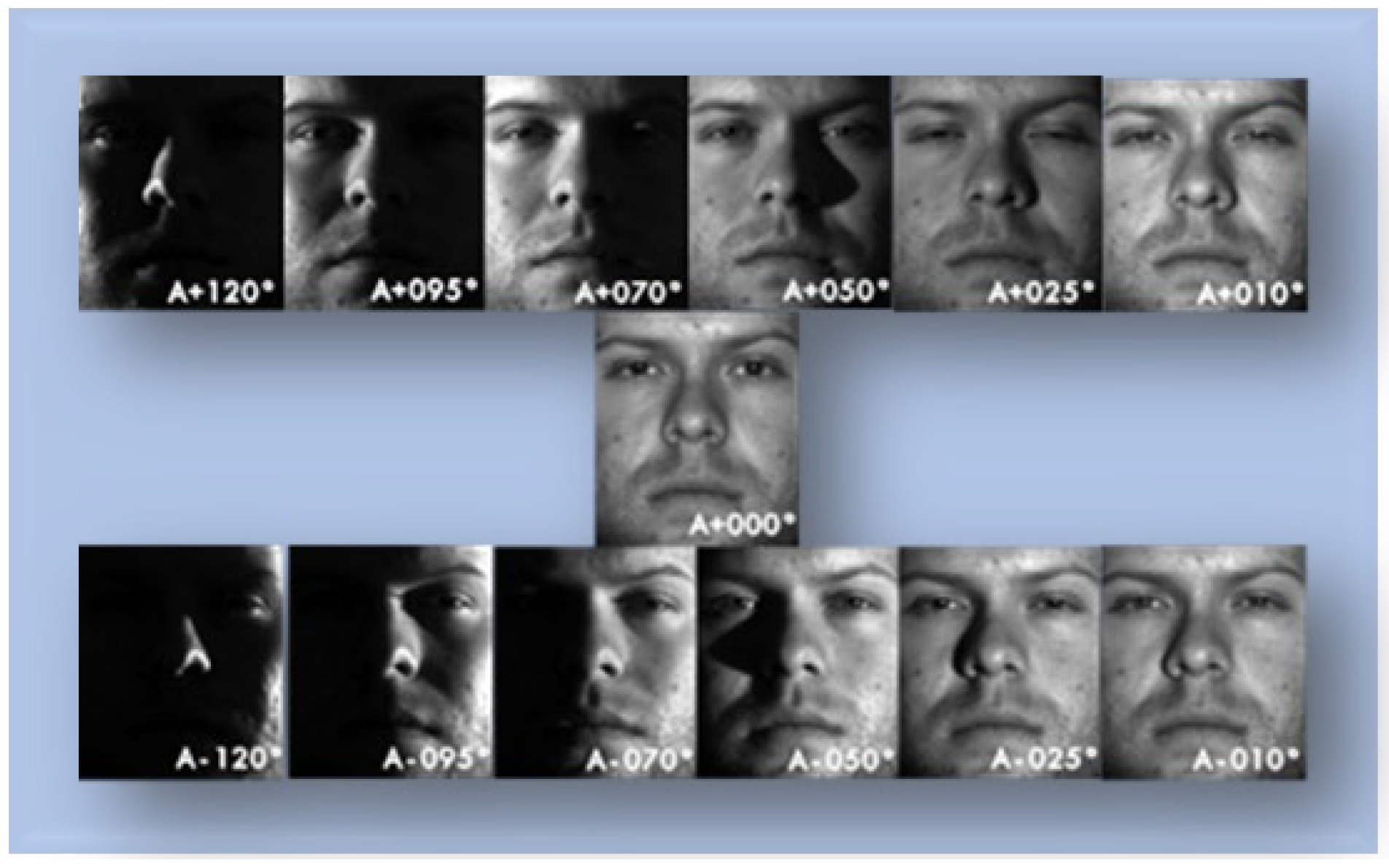
Table 3. List of images grouped in one of 7-groups (group-A+120--120E+00).
Group NameImage Name
A+120--120E+00yaleB01_P00A+000E+00
yaleB01_P00A+010E+00
yaleB01_P00A+025E+00
yaleB01_P00A+050E+00
yaleB01_P00A+070E+00
yaleB01_P00A+095E+00
yaleB01_P00A+120E+00
yaleB01_P00A-010E+00
yaleB01_P00A-025E+00
yaleB01_P00A-050E+00
yaleB01_P00A-070E+00
yaleB01_P00A-095E+00
yaleB01_P00A-120E+00
Table 4. Number of images in training set and test set after data enhancement.
ItemNumber of SheetsNumber of Images
Training set31 people × 62 sheets × 20 sheets × 0.830,752
Test set31 people × 62 sheets × 20 sheets × 0.27688
Total31 people × 62 sheets × 20 sheets38,440
Disclaimer/Publisher’s Note: The statements, opinions and data contained in all publications are solely those of the individual author(s) and contributor(s) and not of MDPI and/or the editor(s). MDPI and/or the editor(s) disclaim responsibility for any injury to people or property resulting from any ideas, methods, instructions or products referred to in the content.

