
Research on Modulation Signal Recognition Based on CLDNN Network


Abstract
:1. Introduction
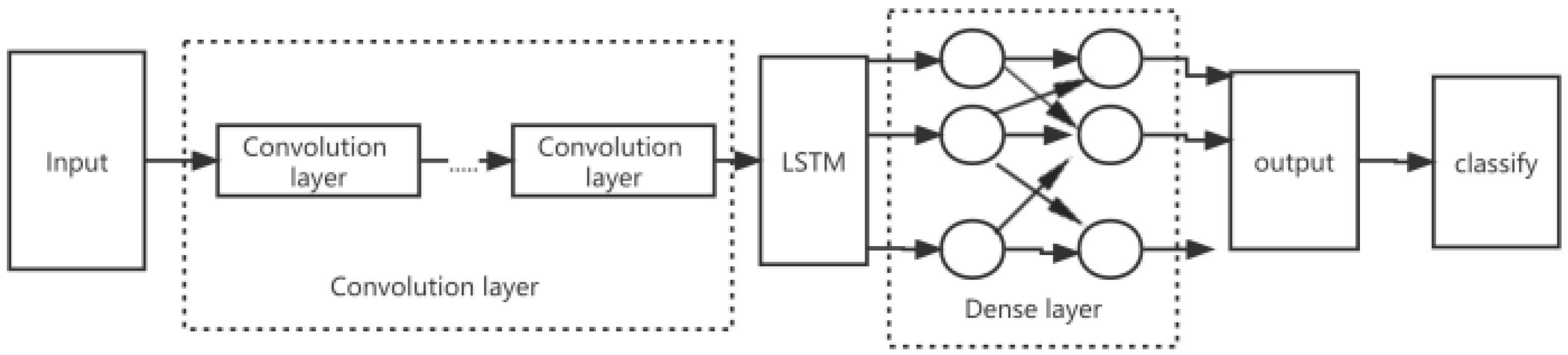
2. CLDNN Model
3. ASCLDNN Model
3.1. The CLDNN Network Model for Adaptive Modulation Signal Recognition Is Established
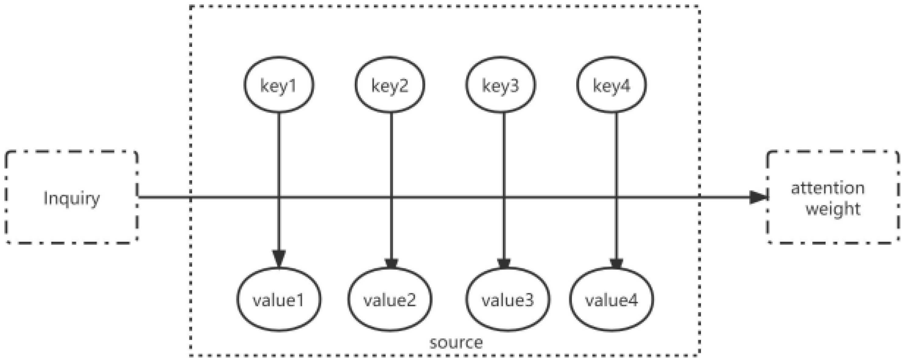
3.2. Attention Mechanism
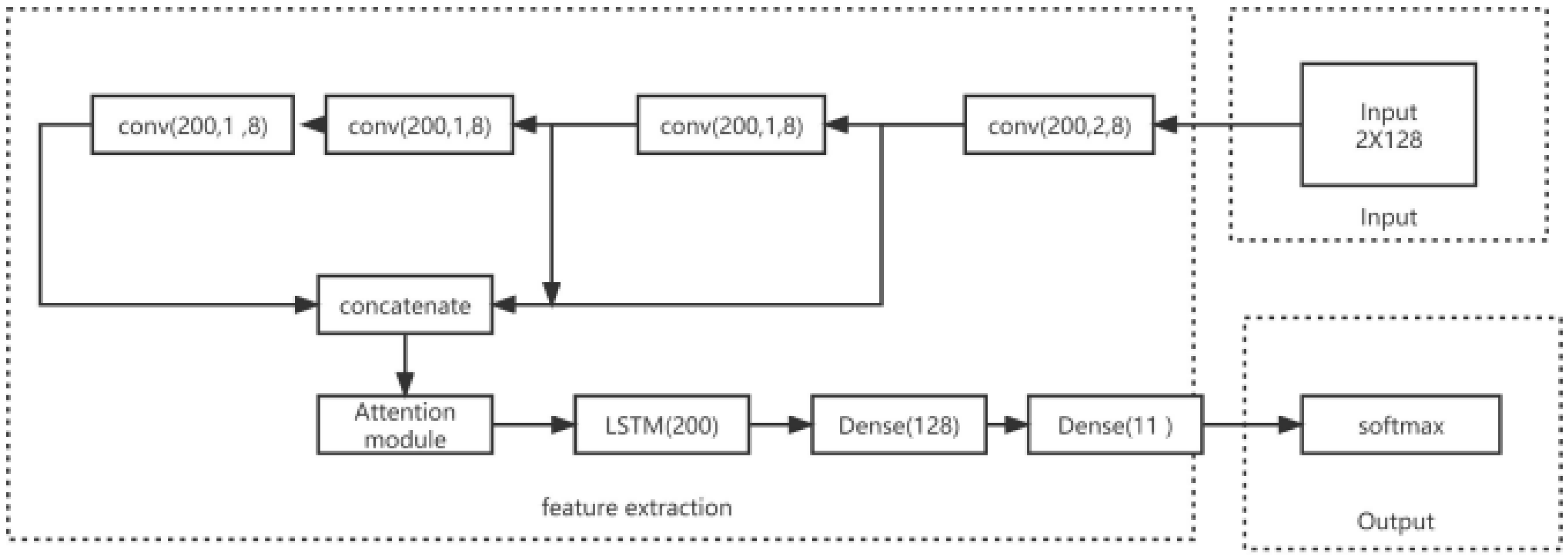
3.3. ASCLDNN Structure
3.4. Dataset
4. Experimental Results and Model Parameter Optimization
4.1. Influence of Attention Mechanism on Network Classification Ability
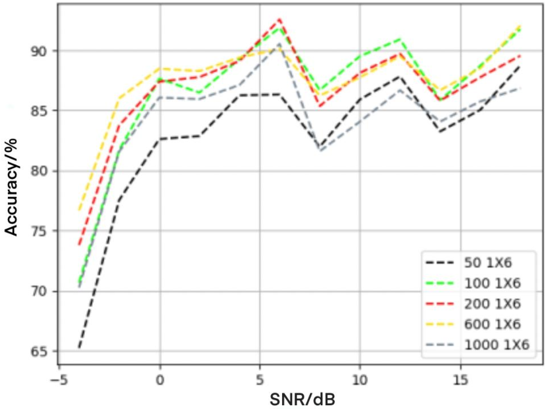
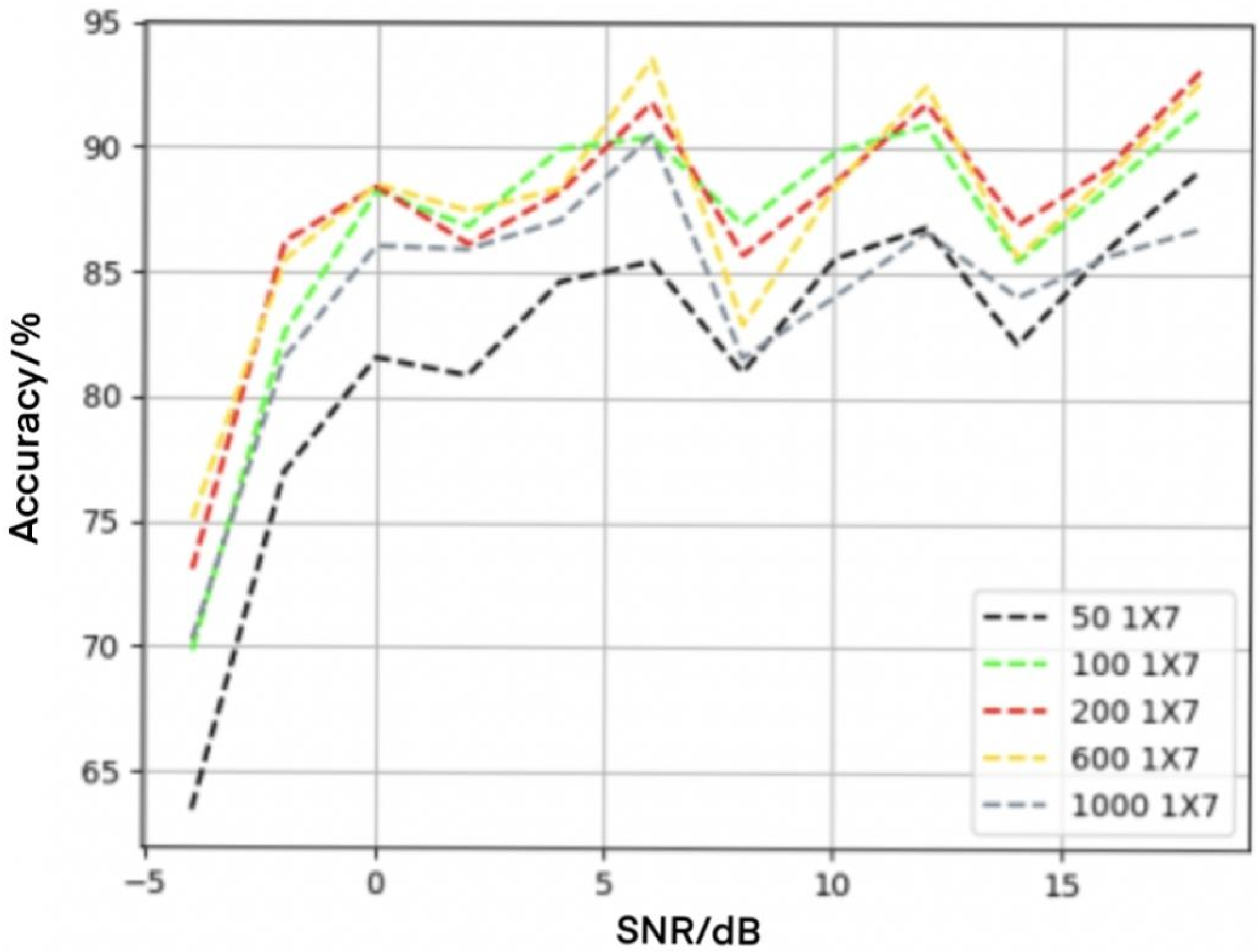
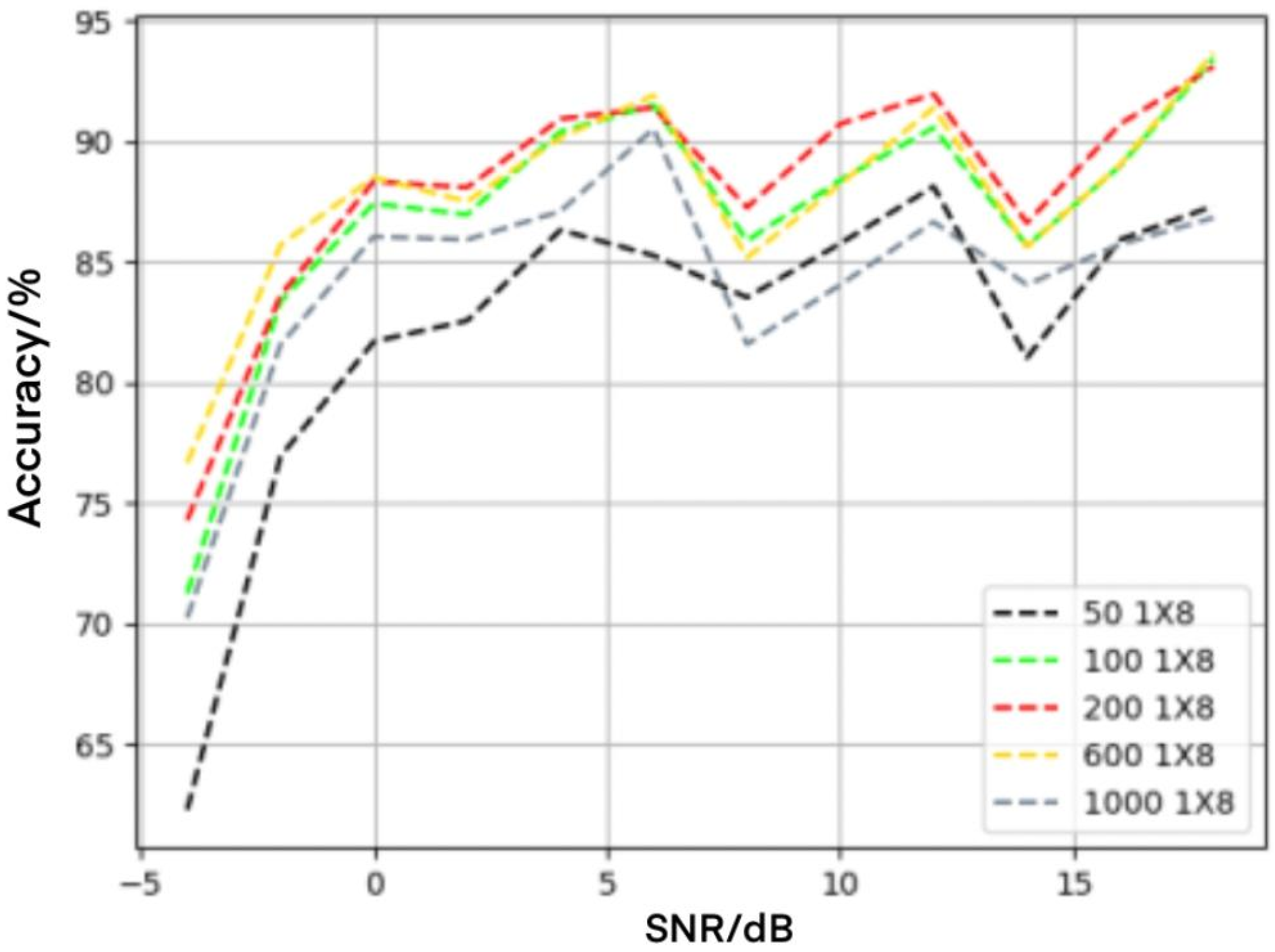
4.2. Influence of Convolution Check on Recognition Performance
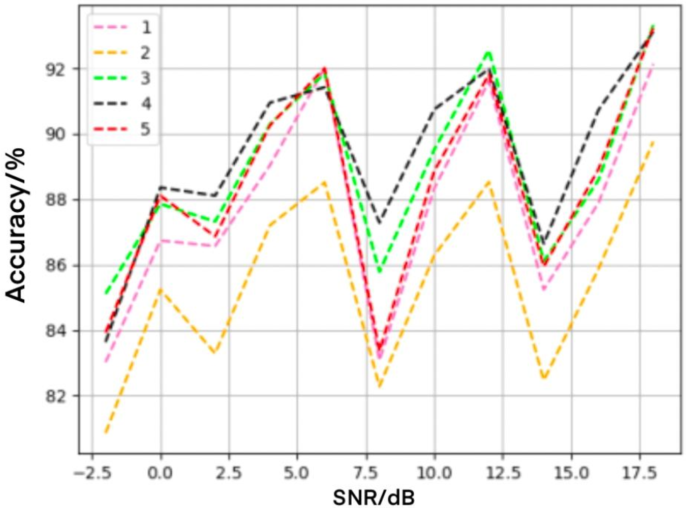
4.3. Influence of Convolution Layers on Recognition Performance
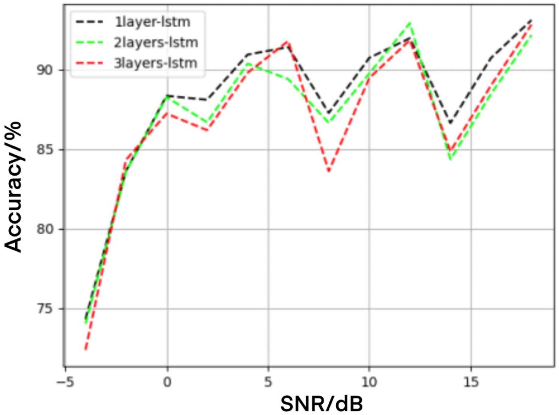
4.4. Influence of LSTM Layers on Recognition Performance
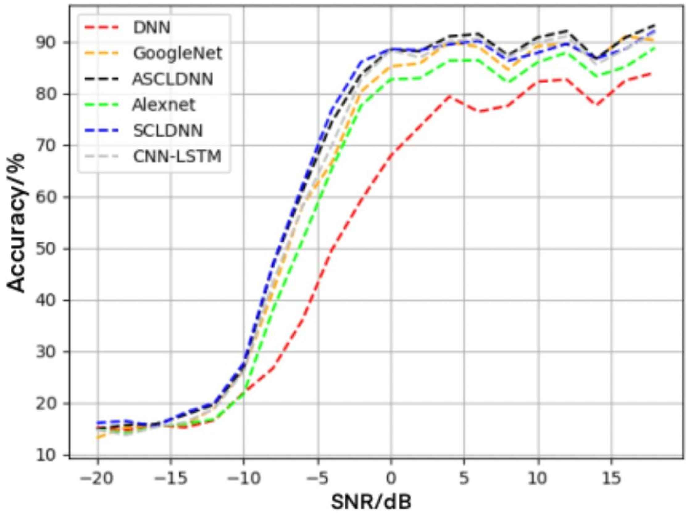
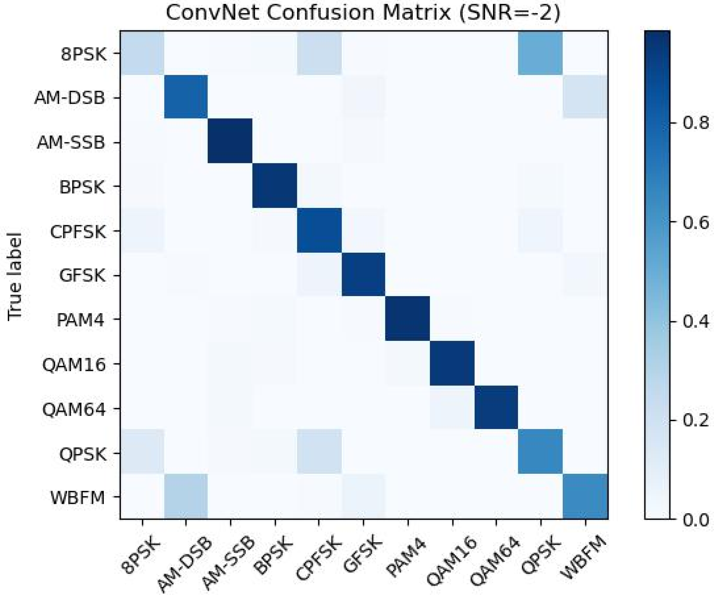
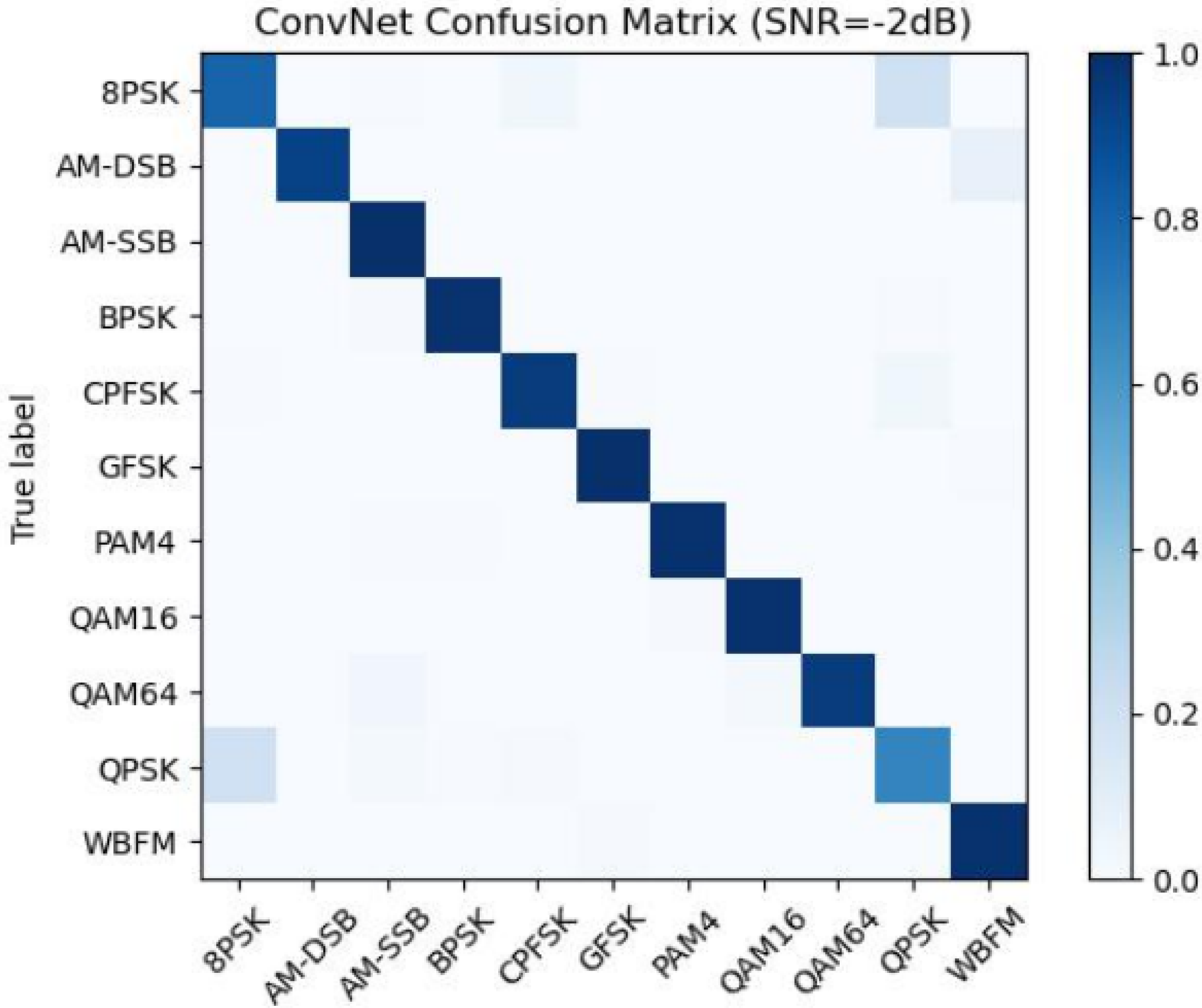
4.5. Performance Analysis of Different Networks
5. Conclusions
Author Contributions
Funding
Conflicts of Interest
References
- Object Management Group. Data Distribution Service for Real-Time Systems Specification Version 1.0. (2004-12). Available online: http://www.omg.org/spec/DDS/1.0 (accessed on 21 November 2019).
- Object Management Group. Data Distribution Service for Real-Time Systems Specification Version 1.1. (2005-12). Available online: http://www.omg.org/spec/DDS/1.1 (accessed on 21 November 2019).
- O’Shea, T.J.; Corgan, J.; Clancy, T.C. Convolutional radio mod-ulation recognition networks. In Proceedings of the International Conference on Engineering Applications of Neural Networks, Aberdeen, UK, 2–5 September 2016; Springer: Berlin/Heidelberg, Germany, 2016. [Google Scholar]
- West, N.E.; O’Shea, T.J. Deep architectures for modulation recognition. arXiv 2017, arXiv:1703. 09197. [Google Scholar]
- O’Shea, T.J.; Roy, T.; Clancy, T.C. Over the air deep learning based radio signal classification. arXiv 2017, arXiv:1712.04578. [Google Scholar] [CrossRef] [Green Version]
- O’Shea, T.; West, N. Radio machine learning dataset generation with gnu radio. In Proceedings of the GNU Radio Conference, Boulder, CO, USA, 12–16 September 2016. [Google Scholar]
- Zhang, M.; Zeng, Y.; Han, Z.; Gong, Y. Automatic modulation recognition using deep learning architectures. In Proceedings of the 2018 IEEE 19th International Workshop on Signal Processing Advances in Wireless Communications, Kalamata, Greece, 25–28 June 2018; pp. 281–285. [Google Scholar]
- Putra, H.A.; Kim, D.S. Node discovery scheme of DDS for combat management system. Comput. Stand. Author One Interfaces 2015, 37, 20–28. [Google Scholar] [CrossRef]
- Du, Y.; He, R. Electromagnetic radiation source identification technology based on deep learnin. Commun. World 2020, 27, 75–76. [Google Scholar]
- Sun, Y.; Tian, R.; Wang, X. Emitter signal based on improved cldnn Identification. Syst. Eng. Electron. Technol. 2021, 43, 42–47. [Google Scholar]
- Sainath, T.; Weiss, R.J.; Wilson, K.; Senior, A.W.; Vinyals, O. Learning the speech front end with raw waveform CLDNNs. In Proceedings of the Conference of the International Speech Communication Association, Dresden, Germany, 6–10 September 2015. [Google Scholar]
- Sainath, T.N.; Peddinti, V.; Kingsbury, B.; Fousek, P.; Nahamoo, D.; Ramabhadhran, B. Deep Scattering Spectra withDeep Neural Networks for LVCSR Tasks. In Proceedings of the Fifteenth Annual Conference of the International Speech Communication Association, Singapore, 14–18 September 2014. [Google Scholar]
- Hou, T.; Zheng, Y. Communication signal modulation recognition based on deep learning. Radio Eng. 2019, 49, 796–800. [Google Scholar]
- Li, J.; Jin, K.; Zhou, D.; Kubota, N.; Ju, Z. Attention mechanismr-based CNN for facial expression recognition. Neurocomputing 2020, 411, 340–350. [Google Scholar] [CrossRef]
- Zhang, W.; Liu, C. Application of convolutional neural network algorithm in speech recognition. Inf. Technol. 2018, 42, 147–152. [Google Scholar]
- Sainath, T.N.; Kingsbury, B.; Saon, G.; Soltau, H.; Mohamed, A.R.; Dahl, G.; Ramabhadran, B. Deep convolutional neural networks for large-scale speech tasks. Neural Netw. 2015, 64, 39–48. [Google Scholar] [CrossRef] [PubMed]
- Gao, L.; Wang, X.; Song, J.; Liu, Y. Fused GRU with semantictemporal attention for video captioning. Neuro- Comput. 2020, 395, 222–228. [Google Scholar]
- Xu, H.; Chai, L.; Luo, Z.; Li, S. Stock movement predictive network via incorporative attention mechanisms based ontweet and historical prices. Neurocomputing 2020, 418, 326–339. [Google Scholar] [CrossRef]
- Lei, Y.; Du, W.; Hu, Q. Face sketchrto-photo transfor- Automation with multi-scale self-attention Gan. J. Gate. Neuroinputing 2020, 396, 13–23. [Google Scholar]
- Chui, B.; Tian, R. Radar emitter recognition based on attention mechanism and improved cldnn. Syst. Eng. Electron. 2021, 43, 1224–1231. [Google Scholar]
- Sainath, T.N.; Vinyals, O.; Senior, A.; Sak, H. Convolutional, Long short-term memory, fully connected deep neural networks. In Proceedings of the 2015 IEEE International Conference on Acoustics, Speech and Signal Processing (ICASSP), South Brisbane, Australia, 19–24 April 2015. [Google Scholar]
- O’Shea, T.J. Available online: https://www.Deepsig.io/datasets (accessed on 8 January 2022).


| Model | Training Time (s) | Loss % | Training Accuracy % |
|---|---|---|---|
| SCLDNN | 0:11:22 | 0.405 | 60.7 |
| ASCLDNN | 0:3:34 | 0.329 | 64.2 |
| LSTM Layers | 1 | 2 | 3 |
|---|---|---|---|
| Average recognition rate of high signal-to-noise ratio | 89.93 | 88.91 | 88.66 |
| Highest recognition rate | 93.12 | 92.92 | 92.83 |
| Model | Training Time (s) | Number of Training Rounds | Loss % | Training Accuracy % |
|---|---|---|---|---|
| ASCLDNN | 0:3:34 | 17 | 32.9 | 64.2 |
| SCLDNN | 0:11:22 | 26 | 40.5 | 61.7 |
| GOOGLENET | 0:16:09 | 25 | 34.3 | 60.8 |
| ALEXNET | 0:05:39 | 5 | 26.1 | 58.9 |
| DNN | 0:7:41 | 40 | 12.9 | 54.6 |
| CNN-LSTM | 0:11:09 | 34 | 33.8 | 60.2 |
Publisher’s Note: MDPI stays neutral with regard to jurisdictional claims in published maps and institutional affiliations. |
© 2022 by the authors. Licensee MDPI, Basel, Switzerland. This article is an open access article distributed under the terms and conditions of the Creative Commons Attribution (CC BY) license (https://creativecommons.org/licenses/by/4.0/).
Share and Cite
Zou, B.; Zeng, X.; Wang, F. Research on Modulation Signal Recognition Based on CLDNN Network. Electronics 2022, 11, 1379. https://doi.org/10.3390/electronics11091379
Zou B, Zeng X, Wang F. Research on Modulation Signal Recognition Based on CLDNN Network. Electronics. 2022; 11(9):1379. https://doi.org/10.3390/electronics11091379
Chicago/Turabian StyleZou, Binghang, Xiaodong Zeng, and Faquan Wang. 2022. "Research on Modulation Signal Recognition Based on CLDNN Network" Electronics 11, no. 9: 1379. https://doi.org/10.3390/electronics11091379